Engenharia Agrícola
ISSN: 1809-4430 (on-line) www.engenhariaagricola.org.br
1 Universidade Federal de Viçosa/ Viçosa - MG, Brasil.
3 Universidade Federal de Minas Gerais/ Belo Horizonte - MG, Brasil.
Received in: 1-19-2018 Accepted in: 6-22-2018
Doi: http://dx.doi.org/10.1590/1809-4430-Eng.Agric.v38n5p751-759/2018
ESTIMATION ON THE CONCENTRATION OF SUSPENDED SOLIDS FROM TURBIDITY IN
THE WATER OF TWO SUB-BASINS IN THE DOCE RIVER BASIN
Amanda R. M. de Oliveira
1, Alisson C. Borges
2*, Antonio T. Matos
3, Moysés Nascimento
12*Corresponding author.Universidade Federal de Viçosa/ Viçosa - MG, Brasil. E-mail: borges@ufv.br
KEYWORDS
adjusted boxplot,
water quality
monitoring, variables
dummy.
ABSTRACT
Knowing the relationship between the total suspended solids concentration (TSS),
turbidity in the waters, and that turbidity analysis can be done faster and in less expensive
way, this study aimed to obtain mathematical model to estimate the total suspended solids
(TSS) concentration from the turbidity values for waters of Doce river basin. For this
purpose, it was used the water quality database of the Minas Gerais Institute of Water
Management (IGAM). The data were pre-treated using the adjusted boxplot technique
followed by adjustment of curves for the different management units and rainfall regime
period. It was verified the possibility of a single curve through the dummy variable
technique, subsequently. With the results it was observed that the adjusted boxplot
technique proved to be useful for environmental data. Linear relationships with R² values,
as a rule, were higher than 0.6, however, it was not possible to develop a single model. It
is concluded that the generated models presented good adjustments being able to be used
for predicting the concentration of TSS as a function of turbidity. However, each
management unit in each period of rainfall regime presents particularities that were
reflected in the prediction models.
INTRODUCTION
Water does not appear in the environment in the
purely molecular form (H2O), due to its solvent properties
and its ability to transport particles. In it, compounds of natural and anthropogenic origin are present (von Sperling, 2014), such as salts, metals, microorganisms, organic matter, among others. These constituents are responsible for their characterization (von Sperling, 2014) and, therefore, for their classification according to the nobility of their use.
In this sense, an important parameter for the analysis of water quality is the concentration of total suspended solids (TSS) because these types of solids are good indicators of physical and esthetic degradation of surface water quality, being also good indicators of the presence of other pollutants (Hannouche et al., 2011; Kusari & Ahmedi, 2013; Rügner, et al., 2013).
The reduction in photosynthetic activity due to the impediment of the passage of sunlight, the transport of pollutants such as phosphorus, mercury and hydrophobic organic compounds are associated with TSS high concentrations in the water (Rügner et al., 2013).
TSS can also cause depletion on dissolved oxygen (DO) due to the increase in surface water temperature caused by higher absorption of solar energy by such solids (Naveedullah et al., 2016). Large amounts of suspended solids (SS) can affect procreation of fish and invertebrates due to obstruction on breeding habitat (Naveedullah et al., 2016). In addition, TSS can serve as a shelter for pathogenic microorganisms and may be associated to bacterial contamination (Bakan et al., 2010; Henning et al., 2014).
Following this line of reasoning, another parameter that can give indicative of TSS concentration is the turbidity which is easy to measure, that because the main responsible factor for turbidity is the SS (Hannouche et al., 2011).
The turbidity is quantified by the nephelometric method which is based on the comparison of the light intensity spread over by the sample under defined conditions, with the light intensity spread by suspension considered standard. So, as great the intensity of the spread light is greater is the turbidity in the sample under analysis (APHA et al., 2017). The used equipment for the reading is the turbidimeter which consists of a nephelometer, being the turbidity expressed in nephelometric turbidity units
(NTU). In in situ monitoring probes, the sensor consists of
an infrared nephelometric turbidimeter.
There have been previous attempts to use the turbidity measure to estimate the TSS concentration (e.g. Suk et al., (1998), Hannouche et al. (2011) and Kusari & Ahmedi (2013)), but there is no universal relation between turbidity and TSS. It is necessary the development of specific relations in each place (Kusari & Ahmedi, 2013).
Knowing the existence of direct relationship between the concentration of suspended solids present in the water and its turbidity, and that the analysis of the turbidity is processed faster and at lower cost, this study had the objective of obtaining models to estimate the
concentration of TSS by means of the turbidity data in waters of two important sub-basins of Doce river, being those from Piranga and Piracicaba river.
MATERIAL AND METHODS
Study area
The watershed of the Doce River is located in the
Southeast region, between the parallels 17° 45’ and 21°15’
S and the meridians 39°30’ and 43°45’ W, dividing
between the states of Minas Gerais (86% of the drainage area) and Espírito Santo (Ecoplan Lume Consortium, 2010). With a population of more than 3.5 million inhabitants, covering 230 municipalities and a drainage area of approximately 86,715 km², this basin is part of the Southeast Atlantic hydrographic region (Ecoplan Lume Consortium, 2010).
Its springs are located in the state of Minas Gerais, in the mountains of Mantiqueira and Espinhaço. Their waters are drained to the town of Regencia, in the state of Espírito Santo, where they flow into the Atlantic Ocean (Figure 1). In this basin there are two rivers of federal dominance, being they the Doce river and the Jose Pedro river, affluent of the Manhuaçu river (Ecoplan Lume Consortium, 2010).
Adapted from Ecoplan Lume Consortium (2010)
FIGURE 1.Map of the river basin of the Doce river.
The Doce river basin was chosen because of its great socioeconomic and political importance, and because it is a basin with intense economic activity and population occupation.
In the State of Minas Gerais, the Doce river basin is divided into six Water Resources Planning and Management Units (WRPMUs): Piranga River Basin Committee (DO1); Piracicaba River Basin Committee (DO2); Santo Antônio River Basin Committee (DO3); Hydrographic Basin Committee of the Suaçuí River
(DO4); Caratinga River Basin Committee (DO5); and the Manhuaçu River Basin Committee (DO6) (Ecoplan Lume Consortium, 2010).
Characteristics of the data
In order to obtain models for estimating TSS concentration from the turbidity data, a survey was made
on the water surface quality database available at “Portal
InfoHidro” by the Instituto Mineiro de Gestão das Águas
(IGAM) which monitors the quality of surface and groundwater in Minas Gerais since 1997 - known as the
“Águas de Minas Project” - generating data that are
indispensable for the correct management of water resources.
Currently, IGAM has in its qualitative monitoring network sixty-four (64) sampling stations located in the Doce river basin; 15 of these stations are located at WRPMU in Piranga river, and 13 in the WRPMU in Piracicaba river, that is, 44% of the stations basin are in these important WRPMUs.
In order to evaluate the water quality, 56 water quality parameters are analyzed among them are the turbidity and the concentration of TSS. The collections of samples and the respective analyzes are carried out by the National Service of Industrial Learning - Technological Center Unit of Minas Gerais (SENAI - CETEC).
The frequency of the review varied between semiannual, quarterly, every three months and monthly. In all, there were 3062 collections in the entire Doce river basin between 1997 and 2014. Of these collections, 793 were made at the WRPMU in Piranga river, and 688 at the WRPMU in Piracicaba river (48% of the total).
Pre-processing of data
Usually environmental data present censored, lost values, as well as outliers (Sabino et al., 2014). To avoid any problems that these types of values may cause in statistical analyzes, the database must be handled.
Thus, in this study, the methodology presented by Sabino et al. (2014) was used to treat the censored values. According to this methodology, values below the minimum detection limit are replaced by half the minimum detection limit; yet the values that are above the maximum measured value are maintained by the responsible organ.
In the case of missing data, the sample that did not present one of the two studied parameters or did not present any of the two parameters, was excluded, since, in this study, a relation between TSS and turbidity was sought if one of the parameters (or both parameters) is not measured, there is not a pair to account in the regression models to be adjusted.
For the investigation and later elimination of the outliers, we used the adjusted boxplot method, proposed by Vandervieren & Hubert (2004).
Statistical analyzes
After the data pre-treatment, linear regression models were adjusted for the two WRPMUs: Piranga and Piracicaba. In the adjusted models, the pluviometric regime of the units was considered, that is, simple linear regression models were adjusted for the rainy season - which, according to the Ecoplan Lume Consortium (2010), extends from October to March, when rain volumes vary
from 800 to 1300 mm - and for the dry period - which extends from April to September, when rain volumes vary from 150 to 250 mm (Ecoplan Lume Consortium, 2010).
With the models properly adjusted, we sought to verify the equality of the full / dry regression models and Piranga / Piracicaba. That is, evaluate between the equations if the estimated parameters are statistically the same, in order to obtain a single equation. According to Regazzi & Silva (2010), this is a very frequent practice in regression analysis. For this, it was used the dummy variables method.
The dummy variable method along with the identity model method are the most relevant for comparisons between linear regression equations (Magalhães & Andrade, 2009). The methods present very similar results however, with the dummy variables there is lower probability of occurrence on Type I Error (rejecting the null hypothesis, being it true) and Type II Error (not rejecting the null hypothesis, being it false) (Magalhães & Andrade, 2009) that is why in this study we chose to use it. This method consists in the inclusion of additive and
multiplicative binary variables, the dummy variables,
which assume values 0 and 1. Then, new models, including these variables, are adjusted and their
coefficients are tested (Student’s t-test) (Magalhães &
Andrade, 2009).
RESULTS AND DISCUSSION
Pre-processing of data
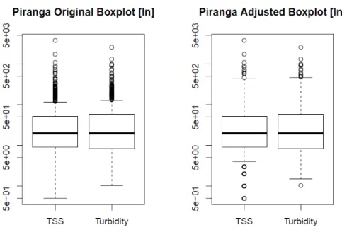
Initially, the boxplot method was used (here it will be called the original boxplot); however, it was observed that a large number of values were classified as being discrepant (approximately 15% of the values); which, if removed from analyzes could compromise the veracity of the results.
The original boxplot method, that it is the “Tukey
fences” (Lyra, 2014), it assumes that the data follow a
normal distribution. Performing tests of adherence to normal and lognormal distributions - Anderson-Darling,
Kolmogorov-Smirnov, Shapiro-Wilk and Ryan-Joiner – it
was observed that there was no adherence to the
distribution curves analyzed (p-value ≤ 0.05) in the data of
none of WRPMUs. Vandervieren & Hubert (2004) explain that, when conventional methods are used in the analysis of distorted data (abnormals), many points are usually classified as outliers because the cut-off values are derived from the normal distribution.
TSS – Total suspended solids
Note: The representation of data in the form of natural logarithm was made for better limits visualization.
FIGURE 2.Comparison between adjusted boxplot and original boxplot method to investigate the existence of outliers on TSS
values and turbidity for the Piranga River WRPMU.
Using the adjusted boxplot, the amount of values held in the distribution is greater (approximately, 8% of the data were censored).
After the elimination of the missing values and subsequent elimination of the outliers from 793 performed collections at the WRPMU in the Piranga river, 730 remained, being 396 data from the rainy period and 334 from the dry period; and out of 688 collections made at the WRPMU in the Piracicaba river, 613 remained, being 302 data from the rainy period and 311 from the dry period. This means that, for the statistical analysis, we still have approximately 88% of the total initial collections.
Adjustment of regression models
Proceeding to the analysis of variance (ANOVA), considering the simple linear regression model, we can observe that the turbidity has a significant linear
relationship with the TSS concentration, in all adjusted
models (p-value ≤ 0.01). Other authors, also studying the
relationship between these two parameters in stream water, have found linear relationship between them (e.g. Suk et al., 1998), Daphne et al. (2011); Rügner et al. (2013)). Pavanelli & Bigi (2005), using samples prepared in laboratory with specific solids concentrations, also found linear relationship between these variables. Already Bhargava & Mariam (1990) observed both a linear and curvilinear relationship; however, these authors studied the relationship between turbidity and TSS content in suspensions in 4 different types of soils. The difference between the ratios for each type of soil suspension is mainly due to variations in the spectral characteristics of each studied material (Bhargava & Mariam, 1990).
Tables 1 and 2 show the regression coefficient estimates for the rainy and dry periods of the two WRPMUs, Piranga and Piracicaba.
TABLE 1. Regression coefficients of the simple linear model for TSS concentration as a function of turbidity at the Piranga WRPMU for the rainy and dry periods.
Factors Regression coefficient Standard deviation Estat. t p- value
Rainy Turbidity Intercept 9.99 0.86 2.47 0.02 30.71 4.04 <0.001 <0.001
Dry Turbidity Intercept 4.36 0.79 0.88 0.02 46.20 4.98 <0.001 <0.001
TABLE 2. Regression coefficients on simple linear model for TSS concentration as a function of the turbidity at the Piracicaba WRPMU for the rainy and dry periods.
Factors Regression coefficient Standard deviation Estat. t p-value
Rainy Turbidity Intercept 10.18 0.64 2.27 0.03 25.26 4.49 <0.001 <0.001
The adjustment coefficients were significant
(p-value ≤ 0.01) for all adjusted models (Tables 1 and 2). It is
also noted that, in the analysis interval, increase in turbidity reflects an increase in the concentration of TSS, fact also evidenced by the authors above mentioned.
According to Rügner et al. (2013), angular coefficients between 1 and 2 have been reported in the literature, but these authors present other studies that obtained angular coefficients from 0.75 to 3.3. Suk et al. (1998), monitoring the concentration of TSS and turbidity in a river in 25 different time periods, observed angular coefficients between 0.2 and 2.8. Then, the coefficients obtained in the present study are within the ranges found in the literature.
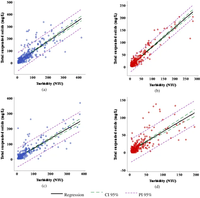
It was found in some samples that, although the turbidity value was high, the value of the TSS concentration was low, as can be observed in the graphs of Figure 3. This fact can be consequence of a high concentration in colloidal solids (muddy water) in the collected samples. These solids can be counted in the turbidity at some point of water turbulence; however, they
are not considered in TSS concentration, once they must
present size range from 100μm to103μm (von Sperling,
2014), and the colloidal solids are in the range of 10-3μm to
100μm (von Sperling, 2014).
It is also observed the opposite, that is, in some samples, although the value of turbidity is low, the value of the TSS concentration is high. According to Metcalf & Eddy et al. (2014), turbidity measurement, especially low values, presents high degree of variability depending on the light source and the measurement method which could explain what happened with these samples. Daphne et al. (2011) also verified the possibility of low turbidity values related to concentration of TSS in the sample of a river, and that this may be due to a fraction of fine sand present in the samples that was quickly installed below the monitored zone by the turbidimeter. This fact was found by observing such fraction of sand trapped in a set with
other suspended solids during filtration using a 0.6 μm
glass fiber filter when measuring TSS concentration (Daphne et al., 2011).
(a) (b)
(c) (d)
Regression CI 95% PI 95%
Note: CI - Confidence Interval and PI - Prediction Interval
FIGURE 3.Turbidity dispersion graphs in water samples collected at the WRPMU in the Piranga river during the rainy (a) and
In both cases, the reason for this disproportion between turbidity and TSS may also be the fact that turbidity is measured by an optical property, subject to the interference of shape, size, refractive index and particle density, as well as color of the water, but little influence on the concentration of the suspended material (Bhargava & Mariam, 1990; Gippel, 1995; Daphne et al., 2011; Hannouche et al., 2011; Rügner et al., 2013). In other words, the relationship between TSS and turbidity is dependent on the variations in the spectral characteristics of the suspended material (Daphne et al., 2011).
Reading and/or analyzing errors may also have provided the above problems. Gippel (1995) shows that turbidity data measured in laboratories can be censored because of particle agglomeration problems in the sample conditioning vessel. Yet, Suk et al. (1998) report that, for in situ monitoring, the compromise of the collected data may occur due to the high biological growth rates in the instruments. Pavanelli & Bigi (2005) demonstrated that by storing the samples for a long period (1 month) - at room temperature, exposed to daylight - there is an increase in water turbidity due to the development of microorganisms and algae, aggregation of clays and flocculation, in addition to other biological reactions and gas production.
Following the evaluation of the adjusted models we verified possible deviations of the assumptions model, consequently, the adjustment of the same, investigating if the residues present normal distribution. For both WRPMUs, in the rainy and dry periods, there was no
adherence to the normal distribution curve (p-value ≤ 0.05)
in none of the tests - Anderson-Darling, Shapiro-Wilk, Kolmogorov-Smirnov, Ryan-Joiner. According to Minitab (2014), p-value accuracy is sensitive to non-normal residual errors when dealing with small samples (less than 15). Therefore, because the samples are sufficiently large, the adjustment of the models is not compromised by the non-normality of the residues.
Finally, the coefficient of determination value (R²) for the rainy and dry periods in the Piranga river was respectively, 0.71 and 0.87. For the WRPMU in the Piracicaba river in the rainy season R² was 0.68, and for the dry period, 0.54. It should be noted that R² values are high - except for the dry period of the Piracicaba river unit - then there are indications that the simple linear model adjusted well to the data set analyzed for the rainy and dry periods of the two WRPMUs, Piranga and Piracicaba. However, for Barros Neto et al. (2007), models with R² <0.60 should be used only as trend indicators, never for predictive purposes. Therefore, only the adjusted model for the dry period at the Piracicaba WRPMU cannot be used to predict the concentration of TSS.
Rügner et al. (2013) present R² values in the literature varying from 0.73 to 0.99; however, these authors, studying the relationship between TSS and turbidity in basins in Southeastern Germany, found R² ranging from 0.59 to 0.98. It can be said, then, that the values of determination coefficients obtained in this study are comparable to those in the literature. Recalling that several factors influence the relation between TSS and turbidity - as earlier commented - then we cannot establish a criterion in this regard.
The low value of R² in the dry period at the Piracicaba WRPMU is due to the fact previously described: many points with high turbidity value and low value on TSS concentration and also many points with low value of turbidity and high concentration of TSS. When these values were withdrawn, a better adjustment of the model was observed, which can be noticed by increasing the R² value to 0.78.
Suk et al. (1998) observed that the low concentrations of TSS disrupted the good adjustment of the models. Daphne et al. (2011) found that, as the TSS increases, the turbidity uncertainty is also increased with higher consistency of a maximum TSS concentration on
approximately 50 mg L-1 - obtaining R² at 0.81, by
restricting the range of TSS concentration. As shown above, when we extracted the values that compromised the good adjustment of the model, we obtained R² value close to that obtained by Daphne et al. (2011), but the maximum concentration of TSS that allowed a greater consistency in
the results was approximately 90 mg L-1.
Even as trend indicators, the models would be of great value. As already mentioned, monitoring the water quality is very important, but it is not an easy practice (Goher et al., 2014). Having models that indicate trend of the magnitude on certain parameter, if there are any discrepant value models that indicate trend of the magnitude of a given parameter are observed, if some discrepant value is observed, more accurate analyzes can be carried out and then measures can be taken (Kusari & Ahmedi, 2013). This would contribute to a more practical and economically viable process for monitoring water quality, especially in developing countries (Kusari & Ahmedi, 2013, Rügner et al., 2013).
Verification of model equality for prediction of TSS concentration
Tables 3 and 4 show the obtained results using the dummy variables method for rainy and dry periods - assigning D = 0 for the dry period and D = 1 for the rainy period.
TABLE 3. Estimation of the regression coefficients on new adjusted model for TSS concentration in collected water samples at Piranga WRPMU.
Factors Estimate Standard error Estat. t p-value
Intercept 4.36 1.94 2.24 0.03 *
D 5.64 2.73 2.07 0.04 *
Turbidity 0.79 0.04 20.8 <0.001 ***
D: Turbidity 0.07 0.04 1.63 0.10 ns
Note: * significant at 0.05 probability level; ** significant at 0.01 probability level; *** significant at 0.001 level of probability; ns not
TABLE 4. Regression coefficients on new adjusted model for TSS concentration in water samples collected at the Piracicaba WRPMU.
Factors Estimate Standard error Estat. t p-value
Intercept 4.58 1.83 2.50 0.01 *
D 5.60 2.57 2.17 0.03 *
Turbidity 0.56 0.04 12.6 <0.001 ***
D: Turbidity 0.08 0.05 1.63 0.10 ns
Note: * significant at 0.05 probability level; ** significant at 0.01 probability level; *** significant at 0.001 level of probability; ns not
significant by Student’s t-test. D - dummy variable (D = 0, dry period; D = 1 rainy period).
For both WRPMUs the coefficient D is significant. Therefore, we can see sample evidence for the equality hypothesis of intercepts on the linear models for the two periods (rainy and dry) is not true. However, the interaction coefficient D: Turbidity is not significant in both WRPMUs. This means that there are indications for linear models on the two periods (rainy and dry) are parallel. That is, for both WRPMUs rainy and dry models present angular coefficients statistically equal; however, do not have equality on intercept.
The possibility of equality between WRPMU models for each period was also tested. For the Piranga WRPMU was assigned D = 1, and for the Piracicaba WRPMU was assigned D = 0. In the same way, new models of the whole dataset of each period were adjusted (Piranga and Piracicaba) and including as dummy variables. The obtained results using the dummy variables method are presented in Tables 5 and 6.
TABLE 5. The regression coefficients of the new adjusted model for the concentration of TSS in water samples collected from Doce river basin during the rainy period.
Factors Estimate Standard error Estat. t p-value
Intercept 10.2 2.54 4.01 <0.001 ***
D -0.18 3.43 -0.05 0.96 ns
Turbidity 0.64 0.03 22.5 <0.001 ***
D: Turbidity 0.22 0.04 5.65 <0.001 ***
Note: * significant at 0.05 probability level; ** significant at 0.01 probability level; *** significant at 0.001 level of probability; ns not
significant by Student’s t-test. D - dummy variable (D = 0, Piracicaba WRPMU; D = 1, Piranga WRPMU).
There are indications that Piranga WRPMU model and Piracicaba WRPMU model, for both periods of the year, are not parallel. However, there is evidence that the hypothesis of intercepts equality of on the linear models for two WRPMUs (Piranga and Piracicaba) is true. Thus, it can be said that the Piranga WRPMU and Piracicaba WRPMU models, in both periods of the year, have equal intercept, but are not parallel.
TABLE 6. The regression coefficients on new adjusted model for TSS concentration in water samples collected from the Doce river basin during the dry period.
Factors Estimate Standard error Estat. t p-value
Intercept 4.58 1.09 4.20 <0.001 ***
D -0.23 1.47 -0.15 0.88 ns
Turbidity 0.56 0.03 21.1 <0.001 ***
D: Turbidity 0.23 0.03 6.88 <0.001 ***
Note: * significant at 0.05 probability level; ** significant at 0.01 probability level; *** significant at 0.001 level of probability; ns not
significant by Student’s t-test. D - dummy variable (D = 0, Piracicaba WRPMU; D = 1, Piranga WRPMU).
The adjustment of a single model for the two WRPMUs under study, in order to contemplate the rainy and dry periods was not possible. These results corroborate with those by Hannouche et al. (2011) who verified variation between the models for drought and flood conditions and also between sites. These authors explain that in urban wastewater or rainwater the characteristics of suspended solids are heterogeneous and variable, so it is possible occur variations in time and space (Hannouche et al., 2011).
According to Daphne et al. (2011) the relation between TSS and turbidity depend on the variations in the spectral characteristics of the suspended material, so the relation is unique in each situation, as can be observed in the present study and also in the study by Hannouche et al.
(2011). It is necessary, then, to use one model for each situation.
In each situation, the equations describing the adjusted models to predict TSS concentration as a function of turbidity in the Piranga WRPMU during rainy and dry periods are presented in eqs (1) and (2), respectively:
TSSrainy = 0.86 Turbidity + 9.99 (1)
TSSdry = 0.79 Turbidity + 4.36 (2) Where:
TSSrainy – concentration on total suspended solids
for the rainy period (mg L-1);
TSSdry– concentration on total suspended solids for
the dry period (mg L-1),
The equations describing the adjusted models to predict the TSS concentration as a function of turbidity on the Piracicaba WRPMU in the rainy and dry periods are presented in eqs (3) and (4), respectively:
TSSrainy = 0.64 Turbidity + 10.18 (3)
TSSdry = 0.56 Turbidity + 4.58 (4)
Where:
TSSrainy – concentration on total suspended solids
for the rainy period (mg L-1);
TSSdry– concentration on total suspended solids for
the dry period (mg L-1),
Turbidity – turbidity measurement (NTU).
CONCLUSIONS
The generated models with the total suspended solids concentration and turbidity data presented good adjustments and could therefore be used to predict the concentration on total suspended solids as a function of turbidity. Except for the dry period model at the Piracicaba WRPMU.
Each basin, in each period of the year, presents its peculiarities that were reflected in the models to predict the concentration of total suspended solids as a function of turbidity. It was not possible, then, to adjust a single model for the two WRPMUs under study, in order to contemplate the rainy and dry periods, making necessary to use one model for each situation.
ACKNOWLEDGEMENTS
The authors express gratitude to CNPq and IGAM.
REFERENCES
APHA [American Public Health Association]; AWWA [American Water Works Association]; WEF [Water Environment Federation] (2017) Standard methods for the examination of water and wastewater. American Public Health Association (APHA): Washington, DC, USA, (23). Bakan G, Özkoç HB, Tülek S, Cüce H (2010) Integrated
environmental quality assessment of the Kızılırmak River
and its coastal environment. Turkish Journal of Fisheries
and Aquatic Sciences 10(4): 453–462.
Barros Neto B, Scarminio IS, Bruns RE (2007) Como Fazer Experimentos: Pesquisa e Desenvolvimento na Ciência e na Indústria. Campinas, Editora Unicamp, 3 ed. 401p.
Bhargava DS & Mariam DW (1990) Spectral reflectance relationships to turbidity generated by different clay materials. Photogrammetric Engineering and Remote
Sensing 56(2): 225–229.
CONSÓRCIO ECOPLAN LUME (2010) Plano integrado de recursos hídricos da bacia hidrográfica do Rio Doce e planos de ações para as unidades de planejamento e gestão de recursos hídricos no âmbito da bacia do Rio Doce. Governador Valadares, Consórcio Ecoplan-Lume, 1 ed. 478p.
Daphne LHX, Utomo HD, Kenneth LZH (2011)
Correlation between turbidity and total suspended solids in Singapore rivers. Journal of Water Sustainability 1(3):
313–322.
Gippel CJ (1995) Potential of turbidity monitoring for measuring the transport of suspended solids in streams.
Hydrological processes 9(1): 83–97.
Goher ME, Hassan AM, Abdel-Moniem IA, Fahmy AH, El-sayed SM (2014) Evaluation of surface water quality and heavy metal indices of Ismailia Canal, Nile River, Egypt. The Egyptian Journal of Aquatic Research 40(3):
225–233. DOI: https://doi.org/10.1016/j.ejar.2014.09.001
Hannouche A, Chebbo G, Ruban G, Tassin B, Lemaire BJ, Joannis C (2011) Relationship between turbidity and total suspended solids concentration within a combined sewer
system. Water Science and Technology 64(12): 2445–2452.
Henning E, Walter OMCF, Souza NS, Samohyl RW (2014) Um estudo para a aplicação de gráficos de controle estatístico de processo em indicadores de qualidade da
água potável. Sistemas & Gestão 9(1): 2–13.
Kusari L & Ahmedi F (2013) The use of Turbidity and Total Suspended Solids Correlation for the Surface Water Quality Monitoring. International Journal of Current
Engineering and Technology 3(4): 1311–1314.
Lyra TF (2014) Métodos para detecção de outliers em séries de preços do índice de preços ao consumidor. Dissertação (Mestrado), Fundação Getulio Vargas, Escola de Matemática Aplicada.
Magalhães SR & Andrade EA (2009) Teste para verificar a igualdade de modelos de regressão e uma aplicação na
área médica. e-xacta 2(1): 34–41.
Metcalf & Eddy, Burton FL, Stensel HD, Tchobanoglous G (2014). Wastewater engineering: treatment and resource recovery. New York, McGraw Hill, 5 ed. 1815p.
Minitab (2014) Simple regression. In: Minitab Assistant, 2014. Disponível em: https://support.minitab.com/en-us/minitab/18/Assistant_Simple_Regression.pdf. Acesso em: 6 jun. 2016.
Naveedullah N, Hashmi MZ, Yu C, Shen C, Muhammad N, Shen H, Chen Y (2016) Water Quality Characterization of the Siling Reservoir (Zhejiang, China) Using Water
Quality Index. CLEAN–Soil, Air, Water 44(5): 553–562.
Pavanelli D & Bigi A (2005) Indirect methods to estimate suspended sediment concentration: reliability and relationship of turbidity and settleable solids. Biosystems
engineering 90(1): 75–83.
Regazzi AJ & Silva CHO (2010) Testes para verificar a igualdade de parâmetros e a identidade de modelos de regressão não-linear em dados de experimento com
delineamento em blocos casualizados. Ceres 57(3): 315–
Rügner H, Schwientek M, Beckingham B, Kuch B, Grathwohl P (2013) Turbidity as a proxy for total suspended solids (TSS) and particle facilitated pollutant transport in catchments. Environmental earth sciences
69(2): 373–380.
Sabino CVS, Lage LV, Almeida KCB (2014) Uso de métodos estatísticos robustos na análise ambiental.
Engenharia Sanitaria e Ambiental 19(spe): 87–94. DOI:
https://doi.org/10.1590/S1413-41522014019010000588 Srivastava G & Kumar P (2013) Water quality index with missing parameters. International Journal of research in
Engineering and Technology 2(4): 609–614.
Suk NS, Guo Q, Psuty NP (1998) Feasibility of using a turbidimeter to quantify suspended solids concentration in a tidal saltmarsh creek. Estuarine, Coastal and shelf
science 46(3): 383–391.
Vandervieren E & Hubert M (2004) An adjusted boxplot for skewed distributions. Proceedings in Computational
Statistics 52(12): 1933–1940.