Acta Scientiarum
http://www.uem.br/acta ISSN printed: 1679-9275 ISSN on-line: 1807-8621
Doi: 10.4025/actasciagron.v37i1.18277
Reference evapotranspiration models using different time scales in
the Jaboticabal region of São Paulo, Brazil
Natália Buzinaro Caporusso and Glauco de Souza Rolim*
Departamento de Ciências Exatas, Universidade Estadual Paulista ‘Júlio de Mesquita Filho’, Via de Acesso Prof. Paulo Donato Castellane, s/n, 14884-900, Jaboticabal, São Paulo, Brazil. *Author for correspondence. E-mail: [email protected]
ABSTRACT. The aim of this paper is to compare 18 reference evapotranspiration models to the standard Penman-Monteith model in the Jaboticabal, São Paulo, region for the following time scales: daily, 5-day, 15-day and seasonal. A total of 5 years of daily meteorological data was used for the following analyses: accuracy (mean absolute percentage error, Mape), precision (R2) and tendency (bias) (systematic error, SE). The results were also compared at the 95% probability level with Tukey’s test. The Priestley-Taylor (1972) method was the most accurate for all time scales, the Tanner-Pelton (1960) method was the most accurate in the winter, and the Thornthwaite (1948) method was the most accurate of the methods that only used temperature data in the equations.
Keywords: model,penman-monteith, Priestley and Taylor, Tanner and Pelton, Thornthwaite.
Modelos de evapotranspiração de referência em diferentes escalas de tempo para a região
de Jaboticabal, Estado de São Paulo, Brasil
RESUMO. Este trabalho objetivou comparar 18 métodos para a estimativa da Evapotranspiração de referência (ETo) com o método padrão Penman-Monteith, nas escalas diária, quinquidial, quinzenal e por estações do ano, para a região de Jaboticabal, Estado de São Paulo. Jaboticabal é a região mais importante para produção de amendoim e cana-de-açúcar no estado de São Paulo. Uma série de 5 anos de dados foi utilizada e as análises foram feitas em termos de acurácia pelo erro percentual absoluto médio (Mape), de tendência pelo erro sistemático (ES) e precisão pelo R2. Os resultados foram analisados também no nível de 95% de probabilidade com o teste de Tukey para comparação de médias. Como resultado observou-se que o método de Priestley e Taylor (1972) foi o mais acurado em todas as escalas de tempo, o método de Tanner e Pelton (1960) foi o mais acurado no inverno e o método de Thornthwaite (1948) foi o mais acurado dentre aqueles que só utilizam dados de temperatura em suas equações.
Palavras-chave: modelo, Penman-Monteith, Priestley e Taylor, Tanner e Pelton, Thornthwaite.
Introduction
Accurate knowledge of crop water requirements is important for correct water management, particularly regarding the current discussion of the optimal utilization of water resources. In Brazil, most users of irrigated agriculture still apply inappropriate strategies to the water management of irrigated crops, such as weather monitoring to estimate reference evapotranspiration (ETo) (MENDONÇA; DANTAS, 2010; SOUZA et al., 2010). Because climatic elements influence variation in ETo, establishing reliable and practical methods to estimate ETo in distinct regions is of great importance. The Jaboticabal region, in the Middle North of the State of São Paulo, is of considerable agricultural significance because it is the State's largest peanut and sugarcane producer.
method depends on the required accuracy and on the available meteorological data (MENDONÇA et al.,2003).
Numerous studies have tested the accuracy of different ETo models. For example, in Mossoró, RN (northeastern Brazil), the analyses by Cavalcanti Júnior et al.(2011)of ETo on a daily scale indicated better performance using the Penman, Radiation and Blaney-Criddle methods. In contrast, in the northern region of the country, in Boa Vista (Roraima State), the best results were obtained on a monthly scale with the Blaney and Criddle and Class A pan methods. In the central western region, in Aquidauana (Mato Grosso do Sul State), Oliveira et al. (2011) observed acceptable accuracy results from the Hargreaves-Samani and Camargo methods. In the South (Santa Maria, Rio Grande do Sul State), Medeiros (1998) concluded that on a daily scale, the Penman, Camargo and Tanner and Pelton methods were better. Finally, in the Southeast, in Serra da Mantiqueira (Minas Gerais State), Pereira et al.(2009) concluded that the Jensen and Haise, Penman, Radiation and Blaney-Criddle methods had the best accuracy. Syperreck et al. (2008) showed that the performance of the Thornthwaite, Camargo and Hargreaves-Samani methods were similar to the Penman-Monteith equation for daily scale for Palotina, Paraná region. The differences among the ETo models are caused by the regional climate, as was noted by Camargo and Camargo (2000) in their analyses of several models for ETo calculation for different regions of the State of São Paulo.
Using a monthly scale for Jacupiranga, São Paulo State, Borges and Mendiondo(2007) observed that the methods of Hargreaves and of Camargo are more reliable than other methods. In contrast, Camargo and Sentelhas (1997) evaluated twenty methods for estimating ETo, also on a monthly scale, in the following regions in São Paulo: Campinas, Pindamonhangaba and Ribeirão Preto. The researchers concluded that the methods of Camargo, Thornthwaite, Thornthwaite with heat index ‘T’ and Priestley-Taylor resulted in the best estimates when compared to the estimate from lysimetric measurements.
In the Jaboticabal, SP region, Oliveira and Volpe (2003) compared daily data to determine ETo using the Penman and Monteith, Penman and Class A pan methods. The researchers observed differences between the Penman and Penman-Monteith methods, independent of season (winter or summer). These differences indicate that both
methods underestimated the values compared to those obtained using the Class A pan method.
Testing ETo models, particularly with different time scales, is important for minimizing the water usage in irrigation systems. The availability of meteorological data is one of the main factors considered by agricultural companies when choosing a model. Accurate models that require less spending on meteorological sensors are always required. Therefore, the aim of this paper is to compare 18 methods of estimating ETo to the standard Penman-Monteith method on daily, 5-day, 15-day and seasonal scales in the Jaboticabal, SP region.
Material and methods
For this project, daily meteorological data from January 2005 to December 2010 were used from the Agroclimatological Station of the Department of Exact Sciences from University of the State of São Paulo (Unesp), Faculty of Agronomical and Veterinary Sciences (Fcav), Campus of Jaboticabal (Latitude 21o 14’ 05” S;
Longitude 48o 17’ 09” W; Altitude 615,01 m). The
regional climate is classified as B1rA´a´ using
Thornthwaite's method (1948).
The data were obtained from a conventional meteorological station (EMC), which provides insolation, class A pan evaporation and wet-bulb temperature data. An automatic meteorological station (EMA) also provided the following data: global solar radiation; mean, maximum and minimum air temperature; relative humidity; soil heat flux; net radiation and wind velocity at a height of 2 m.
The following equipment was used in the EMC station: insolation: heliograph (R. Fuess, Campbell and Stockes); wet-bulb temperature: wet-bulb thermometer (R. Fuess – glass mercury thermometer); and evaporation: evaporation pan (Class A pan). The EMA station had the following equipment: Datalogger system: Micrologger CR23X (Campbell Scientific, Inc.); air temperature and relative air humidity: CS500 Temperature sensor and Relative Humidity Probe (Campbell Scientific, Inc.); wind velocity: Anemometer 014A Met One Wind Speed Sensor placed 2 m high; global solar radiation: LI-200SZ LI-COR pyranometer; net radiation: NR-LITE (Campbell Scientific, Inc.); soil heat flux: fluxmeter, HFT3 Soil Heat Flux Plate (Campbell Scientific, Inc.).
Reference evapotranspiration models in the Jaboticabal region 3
a) Penman and Monteith (ALLEN et al., 1998) (PM):
b) Camargo (1971) (apud PEREIRA et al., 2002) (CAM):
c) Class A pan (DOORENBOS; PRUITT, 1977) (TCA):
d) Priestley and Taylor (1972) (apud MEDEIROS, 1998) (PT):
e) Benevides and Lopez (1970) (apud MEDEIROS, 1998) (BL):
(
1 0,01)
0,21 2,3 1021 ,
1 237,5 5 , 7 − × + × − × × = + × T UR ETo T T
f) Jensen and Haise (1963) (apud MEDEIROS, 1998) (JH):
(
T)
Qg
ETo= × 0,078+0,052×
45 , 2
g) Tanner and Pelton (1960) (apud MEDEIROS, 1998) (TP): 11 , 0 59 18 , 4 100 12 ,
1 −
× × = Rn ETo
h) Turc (1961) (apud MEDEIROS, 1998) (TUR): × + × + × = 50 18 , 4 100 15 max max 013 , 0 Qg T T ETo
i) Hargreaves and Samani (1985) (apud MEDEIROS, 1998) (HS):
(
max min) (
17,8)
45 , 2 0023 ,
0 × × − 0,5× +
= Qo T T T
ETo
j) Jobson (apud BOWIE et al., 1985) (JOB):
(
es ea)
U
ETo=3,01+1,13× 2× −
k) Hamon (1961) (apud XU; SINGH, 2001) (HAM): 4 , 25 100 95 , 4 12 55 , 0 062 , 0 2 × × × ×
= N e ×T
ETo
15 2 hn
N= ×
l) Makkink (1957) (apud MEDEIROS, 2008) (MAK): 12 , 0 45 , 2 61 ,
0 −
× ×
= W Qg
ETo
m) Linacre (1977) (apud PEREIRA et al, 1997) (LIN):
n) Romanenko (1961) (apud XU; SINGH, 2001) (ROM):
(
T) (
UR)
ETo=0,0018× 25+ 2×100−
o) Kharrufa (1985) (apud XU; SINGH, 2001) (KHA):
( )
1,3 34,
0 p T
ETo= × ×
(
)
[
]
45 , 2
1 W Ea Rn
W
ETo= × + − ×λ
(
U) (
es ea)
Ea=6,43× 1+0,526× 2 × −
λ
q) Radiation (DOORENBOS; PRUITT, 1977) (RAD):
× × + =
45 , 2
Qg W cl co ETo
r) Blaney and Criddle (1950) (apud PEREIRA et al., 1997) (BC):
s) Thornthwaite (1948) (apud PEREIRA et al., 2002) (THO):
where:
Rn is the radiation balance (MJ m-2 day-1), G is
the soil heat flux (MJ m-2 day-1), UR is the relative
air humidity (%), U2 is the wind velocity (m s-1) at a
height of 2 m, γ is the psychrometric constant equal to 0.063 kPa °C-1, T is the mean air temperature
(°C), es is the humidity saturation pressure (kPa), ea is the humidity partial pressure (kPa), s is the humidity pressure curve decline at the air temperature (kPa °C-1), Qo is the extraterrestrial
solar irradiance (MJ m-2 day-1), ND is the number of
days, hn is the hour at which sunrise occurs, φ is the latitude (°), δ is the solar declination (°), NDA is the Julian day, DR is the relative Earth-Sun distance, B is the class A pan fetch distance (10 m), ECA is the daily evaporation of the Class A pan (mm d-1), W is
the weight factor dependent on the temperature and the psychrometric coefficient (°C), Tu is the wet-bulb temperature (°C), Qg is the global solar irradiation (MJ m-2 d-1), Tmax is the daily maximum
temperature (°C), Tmin is the daily minimum temperature (°C), N is thephotoperiod(hours), n is the insolation (hour), To is the dew-point temperature (°C), h is the altitude (m), Tm is the mean temperature at sea level (°C), λEa is the air evaporating power (MJ m-2 day-1), Tn is the mean
monthly temperature (°C), I is the monthly heat index (°C), a is an exponential function of the index I, p is the index provided by Doorenbos and Pruitt (1977), and co, ao, a1, a2, a3, a4, and a5 are adjustment coefficients.
The following statistical analyses were performed to evaluate the accuracy of the methods: mean absolute percentage error (Mape), precision as measured by the coefficient of determination (R2),
and tendency as measured by the systematic error (SE). The Mape and SE were calculated with the following equations:
where:
Yobs is the observed data using different models, Yest is the ETo estimated using the Penman-Monteith method, and 𝑌𝑌𝑒𝑒𝑒𝑒𝑒𝑒 is the average estimation of Yobs. Utilizing a 10-day moving average to detect mean differences, Tukey’s test was also applied at 95% probability to evaluate the Mape and SE results.
Results and discussion
The estimated yearly data from all ETo models was compared with the data from the standard Penman-Monteith method for analysis on a daily scale. The most accurate model was PT, followed by PEN and MAK because these models showed lower values of Mape (15.4, 15.8 and 17.8% for the PT, PEN, and MAK methods, respectively), lower tendencies (1.30 mm day-1, 1.41 mm day-1,
1.41 mm day-1 for the PT, PEN, and MAK
methods, respectively) and lower precision (R2)
Reference evapotranspiration models in the Jaboticabal region 5
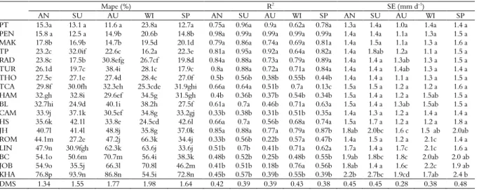
Table 1. Statistic performance of ETo methods in daily scale in relation to the Penman-Monteith method, considering the Accuracy (mean absolute percentage error, Mape), Precision (R2
), Tendency (systematic error, SE). Tukey´s test with significant minimum difference (DMS) at level of 5% probability for annual (AN), summer (SU), autumn (AU), winter (WI) and spring (SP) analysis. ETo´s models: Priestley-Taylor (PT), Penman (PEN), Makkink (MAK), Tanner-Pelton (TP), Radiation (RAD), Turc (TUR), Thornthwaite (THO), Class A pan (TCA), Hamon (HAM), Benevidez-Lopez (BL), Camargo (CAM), Hargreaves-Samani (HS), Jensen-Haise (JH), Romanenko (ROM), Linacre (LIN), Blaney-Criddle (BC), Jobson (JOB) and Kharrufa (KHA).
Mape (%) R2 SE (mm d-1)
AN SU AU WI SP AN SU AU WI SP AN SU AU WI SP
PT 15.3a 13.1 a 11.6 a 23.8a 12.7a 0.75a 0.96a 0.9a 0.62a 0.78a 1.3a 1.4a 1.0a 1.4a 1.4 a
PEN 15.8 a 12.5 a 14.9b 20.6b 14.8b 0.98a 0.99a 0.99a 0.99a 0.99a 1.4a 1.4a 1.1a 1.3a 1.5 a
MAK 17.8b 16.9b 14.7b 19.5d 20.1d 0.79a 0.86a 0.74a 0.69a 0.81a 1.4a 1.5a 1.1a 1.3 a 1.6 a
TP 23.2c 32.0if 22.6c 16.2a 22.3e 0.81a 0.95a 0.92a 0.64a 0.82a 1.4a 1.8ab 1.2a 1.1 a 1.5 a
RAD 23.8c 17.5b 30.8efg 26.7cf 19.8d 0.84a 0.88a 0.73a 0.79a 0.89a 1.4a 1.4 a 1.3ab 1.3 a 1.5 a
TUR 26.1d 19.7c 38.4i 28.1c 17.9c 0.8a 0.88a 0.72a 0.71a 0.84a 1.4a 1.4 a 1.4ab 1.3 a 1.4 a
THO 27.5e 27.1e 27.4d 28.4c 27.0f 0.5b 0.56b 0.38b 0.55b 0.44b 1.4a 1.4 a 1.1 a 1.3 a 1.5 a
TCA 29.8f 30.0fh 32.3eh 25.3cde 31.9ghi 0.66a 0.64a 0.51b 0.7a 0.13c 1.5a 1.5 a 1.2 a 1.2 a 1.6 a
HAM 32.gh 32.8i 29.6ef 34.5g 31.5gh 0.4b 0.36b 0.37b 0.54b 0.34b 1.5a 1.4 a 1.2 a 1.5ab 1.5 a
BL 32.7hi 24.9d 40.1i 38.2h 27.5f 0.61a 0.7a 0.46b 0.71a 0.63a 1.5a 1.4 a 1.3ab 1.5ab 1.5 a
CAM 33.9j 37.1k 30.5ef 34.8g 33.2gj 0.33b 0.38b 0.31b 0.51b 0.35a 1.4a 1.3 a 1.2 a 1.4 a 1.4 a
HS 35.6k 42.1l 33.8e 24.5cd 42.6l 0.66a 0.7a 0.56b 0.68a 0.74a 1.5a 1.7 a 1.2 a 1.2 a 1.8 a
JH 40.7l 41.4l 48.8j 35.8g 37.0k 0.85a 0.88a 0.77a 0.79a 0.87b 1.8ab 2.0bc 1.6 c 1.5 ab 2.0ab
ROM 44.1m 27.2e 47.2j 66.3k 34.4j 0.33b 0.56b 0.22b 0.57a 0.47b 1.4a 1.5 a 1.2 a 2.1c 1.4 a
LIN 47.9n 30.9fgh 62.3k 63.6j 33.6j 0.51b 0.7b 0.41b 0.71a 0.62a 1.7a 1.4 a 1.7c 2.1c 1.6 a
BC 54.1o 50.6m 70.7m 56.4i 38.3k 0.48b 0.52b 0.25b 0.48b 0.55b 1.9ab 1.8bc 1.8c 2.0ab 2.0 ab
JOB 54.9o 35.5j 66.3l 70.8l 46.2m 0.41b 0.51b 0.18b 0.76a 0.56b 1.8ab 1.4 a 1.6c 2.2c 1.9 ab
KHA 76.8p 93.9n 86.8n 54.5i 72.8n 0.45b 0.57b 0.39b 0.55b 0.39b 2.2b 2.7bc 1.9cd 1.7ab 2.4 b
DMS 1.34 1.55 1.77 1.98 1.64 0.42 0.39 0.39 0.43 0.38 0.45 0.45 0.28 0.38 0.48
In the summer, the PEN and PT methods were more accurate, with both having lower values of Mape (12.6 and 13.1%) and R2 (0.99 and 0.96). In
the autumn, the most accurate model was PT, followed by MAK and PEN, and the latter exhibited the same significance value according to Tukey’s test. The PT method showed lower Mape and ES (11.59% and 1.03 mm day-1), and the PEN method
showed the highest R2 (0.99).
In general, the accuracy of the analyzed models was not adequate for winter. Regardless, the evaluated methods with the best accuracy were TP, MAK and PEN. Despite the low R2 (0.62), the TP
model showed lower values of Mape and ES for this season: 16.20% and 1.08 mm day-1, respectively.
PEN, however, had the highest R2 among all models
(0.98). The MAK and PEN models exhibited low accuracy with Mape values of 19.52 and 20.59%, respectively, compared to that of the Penman-Monteith method.
For spring, the most accurate model was PT, followed by PEN and TUR, and PT showed the highest Mape value (12.67%) and one of the lowest ES values (1.34 mm day-1). For the PEN and TUR
models, the Mape (14.84 and 17.88%) was slightly higher than that of the PT model, and the ES values (1.55 and 1.43 mm day-1) were reasonable. The PEN
model had the highest R2 (0.99). These results are
different from those found by Pereira et al.(2009), who analyzed data from 2007 to 2008 and observed that the JH, RAD, PEN and BC methods are adequate for estimating reference evapotranspiration
on a daily scale, regardless of the season, in the Serra da Manriquiera region, Minas Gerais State. This dissimilar result is most likely because of the differences in climate and altitude between the regions.
The THO, HS and BL models were among the most accurate of those that only used temperature and relative humidity in their equations. For this study, the most accurate model for the whole year was THO (Mape = 27.5%), and the most accurate models were BL, THO, HS and THO, for summer, autumn, winter and spring, respectively. All of the models exhibited low values of ES and R2 (between
0.5 and 0.6).
The other models that were analyzed on a daily time scale did not show good accuracy. The Mape values were 17.5 and 93.9% using the RAD and KHA methods, respectively, for summer
The same estimated ETo methods were evaluated for periods of 5 days (Table 2). The model with the best accuracy was PT, followed by PEN and MAK. However, according to Tukey’s analysis, the latter two models performed similarly. The Mapes were 14.1, 15.9, and 16.1% for the PT, PEN and MAK models, respectively. The PT model showed the lowest SE (1.0 mm day-1), and the PEN
model had the highest R2 (0.98). Tagliaferre
Table 2. Statistic performance of ETo methods in 5-day scale in relation to the Penman-Monteith method, considering the Accuracy (mean absolute percentage error, Mape), Precision (R2
), Tendency (Systematic Error, SE). Tukey´s test with significant minimum difference (DMS) at level of 5% probability for annual (AN), summer (SU), autumn (AU), winter (WI) and spring (SP) analysis. ETo´s models: Priestley-Taylor (PT), Penman (PEN), Makkink (MAK), Tanner-Pelton (TP), Radiation (RAD), Turc (TUR), Thornthwaite (THO), Class A pan (TCA), Hamon (HAM), Benevidez-Lopez (BL), Camargo (CAM), Hargreaves-Samani (HS), Jensen-Haise (JH), Romanenko (ROM), Linacre (LIN), Blaney-Criddle (BC), Jobson (JOB) and Kharrufa (KHA).
Mape (%) R2 SE (mm d-1)
AN SU AU WI SP AN SU AU WI SP AN SU AU WI SP
PT 14.1a 12.5ab 10.2a 23.5 a 10.0 a 0.7a 0.96a 0.92a 0.59b 0.66a 1.0 a 1.1 a 0.9 a 1.2b 0.9 a
PEN 15.9b 12.4ab 15.0b 20.8f 15.2cd 0.98a 0.99a 0.99a 0.99a 0.99a 1.2 a 1.1 a 1 a 1.1 ab 1.1 a
MAK 16.1b 14.9cde 11.6 a 18.9cd 19.2hi 0.8a 0.82a 0.76a 0.76a 0.78a 1.2 a 1.1 a 0.9 a 1.1 ab 1.2 a
THO 18.3ef 15.5efg 17.4e 23.4 a 16.7k 0.57a 0.59a 0.47a 0.63a 0.44b 1.1 a 1.0 a 0.9 a 1.1 ab 1.1 a
TP 20.5c 31.9def 19.3c 11.5g 19.5def 0.78a 0.95a 0.94a 0.63a 0.76a 1.2 a 1.6b 1 a 0.8 a 1.2 a
RAD 21.3de 15.1l 28.7d 23.6 a 17.1i 0.83a 0.84a 0.71a 0.82a 0.89a 1.2 a 1.1 a 1.1 a 1.1ab 1.1 a
TCA 21.6ef 17.5def 25.4h 19.0g 24.4b 0.8a 0.83a 0.64a 0.87a 0.7a 1.2 a 1.2 a 1.0 a 1.0 a 1.3ab
TUR 22.0ef 15.5de 35.1f 23.4 a 13.1efg 0.8b 0.85b 0.73b 0.75a 0.82a 1.2 a 1.1a 1.2 a 1.1ab 1.0ab
CAM 22.0g 20.6bcd 20.9g 28.7i 17.6ghi 0.42b 0.33b 0.39b 0.62b 0.33b 1.1 a 1.0 a 1 a 1.3bc 0.9 a
HAM 22.4ef 19.9ghi 20.7d 29.6h 19.2fgh 0.47b 0.3b 0.46b 0.63a 0.29b 1.2 a 1.1 a 1.0 a 1.3bc 1.1ab
BL 24.3ef 14.4ghi 32.5d 31.7h 17.9hi 0.64a 0.76a 0.5b 0.78a 0.65a 1.2 a 1.0 a 1.1 a 1.3bc 1.1ab
HS 26.6h 32.1l 25.6e 16.1b 33.3m 0.71a 0.81a 0.57b 0.77a 0.8a 1.3 a 1.4ab 1 a 0.9 a 1.5b
JH 38.2i 38.7m 45.9i 32.9i 34.8m 0.85a 0.85a 0.77a 0.83a 0.85a 1.7b 1.8c 1.5b 1.4cd 1.7dc
LIN 38.9j 19.3k 54.6i 55.9n 24.0i 0.48b 0.77a 0.39b 0.77a 0.64a 1.5ab 1.1 a 1.6b 2.0d 1.3ab
ROM 41.2i 23.4fgh 44.9j 65.3l 30.4j 0.27b 0.56b 0.16c 0.6b 0.44b 1.1 a 1.2 a 1.1 a 2.0d 0.9 a
JOB 44.0l 21.5n 56.9l 61.6k 34.7m 0.37b 0.5b 0.09g 0.78a 0.62a 1.6b 1.1 a 1.5b 2.1d 1.6b
BC 50.7k 46.3ij 67.8k 52.8m 34.3m 0.35b 0.35b 0.11d 0.39b 0.43b 1.8bc 1.6b 1.7b 1.9d 1.7bc
KHA 62.6m 76.7 o 73.5m 42.4j 57.4n 0.54b 0.56b 0.54b 0.65a 0.38b 2.1c 2.5c 1.9bc 1.5cd 2.2c
DMS 1,58 2,05 1,76 1,84 1,62 0.4 0.34 0.39 0.36 0.38 0.29 0.28 0.27 0.25 0.29
For summer (Table 2), the models with better accuracy were PEN, PT and BL, with Mape values of 12.4, 12.5, and 14.4%, respectively. However, the PEN and BL models performed similarly according to Tukey’s test. The lowest tendency values were for the THO, BL and CAM models (1.0 mm day-1). For
autumn, the PT and MAK models exhibited the best accuracy, with lower values of Mape (10.2 and 11.6%, respectively). For both evaluations, the most precise method was PEN with an R2 of 0.99.
For winter, the TP model was much more accurate than the others, with an 11.5% Mape in addition to a lower value of ES (0.83 mm day-1). In
this case, HS was the second most accurate model, with a Mape of 16.1%. The HS model was also somewhat biased because the ES was 0.93 mm day-1.
Finally, in the spring, the model with the best accuracy was PT, followed by TUR, PEN and THO with Mapes of 10.0, 13.1, 15.2 and 16.7%, respectively, while the less tendentious models were PT, CAM and ROM, which all had an ES of 0.9 mm day-1.
THO was the most accurate of the models that only used temperature and relative humidity data for the annual and spring periods; BL was best for summer, HS was best for winter, and CAM was best for autumn. All the Mape values were higher than 14,4%.
The other models that were analyzed on a 5-day time scale did not show good accuracy. The Mape values were 14,4 and 76,7% for the BL and KHA methods, respectively, for summer.
When analyzing the same models using a biweekly scale (Table 3), the most accurate models
were PT, THO and MAK, with Mapes of 13.82, 15.33, and 15.62%, respectively. Despite the good accuracy, the models showed low precision compared to the PM model; the R2 values were 0.68,
0.64, and 0.79 for PT, THO and MAK, respectively. The methods with greater accuracy on a biweekly scale during the summer were THO and BL, followed by PT and PEN. The former two had Mapes of 10.56 and 11.25%, respectively, and both had the same low tendency (ES) of 0.74 mm day-1
and the same representativity, according to Tukey’s test. For autumn, the MAK and PT methods showed the lowest Mapes (9.7 and 9.8%, respectively) and the lowest ES values (0.8 and 0.7 mm day-1, respectively); both methods showed
similar results from Tukey’s test. For winter, the TP, HS and TCA, TP models exhibited better accuracy with a Mape of 9.68%, and the HS and TCA models showed low tendencies with ES values of 0.82 mm day-1 and 0.91 mm day-1, respectively.
Finally, for spring, the PT, CAM and TUR models were the most accurate. Among those models, the PT method showed the lowest values of Mape and ES: 8.70% and 0.62 mm day-1,
respectively.
Table 3. Statistic performance of ETo methods in 15-day scale in relation to the Penman-Monteith method, considering the Accuracy (mean absolute percentage error, Mape), Precision (R2
), Tendency (Systematic Error, SE). Tukey´s test with significant minimum difference (DMS) at level of 5% probability for annual (AN), summer (SU), autumn (AU), winter (WI) and spring (SP) analysis. ETo´s models: Priestley-Taylor (PT), Penman (PEN), Makkink (MAK), Tanner-Pelton (TP), Radiation (RAD), Turc (TUR), Thornthwaite (THO), Class A pan (TCA), Hamon (HAM), Benevidez-Lopez (BL), Camargo (CAM), Hargreaves-Samani (HS), Jensen-Haise (JH), Romanenko (ROM), Linacre (LIN), Blaney-Criddle (BC), Jobson (JOB) and Kharrufa (KHA).
Mape (%) R2 SE (mm d-1)
AN SU AU WI SP AN SU AU WI SP AN SU AU WI SP
PT 13.8abc 12.4bcde 9.8a 24.2g 8.7a 0.68a 0.94a 0.94a 0.54c 0.52b 0.9 a 0.8 a 0.7 a 1.1ab 0.6 a
THO 15.3bcd 10.6abc 14.3b 22.2f 13.9de 0.64a 0.57b 0.57b 0.71b 0.33b 1.0 a 0.7 a 0.8 a 1.0ab 0.8 a
MAK 15.6def 14.8ghi 9.7a 20.0d 18.3j 0.79a 0.65ab 0.78a 0.8b 0.70a 1.0 a 0.9 a 0.8 a 1.0ab 1.0ab
PEN 16.0ef 12.6cde 15.5b 20.7de 15.2efh 0.98a 0.99a 0.99a 0.99a 0.98a 1.0 a 0.8 a 0.8 a 1.0ab 0.9 a
CAM 17.5f 13.5defg 19.0c 26.4h 10.8b 0.52b 0.17d 0.45b 0.63c 0.25b 0.9 a 0.7 a 0.9 a 1.1ab 0.6 a
HAM 19.6gh 14.6fgh 18.9c 29.0i 15.9hi 0.54b 0.15d 0.54b 0.65b 0.17b 1.1 a 0.8 a 0.9 a 1.2b 0.9 a
TP 19.9gh 32.4l 17.5c 9.7ª 20.0k 0.77a 0.94a 0.96a 0.62c 0.65a 1.0 a 1.4ab 0.9 a 0.7 a 1.0ab
TCA 20.4hi 16.6i 24.3i 18.1c 22.7l 0.84a 0.78ab 0.71a 0.91a 0.67a 1.1 a 0.9 a 0.9 a 0.9 a 1.1ab
RAD 20.8hi 15.0ghi 29.0e 22.2f 16.7i 0.81a 0.71ab 0.75a 0.83b 0.85a 1.1 a 0.8 a 1.0 a 1.0ab 0.9 a
TUR 20.9hi 14.6fgh 35.6g 20.4de 12.0c 0.79a 0.71ab 0.46b 0.79b 0.76a 1.0 a 0.8 a 1.2ab 0.9 a 0.7 a
BL 22.1h 11.2bcd 32.5f 29.6i 14.2def 0.64a 0.75ab 0.56b 0.83b 0.54b 1.1 a 0.7 a 1.1ab 1.2b 0.8 a
HS 24.3j 28.9k 24.0d 14.6b 29.9n 0.75a 0.75ab 0.56b 0.82b 0.78a 1.1 a 1.2ab 0.9 a 0.8 a 1.3ab
LIN 36.5k 15.8hi 55.7j 53.1m 19.9k 0.4b 0.76ab 0.4b 0.76b 0.51b 1.4b 0.8a 1.6b 1.9c 1.0 ab
JH 37.7l 38.2m 45.9h 31.5j 35.0o 0.84a 0.72ab 0.8a 0.86b 0.79a 1.5b 1.6b 1.4b 1.3b 1.6b
JOB 40.5m 15.7hi 57j 59.6n 28.8n 0.33b 0.48c 0.08c 0.77b 0.54b 1.5b 0.8 a 1.5b 2.1d 1.3ab
ROM 40.7m 22.7j 47.7i 64.1o 27.3m 0.19b 0.56b 0.11c 0.55c 0.38b 1.0 a 1.0 a 1.0 a 1.9c 0.6 a
BC 49.7n 47.6n 66.5k 49.2l 34.2o 0.24b 0.15d 0.01d 0.33c 0.25b 1.7bc 1.5ab 1.6b 1.8c 1.5b
KHA 58.5o 72.4o 69.2l 39.6k 52.2p 0.61a 0.51c 0.58b 0.72b 0.28b 2.0 c 2.4c 1.8bc 1.4b 2.1c
DMS 1,93 1,93 1,77 1,70 1.15 0.37 0.36 0.37 0.34 0.40 0.25 0.33 0.30 0.23 0.32
The RAD method overestimates evapotranspiration to a greater degree in the summer-autumn period than in the spring-winter period. The TCA method overestimates reference evapotranspiration by 26% in summer-autumn period and by 24% in the winter-spring period relative to the values from the standard method of FAO (PM).
THO surpasses the models that use only temperature and relative humidity for summer and autumn. The best models were HS for winter and CAM for spring. The THO model was developed for a monthly scale and has better accuracy when the time scale changes from daily to biweekly, with Mapes of 27.49 and 15.33%, respectively. Confirming the report of Camargo and Camargo (2000), the Thornthwaite model is adequate for the wet climate regions of São Paulo State, independent of latitude and altitude.
In general, the models had a low tendency, not exceeding 2.7 mm day-1 for all scales. The PEN
model showed higher values of precision for all analyses.
The PT method, despite the high accuracy for all time scales, underestimated ETo in the winter (Figure 1) by up to 1.5 mm day-1, 2 mm day-1, and
2 mm day-1 for the daily, 5-day and biweekly scales,
respectively, when the ETo estimated by PM was approximately 5 mm day-1. Additionally, in the
summer, the PT model overestimates up to 1 mm on daily, 5-day and biweekly scales.
Therefore, the PT method is accurate for the summer, when the weather is hot and wet (Figure 1). However, the PT method is less precise for winter, when the climate is drier. During this
season, the Tanner and Pelton method can be applied because of the greater accuracy shown for all analyses in the winter.
Figure 1. Relation between ETo measured by the Priestley and Taylor method (PT) and ETo observed by the Penman and Monteith method (PM) in daily (A), 5-day (B) and 15-day (C) scales during summer and winter.
The other models that were analyzed on a 15-day time scale were not accurate. The Mape values were 15,0 and 72,4% using the RAD and KHA methods, respectively, for summer.
Conclusion
in the Jaboticabal region, SP, for all time scales. However, the methods of Penman and Makkink must not be dismissed.
Especially in the winter, the method of Tanner and Pelton is more accurate and less biased of all the methods.
Finally, the Thornthwaite method is the most accurate of those that only require temperature and relative humidity in equations for annual analysis.
References
ALLEN, R. G.; PEREIRA, L. S.; RAES, D.; SMITH, M.
Crop evapotranpiration: Guidelines for computing crop water requirements. Rome: FAO, 1998. (Irrigation and Drainage, Paper 56).
BENEVIDES, J. G.; LOPEZ, D. Formula para el caculo de la evapotranspiracion potencial adaptada al tropic (15º N - 15º S). Agronomia Tropical, v. 20, n. 5, p. 335-345, 1970.
BLANEY, H. F.; CRIDDLE, W. O. Determining water requirements in irrigated areas from climatological and irrigation data. Washington, D.C.: USDA Soil Conservation Service, 1950.
BORGES, A. C.; MENDIONDO, E. M. Comparação entre equações empíricas para estimativa da evapotranspiração de referência na Bacia do Rio Jacupiranga.Revista Brasileira de Engenharia Agrícola Ambiental, v. 11, n. 3, p. 293-300, 2007.
BOWIE, G. L.; MILLS, W. B.; PORCELLA, D. B.; CAMPBELL, C. L.; PAGENKOPF, J. R.; RUPP G. L.; JOHNSON, K. M.; CHAN, P. W. H.; GHERINI, S. A.; CHAMBERLIN, C. E. Rates, constants and kinetics formulations in surface water quality modeling.2nd ed. Athens: U.S. Environmental Protection Agency, Environmental Research Lab., 1985. (EPA/600/3-85/040). CAMARGO, A. P. Balanço hídrico no Estado de São Paulo. Campinas: Instituto Agronômico, 1971.
CAMARGO, A. P.; CAMARGO, M. B. P. Uma revisão analítica da evapotranspiração potencial.Bragantia, v. 59, n. 2, p. 125-137, 2000.
CAMARGO, A. P.; SENTELHAS, P. C. Avaliação do desempenho de difernets métodos de estimativa da evapotranspiração potencial no estado de São Paulo. Revista Brasileira de Agrometeorologia, v. 5, n. 1, p. 89-97, 1997.
CAVALCANTI JÚNIOR, E. G.; OLIVEIRA, A. D.; ALMEIDA, B. M.; ESPÍNOLA SOBRINHO, J. Métodos de estimativa da evapotranspiração de referência para as condições do semiárido Nordestino. Ciências Agrárias, v. 32, n. 1, p. 1699-1708, 2011.
DOORENBOS, J.; PRUITT, W. O. Guidelines for predicting crop water requirements. Rome: FAO, 1977.
HAMON, W. R. Estimating potential evapotranspiration.
Journal of Hydraulics Division ASCE, v. 87, n. 3, p. 107-120, 1961.
HARGREAVES, G. L.; SAMANI, Z. A. Reference crop evapotranspiration from temperature. Basin. Journal of the Irrigation and Drainage Division-ASCE, v. 111, n. 1, p. 113-124, 1985.
JENSEN, M. E.; HAISE, H. R. Estimating evapotranspiration from solar radiation. Journal of the Irrigation and Drainage Division-ASCE, v. 4, n. 1, p. 15-41, 1963.
JOBSON, H. E. Thermal modeling of flow in the San Diego Aqueduct, California, and its relation to evaporation. San Diego: US Geological Survey, 1980. KHARRUFA, N. S. Simplified equation for evapotranspiration in arid regions. Beitrage zur Hydrologie Sonderheft, v. 5, n. 1, p. 39-47, 1985.
LINACRE, E. T. A. Simple formula for estimating evaporation rates in various climates, using temperature data alone. Agricultural Meteorology, v. 18, n.1, p. 409-424, 1977.
MAKKINK, G. F. Testing the Penman formula by means of lysimeters. Journal of the Institution of Water Engineers, v. 11, n. 3, p. 277-288, 1957.
MEDEIROS, S. L. P. Avaliação de métodos de estimativa da evapotranspiração de referência para a região mesoclimática de Santa Maria-RS. Revista Brasileira de Agrometeorologia, v. 6, n. 1, p. 105-109, 1998.
MENDONÇA, E. A.; DANTAS, R. T. Estimativa da evapotranspiração de referência no município de Capim, PB. Revista Brasileira de Engenharia Agrícola Ambiental, v. 14, n. 2, p. 196-202, 2010.
MENDONÇA, J. C.; SOUZA, E. F.; SALASSIER, B.; DIAS, G. P.; GRIPPA, S. Comparação entre métodos de estimativa da evapotranspiração de referência (ET0) na região Norte Fluminense, RJ. Revista Brasileira de Engenharia Agrícola e Ambiental, v. 7, n. 2, p. 275-279, 2003.
OLIVEIRA, A. D.; VOLPE, C. A. Comparação de métodos de estimativa da evapotranspiração de referência, utilizando dados de estações meteorológicas convencional e automática. Revista Brasileira de Agrometeorologia, v. 11, n. 2, p. 253-260, 2003.
OLIVEIRA, G. Q.; LOPES, A. S.; JUNG, L. H.; NAGEL, P. L.; BERTIOLI, D. M. Desempenho de métodos de estimativa da evapotranspiração de referência baseadas na temperatura do ar, em Aquidauana-MS. Revista Brasileira de Agricultura Irrigada, v. 5, n. 3, p. 224-234, 2011.
PENMAN, H. L. Natural evaporation from open water, bare soil and grass. Proceedings of the Royal Society of London, v. 193, n. 1032, p. 120-145, 1948.
PEREIRA, A. R.; ANGELOCCI, L. R.; SENTELHAS, P. C. Agrometeorologia, fundamentos e aplicações práticas. Guaíba: Agropecuária, 2002.
PEREIRA, A. R.; NOVA, N. A. V.; SEDIYAMA, R.
Evapo(transpi)ração. Piracicaba: Fealq, 1997.
Reference evapotranspiration models in the Jaboticabal region 9
da Serra da Mantiqueira, MG. Ciência Rural, v. 39, n. 9, p. 2488-2493, 2009.
PRIESTLEY, C. H. B.; TAYLOR, R. J. On the assessment of the surface heat flux and evaporation using large-scale parameters. Monthly Weather Review, v. 100, n. 2, p. 81-92, 1972.
ROMANENKO, V. A. Computation of the autumn soil moisture using a universal relationship for a large area. Kiev: Proceedings Ukrainian Hydrometeorological Research Institute, 1961.
SOUZA, I. F.; SILVA, V. P. R.; SABINO, F. G.; NETTO, A. O. A.; SILVA, B. K. N; AZEVEDO, P. V. Evapotranspiração de referência nos perímetros irrigados do Estado de Sergipe. Revista Brasileira de Engenharia Agrícola e Ambiental, v. 14, n. 6, p. 633-644, 2010. SYPERRECK, V. L. G.; KLOSOWSKI, E. S.; GRECO, M.; FURLANETTO, C. Avaliação de desempenho de métodos para estimativas de evapotranspiração de referência para a região de Palotina, Estado do Paraná. Acta Scientiarum. Agronomy, v. 30, n. 5, p. 603-609, 2008.
TAGLIAFERRE, C.; SILVA, R. A. J.; ROCHA, F. A.; SANTOS, L. C.; SILVA, C. S. Estudo comparativo de diferentes metodologias para determinação da evapotranspiração de referência em Eunápolis, BA.
Caatinga, v. 23, n. 1, p. 103-111, 2010.
TANNER, C. O.; PELTON, W. L. Potential evapotranspiration estimates by the approximate energy balance method of Penman. Journal of Geophysical Research, v. 10, n. 65, p. 3391-3414, 1960.
THORNTHWAITE, C. W. An approach toward a rational classification of climate. Geographical Review, v. 38, n. 1, p. 55-94, 1948.
TURC, L. Estimation of irrigation water requirements, potential evapotranspiration: A simple climatic formula evolved up to date. Annals of Agronomy, v. 12, p. 13-49, 1961.
VESCOVE, H. V.; TURCO J. E. P.Comparação de três métodos de estimativa da evapotranspiração de referência para a região de Araraquara-SP. Engenharia Agrícola, v. 25, n. 3, p. 713-721, 2005.
XU, C. Y.; SINGH, V. P. Evaluation and generalization of temperature-based methods for calculating evaporation.
Hydrolological Processes, v. 15, n. 2, p. 305-319, 2001.
Received on August 17, 2012. Accepted on December 27, 2012.