A Constraint Programming Approach to Optimize Network Calls by Minimizing Variance in Data Availability Times

journals site: http://www.iariajournals.org

contact: petre@iaria.org

Responsibility for the contents rests upon the authors and not upon IARIA, nor on IARIA volunteers,

staff, or contractors.

IARIA is the owner of the publication and of editorial aspects. IARIA reserves the right to update the

content for quality improvements.

Abstracting is permitted with credit to the source. Libraries are permitted to photocopy or print,

providing the reference is mentioned and that the resulting material is made available at no cost.

Reference should mention:

International Journal on Advances in Telecommunications, issn 1942-2601 vol. 10, no. 1 & 2, year 2017, http://www.iariajournals.org/telecommunications/

The copyright for each included paper belongs to the authors. Republishing of same material, by authors

or persons or organizations, is not allowed. Reprint rights can be granted by IARIA or by the authors, and

must include proper reference.

Reference to an article in the journal is as follows:

International Journal on Advances in Telecommunications, issn 1942-2601

vol. 10, no. 1 & 2, year 2017, <start page>:<end page> , http://www.iariajournals.org/telecommunications/

IARIA journals are made available for free, proving the appropriate references are made when their

content is used.

Sponsored by IARIA

www.iaria.org

Editors-in-Chief

Tulin Atmaca, Institut Mines-Telecom/ Telecom SudParis, France

Marko Jäntti, University of Eastern Finland, Finland

Editorial Advisory Board

Ioannis D. Moscholios, University of Peloponnese, Greece

Ilija Basicevic, University of Novi Sad, Serbia

Kevin Daimi, University of Detroit Mercy, USA

György Kálmán, Gjøvik University College, Norway

Michael Massoth, University of Applied Sciences - Darmstadt, Germany

Mariusz Glabowski, Poznan University of Technology, Poland

Dragana Krstic, Faculty of Electronic Engineering, University of Nis, Serbia

Wolfgang Leister, Norsk Regnesentral, Norway

Bernd E. Wolfinger, University of Hamburg, Germany

Przemyslaw Pochec, University of New Brunswick, Canada

Timothy Pham, Jet Propulsion Laboratory, California Institute of Technology, USA

Kamal Harb, KFUPM, Saudi Arabia

Eugen Borcoci, University "Politehnica" of Bucharest (UPB), Romania

Richard Li, Huawei Technologies, USA

Editorial Board

Fatma Abdelkefi, High School of Communications of Tunis - SUPCOM, Tunisia Seyed Reza Abdollahi, Brunel University - London, UK

Habtamu Abie, Norwegian Computing Center/Norsk Regnesentral-Blindern, Norway Rui L. Aguiar, Universidade de Aveiro, Portugal

Javier M. Aguiar Pérez, Universidad de Valladolid, Spain Mahdi Aiash, Middlesex University, UK

Akbar Sheikh Akbari, Staffordshire University, UK

Ahmed Akl, Arab Academy for Science and Technology (AAST), Egypt Hakiri Akram, LAAS-CNRS, Toulouse University, France

Anwer Al-Dulaimi, Brunel University, UK Muhammad Ali Imran, University of Surrey, UK

Muayad Al-Janabi, University of Technology, Baghdad, Iraq

Jose M. Alcaraz Calero, Hewlett-Packard Research Laboratories, UK / University of Murcia, Spain Erick Amador, Intel Mobile Communications, France

Ermeson Andrade, Universidade Federal de Pernambuco (UFPE), Brazil Cristian Anghel, University Politehnica of Bucharest, Romania

Regina B. Araujo, Federal University of Sao Carlos - SP, Brazil Pasquale Ardimento, University of Bari, Italy

Tulin Atmaca, Institut Mines-Telecom/ Telecom SudParis, France Mario Ezequiel Augusto, Santa Catarina State University, Brazil Marco Aurelio Spohn, Federal University of Fronteira Sul (UFFS), Brazil Philip L. Balcaen, University of British Columbia Okanagan - Kelowna, Canada Marco Baldi, Università Politecnica delle Marche, Italy

Ilija Basicevic, University of Novi Sad, Serbia

Carlos Becker Westphall, Federal University of Santa Catarina, Brazil Mark Bentum, University of Twente, The Netherlands

David Bernstein, Huawei Technologies, Ltd., USA

Eugen Borcoci, University "Politehnica"of Bucharest (UPB), Romania Fernando Boronat Seguí, Universidad Politecnica de Valencia, Spain Christos Bouras, University of Patras, Greece

Martin Brandl, Danube University Krems, Austria Julien Broisin, IRIT, France

Dumitru Burdescu, University of Craiova, Romania

Andi Buzo, University "Politehnica" of Bucharest (UPB), Romania Shkelzen Cakaj, Telecom of Kosovo / Prishtina University, Kosovo Enzo Alberto Candreva, DEIS-University of Bologna, Italy

Rodrigo Capobianco Guido, São Paulo State University, Brazil Hakima Chaouchi, Telecom SudParis, France

Silviu Ciochina, Universitatea Politehnica din Bucuresti, Romania José Coimbra, Universidade do Algarve, Portugal

Hugo Coll Ferri, Polytechnic University of Valencia, Spain Noel Crespi, Institut TELECOM SudParis-Evry, France

Leonardo Dagui de Oliveira, Escola Politécnica da Universidade de São Paulo, Brazil Kevin Daimi, University of Detroit Mercy, USA

Gerard Damm, Alcatel-Lucent, USA

Francescantonio Della Rosa, Tampere University of Technology, Finland Chérif Diallo, Consultant Sécurité des Systèmes d'Information, France

Klaus Drechsler, Fraunhofer Institute for Computer Graphics Research IGD, Germany Jawad Drissi, Cameron University , USA

António Manuel Duarte Nogueira, University of Aveiro / Institute of Telecommunications, Portugal Alban Duverdier, CNES (French Space Agency) Paris, France

Nicholas Evans, EURECOM, France Fabrizio Falchi, ISTI - CNR, Italy

Mário F. S. Ferreira, University of Aveiro, Portugal

Bruno Filipe Marques, Polytechnic Institute of Viseu, Portugal Robert Forster, Edgemount Solutions, USA

John-Austen Francisco, Rutgers, the State University of New Jersey, USA Kaori Fujinami, Tokyo University of Agriculture and Technology, Japan

Shauneen Furlong , University of Ottawa, Canada / Liverpool John Moores University, UK Ana-Belén García-Hernando, Universidad Politécnica de Madrid, Spain

Bezalel Gavish, Southern Methodist University, USA Christos K. Georgiadis, University of Macedonia, Greece

Hock Guan Goh, Universiti Tunku Abdul Rahman, Malaysia Pedro Gonçalves, ESTGA - Universidade de Aveiro, Portugal

Valerie Gouet-Brunet, Conservatoire National des Arts et Métiers (CNAM), Paris Christos Grecos, University of West of Scotland, UK

Stefanos Gritzalis, University of the Aegean, Greece William I. Grosky, University of Michigan-Dearborn, USA Vic Grout, Glyndwr University, UK

Xiang Gui, Massey University, New Zealand

Huaqun Guo, Institute for Infocomm Research, A*STAR, Singapore Song Guo, University of Aizu, Japan

Kamal Harb, KFUPM, Saudi Arabia

Ching-Hsien (Robert) Hsu, Chung Hua University, Taiwan Javier Ibanez-Guzman, Renault S.A., France

Lamiaa Fattouh Ibrahim, King Abdul Aziz University, Saudi Arabia Theodoros Iliou, University of the Aegean, Greece

Mohsen Jahanshahi, Islamic Azad University, Iran Antonio Jara, University of Murcia, Spain

Carlos Juiz, Universitat de les Illes Balears, Spain Adrian Kacso, Universität Siegen, Germany György Kálmán, Gjøvik University College, Norway

Eleni Kaplani, Technological Educational Institute of Patras, Greece Behrouz Khoshnevis, University of Toronto, Canada

Ki Hong Kim, ETRI: Electronics and Telecommunications Research Institute, Korea Atsushi Koike, Seikei University, Japan

Ousmane Kone, UPPA - University of Bordeaux, France Dragana Krstic, University of Nis, Serbia

Archana Kumar, Delhi Institute of Technology & Management, Haryana, India Romain Laborde, University Paul Sabatier (Toulouse III), France

Massimiliano Laddomada, Texas A&M University-Texarkana, USA

Wen-Hsing Lai, National Kaohsiung First University of Science and Technology, Taiwan Zhihua Lai, Ranplan Wireless Network Design Ltd., UK

Jong-Hyouk Lee, INRIA, France

Wolfgang Leister, Norsk Regnesentral, Norway

Elizabeth I. Leonard, Naval Research Laboratory - Washington DC, USA Richard Li, Huawei Technologies, USA

Jia-Chin Lin, National Central University, Taiwan Chi (Harold) Liu, IBM Research - China, China

Diogo Lobato Acatauassu Nunes, Federal University of Pará, Brazil

Andreas Loeffler, Friedrich-Alexander-University of Erlangen-Nuremberg, Germany Michael D. Logothetis, University of Patras, Greece

Renata Lopes Rosa, University of São Paulo, Brazil

Hongli Luo, Indiana University Purdue University Fort Wayne, USA Christian Maciocco, Intel Corporation, USA

Zoubir Mammeri, IRIT - Paul Sabatier University - Toulouse, France Herwig Mannaert, University of Antwerp, Belgium

Michael Massoth, University of Applied Sciences - Darmstadt, Germany Adrian Matei, Orange Romania S.A, part of France Telecom Group, Romania Natarajan Meghanathan, Jackson State University, USA

Emmanouel T. Michailidis, University of Piraeus, Greece Ioannis D. Moscholios, University of Peloponnese, Greece Djafar Mynbaev, City University of New York, USA Pubudu N. Pathirana, Deakin University, Australia Christopher Nguyen, Intel Corp., USA

Lim Nguyen, University of Nebraska-Lincoln, USA Brian Niehöfer, TU Dortmund University, Germany

Serban Georgica Obreja, University Politehnica Bucharest, Romania Peter Orosz, University of Debrecen, Hungary

Patrik Österberg, Mid Sweden University, Sweden Harald Øverby, ITEM/NTNU, Norway

Tudor Palade, Technical University of Cluj-Napoca, Romania Constantin Paleologu, University Politehnica of Bucharest, Romania Stelios Papaharalabos, National Observatory of Athens, Greece Gerard Parr, University of Ulster Coleraine, UK

Ling Pei, Finnish Geodetic Institute, Finland Jun Peng, University of Texas - Pan American, USA Cathryn Peoples, University of Ulster, UK

Dionysia Petraki, National Technical University of Athens, Greece Dennis Pfisterer, University of Luebeck, Germany

Timothy Pham, Jet Propulsion Laboratory, California Institute of Technology, USA Roger Pierre Fabris Hoefel, Federal University of Rio Grande do Sul (UFRGS), Brazil Przemyslaw Pochec, University of New Brunswick, Canada

Anastasios Politis, Technological & Educational Institute of Serres, Greece Adrian Popescu, Blekinge Institute of Technology, Sweden

Neeli R. Prasad, Aalborg University, Denmark

Dušan Radović, TES Electronic Solutions, Stuttgart, Germany Victor Ramos, UAM Iztapalapa, Mexico

Gianluca Reali, Università degli Studi di Perugia, Italy Eric Renault, Telecom SudParis, France

Leon Reznik, Rochester Institute of Technology, USA

Joel Rodrigues, Instituto de Telecomunicações / University of Beira Interior, Portugal David Sánchez Rodríguez, University of Las Palmas de Gran Canaria (ULPGC), Spain Panagiotis Sarigiannidis, University of Western Macedonia, Greece

Michael Sauer, Corning Incorporated, USA Marialisa Scatà, University of Catania, Italy

Zary Segall, Chair Professor, Royal Institute of Technology, Sweden Sergei Semenov, Broadcom, Finland

Mariusz Skrocki, Orange Labs Poland / Telekomunikacja Polska S.A., Poland Leonel Sousa, INESC-ID/IST, TU-Lisbon, Portugal

Cristian Stanciu, University Politehnica of Bucharest, Romania Liana Stanescu, University of Craiova, Romania

Cosmin Stoica Spahiu, University of Craiova, Romania

Young-Joo Suh, POSTECH (Pohang University of Science and Technology), Korea Hailong Sun, Beihang University, China

Jani Suomalainen, VTT Technical Research Centre of Finland, Finland Fatma Tansu, Eastern Mediterranean University, Cyprus

Ioan Toma, STI Innsbruck/University Innsbruck, Austria Božo Tomas, HT Mostar, Bosnia and Herzegovina Piotr Tyczka, ITTI Sp. z o.o., Poland

John Vardakas, University of Patras, Greece

Andreas Veglis, Aristotle University of Thessaloniki, Greece Luís Veiga, Instituto Superior Técnico / INESC-ID Lisboa, Portugal Calin Vladeanu, "Politehnica" University of Bucharest, Romania Benno Volk, ETH Zurich, Switzerland

Krzysztof Walczak, Poznan University of Economics, Poland Krzysztof Walkowiak, Wroclaw University of Technology, Poland Yang Wang, Georgia State University, USA

Yean-Fu Wen, National Taipei University, Taiwan, R.O.C. Bernd E. Wolfinger, University of Hamburg, Germany

Riaan Wolhuter, Universiteit Stellenbosch University, South Africa Yulei Wu, Chinese Academy of Sciences, China

Mudasser F. Wyne, National University, USA

Gaoxi Xiao, Nanyang Technological University, Singapore Bashir Yahya, University of Versailles, France

Abdulrahman Yarali, Murray State University, USA Mehmet Erkan Yüksel, Istanbul University, Turkey Pooneh Bagheri Zadeh, Staffordshire University, UK Giannis Zaoudis, University of Patras, Greece

Liaoyuan Zeng, University of Electronic Science and Technology of China, China Rong Zhao , Detecon International GmbH, Germany

Zhiwen Zhu, Communications Research Centre, Canada

Martin Zimmermann, University of Applied Sciences Offenburg, Germany Piotr Zwierzykowski, Poznan University of Technology, Poland

CONTENTS

pages: 1 - 10

Interference Suppression and Signal Detection for LTE and WLAN Signals in Cognitive Radio Applications Johanna Vartiainen, Centre for Wireless Communications, University of Oulu, Finland

Risto Vuohtoniemi, Centre for Wireless Communications, University of Oulu, Finland

Attaphongse Taparugssanakorn, Telecommunications Asian Institute of Technology, Thailand Natthanan Promsuk, Telecommunications Asian Institute of Technology, Thailand

pages: 11 - 21

Impact of Analytics and Meta-learning on Estimating Geomagnetic Storms: A Two-stage Framework for Prediction

Taylor K. Larkin, The University of Alabama, United States Denise J. McManus, The University of Alabama, United States pages: 22 - 37

Near Capacity Signaling over Fading Channels using Coherent Turbo Coded OFDM and Massive MIMO Kasturi Vasudevan, IIT Kanpur, India

pages: 38 - 49

Modelling and Characterization of Customer Behavior in Cellular Networks Thomas Couronn ́e, France Telecom R&D, France

Valery Kirzner, Institute of Evolution University of Haifa, Israel Katerina Korenblat, Ort Braude College, Israel

Elena Ravve, Ort Braude College, Israel Zeev Volkovich, Ort Braude College, Israel pages: 50 - 59

A Constraint Programming Approach to Optimize Network Calls by Minimizing Variance in Data Availability Times

Luis Neto, ISR-P, Instituto de Sistemas e Robótica - Porto, Portugal, Portugal

Henrique Lopes Cardoso, LIACC, Laboratório de Inteligência Artificial e Ciência de Computadores, Portugal Carlos Soares, INESC TEC, Instituto de Engenharia de Sistemas e Computadores, Tecnologia e Ciência, Portugal Gil Gonçalves, ISR-P, Instituto de Sistemas e Robótica - Porto, Portugal, Portugal

pages: 60 - 71

Microarea Selection Method for Broadband Infrastructure Installation Based on Service Diffusion Process Motoi Iwashita, Chiba Institute of Technology, Japan

Akiya Inoue, Chiba Institute of Technology, Japan Takeshi Kurosawa, Tokyo University of Science, Japan

Ken Nishimatsu, NTT Network Technology Laboratories, Japan pages: 72 - 84

An Improved Preamble Aided Preamble Structure Independent Coarse Timing Estimation Method for OFDM Signals

Soumitra Bhowmick, IIT, Kanpur, India Kasturi Vasudevan, IIT, Kanpur, India

Interference Suppression and Signal Detection for LTE and WLAN Signals in Cognitive

Radio Applications

Johanna Vartiainen

and Risto Vuohtoniemi

Centre for Wireless Communications University of Oulu Oulu, Finland Email: johanna.vartiainen@oulu.fi Email: risto.vuohtoniemi@oulu.fi

Attaphongse Taparugssanagorn

and Natthanan Promsuk

School of Engineering and Technology ICT Department, Telecommunications

Asian Institute of Technology (AIT) Pathum Thani, Thailand Email: attaphongset@ait.asia

Email: st117805@ait.asia

Abstract—Cognitive radio spectrum is traditionally divided into two spaces. Black space is reserved to primary users trans-missions and secondary users are able to transmit in white space. To get more capacity, black space has been divided into black and grey spaces. Grey space includes interfering signals coming from primary and other secondary users, so the need for interference suppression has grown. Novel applications like Internet of Things generate narrowband interfering signals. In this paper, the performance of the forward consecutive mean excision algorithm (FCME) method is studied in the presence of narrowband interfering signals. In addition, the extension of the FCME method called the localization algorithm based on double-thresholding (LAD) method that uses three thresholds is proposed to be used for both narrowband interference suppression and intended signal detection. Both Long Term Evolution (LTE) signal simulations and real-world LTE and Wireless Local Area Network (WLAN) signal measurements were used to verify the usability of the methods in future cognitive radio applications.

Keywords–interference suppression; signal detection; grey zone; cognitive radio; measurements.

I. INTRODUCTION

Heavily used spectrum calls for new technologies and in-novations. Novel applications and signals like Long Term Evo-lution (LTE) generate novel interfering environments like dis-cussed in COCORA 2016 [1]. Cognitive radio (CR) [2][3][4] [5][6][7] offers possibility to effective spectrum usage allowing secondary users (SU) to transmit at unreserved frequencies if they guarantee that primary users (PU) transmissions are not disturbed. Earlier, spectrum was divided into two zones (spaces): black and white zone. As black zone was fully reserved to PUs and off limits to secondary users, their transmission was allowed in white zones where there were no PU transmissions. The problem in this classification is that if the spectrum is not totally unused, secondary users are not able to transmit. Thus, the spectrum usage is not as efficient as it could be. Instead, spectra can be divided into three zones: white, grey (or gray) and black zone [8]. In this model, the SU transmission is allowed in white and grey spaces, as black spaces are reserved for PUs.

Cognitive radio has several novel applications. Long Term Evolution Advanced (LTE-A) is a 4G mobile

communica-tion technology [9]. LTE for M2M communicacommunica-tion (LTE-M) exploits cognitive radio technology and utilizes flexible and intelligent spectrum usage. Its focus is on high capacity. LTE-A enables one of the newest topics called Wide LTE-Area Internet of Things (IoT) [10], where sensors, systems and other smart devices are connected to Internet. Therein, long-range commu-nication, long battery life and minimal amount of data, as well as narrow bandwidth are key issues. IoT (or, widely thinking, Network of Things, NoT [11]) is already here. However, there are several problems and challenges. Many IoT devices use already overcrowded unlicensed bands. Another possibility is to use operated mobile communication networks but it wastes financial/frequency resources and technologies like 3G and LTE do not support IoT directly. Secondly, radio networks come more and more complex. Self-organized networks (SON) [12] form a key to manage complex IoT networks. One of the existing SON solutions is LTE standard. However, SON has no intelligent learning aka cognitivity. Cognitive IoT (CIoT) term has been proposed to highlight required intelligence [13][14]. CIoT can be considered to be a technological revolution that brings a new era of communication, connectivity and comput-ing. It has been predicted that by 2020, there are billions of connected devices in the world [15]. Thus, cognitivity is really needed.

As cognitive radio technology offers more efficient spec-trum use, there are many challenges. One of those is that the cognitive world is an interference-intensive environment. Especially in-band interfering signals cause problems. There are three main types of interference in CR: from SU to PU (SU-PU interference), from PU to SU (PU-SU interference), and interference among SUs (SU-SU interference) [16][17]. The basic idea in CR is that SU must not interfere PUs, so there should not be SU-PU interference. Instead, SU may be interfered by PUs or other SUs. When there are multiple PUs and SUs with different applications and technologies, cumulative interference is a problematic task [18]. In grey spaces, there is interference from PU (and possible other SU) transmissions. It is efficient to mitigate unknown interference in order to achieve higher capacity. Therefore, interference suppression (IS) methods are needed.

It is crystal clear that when operating in real-world with mobile devices and varying environment, computational com-plexity is one of the key issues. Fast and reliable as well as cost-effective, powersave and adaptive methods are needed. Thus, it is beneficial if one method does several operations. In this paper, a transform domain IS method called the forward consecutive mean excision (FCME) algorithm [19][20] is used for interfering signal suppression (IS) in cognitive radio ap-plications [1]. Its extension called the localization algorithm based on double-thresholding (LAD) method [21][22] can be used for intended signal detection. Both the methods detect all kind of signals regardless of their modulation types. The difference is that the LAD method is more accurate and, thus, suitable for detection. Thus, the extended LAD method that uses three thresholds is proposed to be used for both interference suppression and intended signal detection. The FCME algorithm and the LAD method are blind constant false alarm rate (CFAR) -type methods that are able to find all kind of relatively narrowband (RNB) signals in all kind of environments and in all kind of frequency areas. Here, RNB means that the suppressed signal is narrowband with respect to the studied bandwidth. The wider the studied band is the wider the suppressed signal can be.

First, future cognitive radio applications and interference environment in cognitive radios are considered. Focus is on IS in SU receiver interfered by PUs and other SUs. A scenario that clarifies the interference environment is presented and IS methods are discussed. The FCME algorithm and LAD methods are presented and those feasibilities are considered. Simulations for LTE-signals are used to verify the performance of the extended LAD method that uses three thresholds. Mea-surement results for LTE and Wireless Local Area Network (WLAN) signals are used to verify the performance of the FCME IS method.

This paper is organized as follows. The state of art is discussed in Section II. Section III focuses on interference environment in cognitive radios as Section IV considers in-terference suppression. The FCME algorithm and the LAD method are presented and their feasibility is considered in Section V. Simulation and measurement results are presented in Section VI. Conclusions are drawn in Section VII.

II. STATE OF THEART

Future applications that use cognitive approach include, for example, LTE-A and cognitive IoT [23][24]. LTE-A is an advanced version of LTE. Therein, orthogonal Frequency Division Multiplex (OFDM) signal is used. In OFDM systems, data is divided between several closely spaced carriers. LTE downlink uses OFDM signal as uplink uses Single Carrier Frequency Division Multiple Access (SC-FDMA). Downlink signal has more power than uplink signal. Thus, its interference distance is larger than uplink signals. OFDM offers high data bandwidths and tolerance to interference. As LTE uses 6 bandwidths up to 20 MHz, LTE-A may offer even 100 MHz bandwidth. LTE-A offers about three times greater spectrum efficiency when compared to LTE. In addition, some kind of cognitive characteristics are expected [25][26][27]. RNB interfering signals exist especially at grey zones. This calls for IS.

In the network ecosystem, it is expected that cognitive IoT [28][29] will be the next ’big’ thing to focus on.

Wide-area IoT is a network of nodes like sensors and it offers connections between/to/from systems and smart devices (i.e., objects) [10][30]. Cognitive IoT enables objects to learn, think and understand both the physical and social world. Connected objects are intelligent and autonomous and they are able to interact with environment and networks so that the amount of human intervention is minimized. Basically, a human cognition process is integrated into IoT system design. Technically, CIoT operates as a transparent bridge between the social and physical world. The radio platform in CIoT devices should be efficient, simple, agile and have low power. CIoT has several advantages, including time, money and effort saving while resource efficiency is increased. It offers adaptable and simple automated systems. CIoT will consist of numerous heteroge-neous, interconnected, embedded and intelligent devices that will generate a huge amount of data. The long-range (even tens of kilometers) connection of nodes via cellular connections is expected. Data sent by nodes is minimal and transmissions may seldom occur. Thus, there is no need to use wide bandwidths for a transmission. This saves power consumption but also spectrum resources.

Proposed technologies include, e.g., LoRa (’long range’) [31], Neul (’cloud’ in English) [32], Global System for Mobile (GSM), SigFox [33], and LTE-M [34]. As Neul is able to operate in bands below 1 GHz and LoRa as well as SigFox operate in ISM band, LTE-M operates in LTE frequencies. In SigFox, messages are 100 Hz wide. In Neul, 180 kHz band is needed. A common thing is that the ultra-narrowband (UNB) signals are proposed to be used. For example, LTE-M (BW 1.4 MHz) and narrowband IoT (NB-IoT) in LTE bands (BW 200 kHz) are studied. In LTE-M, maximum transmit power is of the order of 20 dBm. In the Third-Generation Partnership Project’s (3GPP) Radio Access Network Plenary Meeting 69, it was decided to standardize narrowband IoT [35][36]. Most of those technologies are on the phase of development. In any case, it is expected that the amount of narrowband signals is growing. Thus, IS is required, especially when it is operated in mobile bands.

III. INTERFERENCEENVIRONMENT INCR The received discrete-time signal is assumed to be of form

r(n) = m X i=1 si(n) + p X j=1 ij(n) + η, n ∈ Z, (1)

where si(n) is the ith intended (relatively) narrowband signal,

ij(n) is the jth unknown (relatively) narrowband interfering

signal, m is the number of intended signals, p is the number of interfering signals, and η is a complex additive white Gaussian noise (AWGN) with variance σ2

η. Here, relatively narrowband

signal means that the joint bandwidth of the intended and interfering signal(s) is less than 80% of the total bandwidth, so the FCME method is able to operate [19].

In modern CR, the spectrum is divided into three zones - white, grey and black. In Figure 1, zone classification is presented. It is assumed that PU-SU distance is >y km in the white zone, <x km in the black zone, and in the grey zone it holds that x km <PU-SU-distance <y km [37]. It means that if SU is more than y km from the PU, SU is allowed to transmit. If SU is closer than y km but further than x km from the PU, SU may be able to transmit with low power. Spectrum sensing

y-z km x-y km 0-x km y km z km x km black zone grey zone white zone 0 km

Figure 1: White, grey and black zones.

is required before transmission and there are interfering signals so IS is needed to ensure SU transmissions. If PU-SU distance is less than x km, SU transmission is not allowed.

Interference environment differs between the zones. White space contains only noise. Therein, the noise is most com-monly additive white Gaussian (AWGN) noise at the receiver’s front-end, and man-made noise. This is related to the used fre-quency band. Grey space contains interfering signals within the noise, which causes challenges. Grey space is occupied by PU (and possible other SU) signals with low to medium power that means interference with low to medium power. IS is required especially is this zone. Black space includes communications signals, possible interfering signals, and noise. In black space, there are PU signals with high power and SUs have no access. There must be some rules that enable SUs to transmit in grey zone without causing any harm to PUs. According to [38], SU can transmit at the same time as PU if the limit of inter-ference temperature at the desired receiver is not reached. In [3], it is considered the maximum amount of interference that a receiver is able to tolerate, i.e., an interference temperature model. This can be used when studying interference from SU to PU network. In [39], primary radio network (PRN) defines some interference margin. This can be done based on channel conditions and target performance metric. Interference margin is broadcasted to the cognitive radio network. In any case, the maximum transmit power of SUs is limited.

In our scenario presented in Figure 2, it is assumed that we have one PU base station (BS), several PU mobile stations and several SUs. SU terminals form microcells. Part or all of SUs are mobile and part of SUs may be intelligent devices or sensors (i.e., IoT). Between SUs, weak signal powers are needed for a transmission. One microcell can consist of, for example, devices in an office room. They can use the same or different signal types than PU. For example, in the office room case, WLAN can be used. Between the intelligent devices (IoT), UNB signals are used. It is assumed that SUs operate at grey zone, so IS is required to ensure the quality of SU transmissions.

SUs measure signals transmitted by PU base stations and estimate relative distance to them. Using this information, SUs know whether their short range communication will cause harmful interference to the PU base station. To enable secondary transmissions under continuous interference caused by the PU base station this interference is attenuated by IS.

The secondary access point knows the locations of PU terminals or SUs measure the power levels of the signals

Figure 2: Scenario with one macrocell and two microcells.

coming from PU mobile terminals in the uplink. If it is assumed that SUs know the locations of PUs, SUs do not interfere with PUs. If SUs do not know PUs locations, their transmission is allowed when received PU signal power is below some predetermined threshold. If the level of the power coming from a certain primary terminal is small, it is assumed that secondary transmission generates negligible interference towards primary terminal. However, it may happen that SUs don’t sense closely spaced silent PUs.

Let us consider microcell 1 in Figure 2. There are one SU transmitter SU TX1 and four terminals SU i, i = 1, · · · , 4. In addition to the intended signal from SU TX1, SU 1 receives the noise η, SU 2 receives PU downlink (PU BS) signal and the noise η, SU 3 receives PU downlink (PU BS) and PU uplink (PU 1) signals and the noise η, and SU 4 receives PU downlink (PU BS) signal, signal from other microcell’s SU, and the noise η. That is, we get from (1) that

r1(n) = s(n) + η, (2) r2(n) = s(n) + i2(n) + η, (3) r3(n) = s(n) + 2 X j=1 ij(n) + η, (4) r4(n) = s(n) + 3 X j=2 ij(n) + η, (5)

where i1(n) is PU 1, i2(n) is PU BS and i3(n) is other SU. For

example, if it is assumed that PUs are in the LTE-A network and SUs use WLAN signals, receiver SU 2 has to suppress OFDM signal, receiver SU 3 has to suppress OFDM and SC-FDMA signals, and receiver SU 4 has to suppress OFDM and WLAN signals.

In addition, interfering and communication (intended) sig-nals have to be separated from each other. The receiver has to

know what signals are interfering signals to be suppressed and what signals are of interest. In an ideal situation, detected and interfering signals have distinct characteristics. However, this is not always the situation. An easy way to separate an interfering signal from the intended signal is to use different bandwidths. For example, in LTE networks, it is known that there are 6 different signal bandwidths between 1.4 and 20 MHz that are used [9]. Especially if a different signal type is used, it is easy to separate interfering signals from our information signal. It can also be assumed that interfering signal has higher power than the desired signal. However, this consideration is out of the scope of this paper.

IV. INTERFERENCESUPPRESSION

Interference suppression exploits the characteristics of desired/interfering signal by filtering the received signal [40]. After 1970, IS techniques have been widely studied. IS techniques include, for example, filters, cyclostationar-ity, transform-domain methods like wavelets and short-time Fourier transform (STFT), high order statistics, spatial process-ing like beamformprocess-ing and joint detection/multiuser detection [41]. Filter-based IS is performed in the time domain. Those can be further divided into linear and nonlinear methods. Opti-mal filter (Wiener filter) can be defined only if the interference and signal of interest are known by their Power Spectral Den-sities (PSDs), which is only possible when they are stationary. Usually, the signal, the interference or both are nonstationary, so adaptive filtering is the alternative capable of tracking their characteristics. Linear predictive filters can be made adaptive using, for example, the least mean square (LMS) algorithm. In filter-based IS, both computational complexity and hardware costs are low but co-channel interference cannot be suppressed, and no interference with similar waveforms to signals can be suppressed. Cyclostationarity based IS has low hardware complexity but medium computational complexity. This may cause challenges in real-time low-power applications.

In transform domain IS [42], signal is suppressed in frequency or in some other transform domain (like fractional Fourier transform). Usually, frequency domain is used, so signal is transformed using the Fourier transform. Computa-tional complexity is medium, but transform domain IS cannot be used when interference and signal-of-interest have the same kind of waveforms and spectral power concentration. However, waveform design may be used. Transform domain IS has low hardware complexity. High-order statistics based IS is computationally complex, and multiple antennas/samplers are needed, so its hardware cost is high and computational complexity too. In beamforming, co-channel interference as well as interference with similar waveforms to the signal of interest can be suppressed, but because of multiple antennas, the hardware cost is high. Its computational complexity is medium.

The less about the interfering signal characteristics is known, the more demanding the IS task will be. As most of the IS methods need some information about the suppressed signals and/or noise, there are some methods that are able to operate blindly [19]. Blind IS methods do not need any a priori information about the interfering signals, their modulations or other characteristics. Also, the noise level can be unknown, so it has to be estimated. Blind IS methods are well suited for demanding and varying environments.

V. THEFCMEAND THELADMETHODS

The adaptively operating FCME method [19] was orig-inally proposed for impulsive IS in the time domain. It was noticed later that the method is practical also in the frequency domain [20]. Earlier, the FCME method has mainly been studied against sinusoidal and impulsive signals that are narrowband ones. The computational complexity of the FCME method is N log2(N ) due to the sorting [20]. Analysis of the

FCME method has been presented in [20].

The FCME method adapts according to the noise level, so no information about the noise level is required. Because the noise is used as a basis of calculation, there is no need for information about the suppressed signals. Even though it is assumed in the calculation that the noise is Gaussian, the FCME method operates even if the noise is not purely Gaussian [20]. In fact, it is sufficient that the noise differs from the signal. When it is assumed that the noise is Gaussian, x2 _{(=the energy of samples) has a chi-squared distribution}

with two degrees of freedom. Thus, the used IS threshold is calculated using [19]

Th= −ln(PF A,DES)x2= TCM Ex2, (6)

where TCM E = −ln(PF A,DES) is the used pre-determined

threshold parameter [20], PF A,DES is the desired false alarm

rate used in constant false alarm rate (CFAR) methods, x2₌ 1 Q Q X i=1 |xi|2 (7)

denotes the average sample mean, and Q is the size of the set. For example, when it is selected that PF A,DES = 0.1

(=10% of the samples are above the threshold in the noise-only case), the threshold parameter TCM E= −ln(0.1) = 2.3.

In cognitive radio related applications, controlling PF A,DESis

important, because PF A,DES is directly related to the loss of

spectral opportunities and caused interference [20]. Selection of proper PF A,DES values is discussed more detailed in [20].

The FCME method rearranges the frequency-domain samples in an ascending order according to the sample energy, selects 10% of the smallest samples to form the set Q, and calculates the mean of Q. After that, (6) is used to calculate the first threshold. Then, Q is updated to include all the samples below the threshold, a new mean is calculated, and a new threshold is computed. This is continued until there are no new samples below the threshold. Finally, samples above the threshold are from interfering signal(s) and suppressed.

The FCME algorithm is blind and it is independent of modulation methods, signal types and amounts of signals. It can be used in all frequency areas, from kHz to GHz. The only requirements are that (1) the signal(s) can not cover the whole bandwidth under consideration, and (2) the signal(s) are above the noise level. The first requirement means that the FCME method can be used against RNB signals. For example, 10 MHz signal is wideband when the studied bandwidth is that 10 MHz, but RNB when the studied bandwidth is, e.g., 100 MHz. In fact, it is enough that the interfering signal does not cover more than 80% of the studied bandwidth. However, the narrower the interference is, the better the FCME method operates [43].

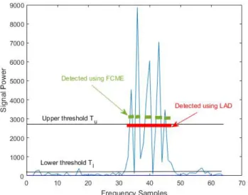
The LAD method [21] uses two FCME-thresholds in order to enhance the detection capability of the FCME method

Figure 3: Detection difference between the FCME and LAD methods. The LAD method finds one signal, as FCME finds five.

Figure 4: The LAD and LAD ACC methods.

[20]. One threshold is enough for interference suppressing, but causes problems in intended signal detection. If the threshold is too low, too much are detected. Instead, if the threshold is too high, not all the intended signals are detected. In the LAD method, the FCME algorithm is run twice with two different threshold parameters

TCM E1= −ln(PF A,DES1) (8)

and

TCM E2= −ln(PF A,DES2) (9)

in order to get two thresholds,

Tu= TCM E1x2j (10)

and

Tl= TCM E2x2l. (11)

Selection of proper values of PF A,DES1 and PF A,DES2 is

presented in [20] and in references therein. Usually, TCM E1=

13.81 (PF A,DES1= 10−4) and TCM E2= 2.66 (PF A,DES2=

0.07) are used [20].

After having two thresholds, a clustering is performed. Therein, adjacent samples above the lower threshold are grouped to form a cluster. If the largest element of that cluster exceeds the upper threshold, the cluster is accepted and decided to correspond a signal. Otherwise the cluster is rejected and decided to contain only noise samples. The detection difference between the FCME and LAD methods is illustrated in Figure 3. There is one raised cosine binary phase shift keying (RC-BPSK) signal whose bandwidth is 20% of the total bandwidth and signal-to-noise ratio (SNR) is 10 dB. The LAD method is able to find one signal. Instead, the FCME algorithm finds 5 signals if the upper threshold is used. If the FCME algorithm uses some other lower threshold, it still finds at least 5 signals because of the fluctuation of the signal.

The LAD method with adjacent cluster combining (ACC) [44] enhances the performance of the LAD method. Therein, if two or more accepted clusters are separated by at most p samples below the lower threshold, the accepted clusters are combined together to form one signal. The value of p is, for example, 1, 2 or 3 [20]. This enhances the correctly detected number of signals as well as bandwidth estimation accuracy of the LAD method [22]. In Figure 4, there are two RC-BPSK signals whose bandwidths are 5 and 8% of the total bandwidth. SNRs are 5 and 4 dB. The LAD method finds four signals, as the LAD ACC method finds two signals.

When considering IS, the LAD lower threshold may be too low thus suppressing too much. In addition, the LAD upper threshold may be too high thus suppressing too less. This problem can be solved when extending the LAD method include three thresholds instead of two. Then, the FCME algorithm is run three times with three values of PF A,DES to

get three thresholds: the lowest one is the LAD lower threshold Tl, the highest one is the LAD upper threshold Tu, and the

threshold in the middle Tm is the threshold used in the IS.

Note, that the LAD method corresponds the FCME algorithm when PF A,DES1= PF A,DES2(= PF A,DES3).

When both IS and detection are performed, it is possible to perform

(a) both IS and detection at the same time, (b) first IS and then detection, or

(c) use IS only for detecting interfering signal(s).

Case (a) saves some time because the algorithm is run only once. IS part can be done using only one (Tu, Tm or Tl) or

both the thresholds (Tuand Tl). In case (b), IS uses only one

threshold (Tu, Tmor Tl) as detection uses both the thresholds

(Tu and Tl). Case (c) can be used when the interference

situation is mapped, so only one (Tu, Tm or Tl) or both the

thresholds (Tuor Tl) can be used. In the latter case, interfering

signal characteristics can also be estimated.

VI. SIMULATIONS ANDMEASUREMENTS

In this paper, both simulations and real-life measurements are considered.

A. Simulations

The IS and signal detection ability of the extended LAD method that uses three thresholds was studied using MATLAB

Figure 5: Received signals at receiver. Intended signal and PU-SU interference, T=time and f=frequency.

0 1 2 3 4 5 6 7 Frequency [Hz] 109 0 1 2 3 4 5 6 7

Signal power [Watt]

10-12

Interfering 16-QAM signal Intended 16-QAM signal

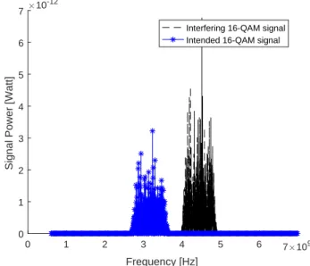
Figure 6: One intended 16-QAM signal and one interfering 16-QAM signal. SNR=15 dB, SIR=12 dB.

simulations. In the simulations the focus was on the last 100 meters at IoT network. There was a total of N devices, which were uniformly and independently deployed in a 2-dimensional circular plane with plane radius R. This deployment results in a 2-D Poisson point distribution of devices. After the network was formed the devices were assumed to be static. The noise was additive white Gaussian noise (AWGN). The signals and the noise were assumed to be uncorrelated. Here, 16-quadrature amplitude modulation (QAM) signal that transmits 4 bits per symbol was used. It is one of the modulation types used in LTE. There were 1024 samples and fast Fourier transformation (FFT) was used. In the simulations, IS and detection were performed at the same time. IS was performed using one threshold Tm = 6.9, as detection was performed

using two LAD thresholds Tu = 9.21 and Tl = 2.3. SNR is

the ratio of intended signal energy to noise power, as signal-to-interference ratio (SIR) is the ratio of intended signal energy to interfering signal energy.

The first situation is like (3), i.e., there is PU-SU

in-0 1 2 3 4 5 6 7 Frequency [Hz] 109 0 1 2 3 4 5 6 7

Signal power [Watt]

10-12

Detected signal

Suppressed signal

Interfering 16-QAM signal Intended 16-QAM signal

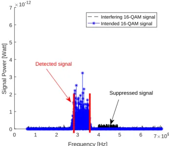
Figure 7: One intended 16-QAM signal and one interfering 16-QAM signal. After interference suppression and detection. SNR=15 dB, SIR=12 dB. 0 1 2 3 4 5 6 _{7 10}9 Frequency [Hz] 0 1 2 3 4 5 6 7

Signal Power [Watt]

10-12

Interfering 16-QAM signal Intended 16-QAM signal

Figure 8: One intended 16-QAM signal and one interfering 16-QAM signal. SNR=12 dB, SIR=15 dB.

terference (Figure 5). Thus, the received signal is of form r2(n) = s(n) + i2(n) + η, where s(n) and i2(n) are both

16-QAM signals. Now, s(n) is intended signal (red arrow) as i2(n) is interfering signal from PU (blue arrow). Their

bandwidth covers about 30% of the total bandwidth. In Fig-ure 6, SNR=15 dB and SIR=12 dB, so intended signal is stronger than interfering signal. Figure 7 shows the situation after interference suppression and signal detection. In Figure 8, SNR=12 dB and SIR=15 dB more, so intended signal is weaker than interfering signal. The situation after signal detection and IS is illustrated in Figure 9. It can be said that both the methods perform well.

Next, r4(n) = s(n) +P 3

j=2ij(n) + η like in (5). Now

0 1 2 3 4 5 6 _{7 10}9 Frequency [Hz] 0 1 2 3 4 5 6 7

Signal Power [Watt]

10-12

Suppressed signal Detected signal

Interfering 16-QAM signal Intended 16-QAM signal

Figure 9: One intended 16-QAM signal and one interfering 16-QAM signal. After interference suppression and detection. SNR=12 dB, SIR=15 dB.

Figure 10: Received signals at receiver. Intended signal, PU-SU and PU-SU-PU-SU interference, T=time and f=frequency.

there are two suppressed signals: one is from PU and one is from other SU so there is both PU-SU and SU-SU interference (Figure 10). Now, s(n) is intended signal (red arrow), i2(n)

is interfering signal from PU (blue arrow), and i3(n) is

inter-fering signal from other SU (green arrow). Their bandwidth covers about 45% of the total bandwidth. In Figure 11, all the thresholds Tu, Tland Tmare presented. As the intended signal

is detected using theresholds Tu and Tl, the IS is performed

using threshold Tm. As can be seen, all the signals are found

and both the interfering signals are suppressed. B. Measurements

The IS performance of the FCME method against RNB signals was studied using real-world wireless data. The re-sults are based on real-life measurements. Measurements were performed using spectrum analyzer Agilent E4446 [45] (Fig-ure 12). Three types of signals were studied, namely the LTE uplink, LTE downlink, and WLAN signals. All those signals are commonly used wireless signals. Both LTE1800

0 1 2 3 4 5 6 Frequency [Hz] 109 0 0.5 1 1.5 2 2.5 3 3.5 4

Signal power [Watt]

10-12 Upper threshold T_u Lower threshold T l Middle threshold T m Detected signal Suppressed signals

Interfering 16-QAM signal Intended 16-QAM signal

Figure 11: One intended 16-QAM signal and two interfering 16-QAM signals. Interference suppression (Tm) and detection

(Tu and Tl) thresholds. SNR=15 dB, SIR=12 dB.

Figure 12: Agilent E4446. LTE1800 network downlink signals.

network frequencies and WLAN signals were measured at the University of Oulu, Finland. IS was performed using the FCME method with threshold parameter 4.6, i.e., desired false alarm rate PF A,DES= 1% = 0.01 [20].

LTE1800 network operates at 2 × 75 MHz band so that uplink is on 1.710 − 1.785 GHz and downlink is on 1.805 − 1.880 GHz [46]. LTE downlink uses OFDM signal as uplink uses SC-FDMA. LTE assumes a small nominal guard band (10% of the band, excluding 1.4 MHz case).

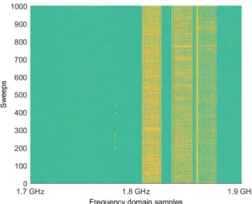
One measurement at 1.7 − 1.9 GHz containing 1000 time domain sweeps and 1601 frequency domain points is seen in Figure 13. Therein, yellow means strong signal power (=signal) as green means weaker signal power (=noise). Therein, only downlink signaling is present. Downlink signals have larger interference distance than uplink signals. Interfering signals cover about 30% of the studied bandwidth. In Figure 14, situation after the FCME IS is presented. Therein, yellow means strong signal power as white means no signal power. It can be seen that the signals (white) have been suppressed and the noise is now dominant (yellow). On uplink signal frequencies where no signals are present (600 first frequency

Figure 13: LTE1800 network frequencies. Spectrogram of downlink signals present.

Figure 14: LTE1800 network frequencies. Spectrogram of suppressed downlink signals. The FCME method was used.

domain samples), average noise value is −99 dBm before and after IS.

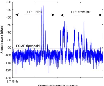
In Figure 15, first line (sweep) of the previous case is presented more closely. The FCME thresholds after two cases are presented. In the first case, the FCME is calculated using frequencies 1.8 − 1.9 GHz (downlink). Interfering signals cover about 60% of the studied bandwidth. The threshold is −89 dBm (upper line). In the second case, the threshold is calculated using both uplink and downlink frequencies 1.7−1.9 GHz when there is no uplink signals (like case in Figure 13), i.e., SU is so far away from PU that only downlink signals are present. Interfering signals cover about 30% of the studied bandwidth. In that case, the threshold is −91 dBm (lower

1.8 GHz 1.85 GHz 1.9 GHz −130 −120 −110 −100 −90 −80 −70 −60

Frequency domain samples

Signal power [dBm]

FCME threhsold

Figure 15: IS using the FCME method for LTE downlink sig-nals. Upper threshold when the FCME calculated on 1.8 − 1.9 GHz, lower threshold (dashed line) when the FCME calculated on 1.7 − 1.9 GHz.

Figure 16: LTE1800 network frequencies. Uplink and down-link signals present.

dashed threshold). It can be noticed that when the studied bandwidth is doubled and this extra band contains only noise, we get 2 dB gain.

Next, both uplink and downlink signals are present. There were 2001 frequency domain points and 1000 time sweeps. Figure 16 presents one measurement at 1.7 − 1.9 GHz. Both uplink and downlink signals are present. In Figure 17, one snapshot when both uplink and downlink signals are present is presented. Therein, both signals are suppressed.

In the WLAN measurements, 2.4−2.5 GHz frequency area was used. There were 1000 sweeps and 1201 frequency domain data points. In Figure 18, one snapshot is presented when there is a WLAN signal present and the FCME algorithm is used to perform IS. As can be seen, the WLAN signal is found.

1.7 GHz

Frequency domain samples

-130 -120 -110 -100 -90 -80 -70 -60 -50 -40 -30 Signal power [dBm] FCME threshold

LTE uplink LTE downlink

Figure 17: LTE1800 network frequencies. Uplink and down-link signals present. IS using the FCME method.

2.4 GHz 2.45 GHz 2.5 GHz −125 −120 −115 −110 −105 −100 −95 −90 −85 −80 −75

Frequency domain samples

Signal power [dBm]

FCME threshold

Figure 18: IS using the FCME method at frequencies 2.4 − 2.5 GHz where WLAN signals exist. Threshold is −90 dBm.

Next, the desired false alarm rate (PF A,DES) values are

compared to the achieved false alarm rate (PF A) values in

the noise-only case. Figure 19 presents one situation when there is only noise present. According to the definition of the FCME method, threshold parameter 4.6 means that 1% of the samples is above the threshold when there is only noise present. Here, there are 1201 samples so PF A,DES= 1% = 12

samples. In Figure 19, 12 samples are over the threshold, so PF A,DES = PF A. We had 896 measurement sweeps in the

noise-only case at WLAN frequencies. Therein, minimum 1 sample and maximum 19 samples were over the threshold as the mean was 10 samples and median value was 9 samples. Those were close of required 12 samples. Note that the definition has been made for pure AWGN noise.

2.4 GHz 2.45 GHz 2.5 GHz −125 −120 −115 −110 −105 −100 −95 −90 −85 −80 −75

Frequency domain samples

Signal power [dBm]

FCME threshold

Figure 19: IS using the FCME method at frequencies 2.4 − 2.5 GHz where are no signals present. Threshold is −91 dBm. 1% = 12 samples are above the threshold, as expected.

VII. CONCLUSION

In this paper, the performance of the forward consecutive mean excision (FCME) interference suppression method was studied against relatively narrowband interfering signals exist-ing in the novel cognitive radio networks. The focus was on interference suppression in secondary user receiver suffering interfering signals caused by primary and other secondary users. In addition, the extension of the FCME method called the localization algorithm based on double-thresholding (LAD) method that uses three thresholds was proposed to be used for both interference suppression and intended signal detection. LTE simulations confirmed the performance of the extended LAD method that uses three thresholds. Real-world LTE and WLAN measurements were performed in order to verify the performance of the FCME method. It was noted that the extended LAD method that uses three thresholds can be used for detecting and suppressing LTE signals, and the FCME method is able to suppress LTE OFDM and SC-FDMA signals as well as WLAN signals. Our future work includes statistical analysis, more detected and suppressed signals, as well as comparisons to other methods.

ACKNOWLEDGMENT

The research of Johanna Vartiainen was funded by the Academy of Finland.

REFERENCES

[1] J. Vartiainen and R. Vuohtoniemi, “LTE and WLAN interference suppression in CR applications,” in Proc. The Sixth International Con-ference on Advances in Cognitive Radio (COCORA), Lisbon, Portugal, Feb. 2016, pp. 33–38.

[2] J. Mitola III and G. Q. M. Jr., “Cognitive radio: making software radios more personal,” IEEE Pers. Commun., vol. 6, no. 4, 1999, pp. 13–18. [3] S. Haykin, “Cognitive radio: Brain-empowered wireless communica-tions,” IEEE J. Select. Areas Commun., vol. 23, no. 2, Feb. 2005, pp. 201–220.

[4] V. Chakravarthy, A. Shaw, M. Temple, and J. Stephens, “Cognitive radio - an adaptive waveform with spectral sharing capability,” in IEEE Wireless Commun. and Networking Conf., New Orleans, LA, USA, Mar.13–17 2005, pp. 724–729.

[5] S. N. Shankar, C. Cordeiro, and K. Challapali, “Spectrum agile radios: Utilization and sensing architectures,” in IEEE Int. Symposium on Dy-namic Spectrum Access Networks (DySpAN) 2005, vol. 1, Baltimore, USA, Nov. 2005, pp. 160–169.

[6] T. Yucek and H. Arslan, “A survey of spectrum sensing algorithms for cognitive radio applications,” IEEE Commun. Surveys and Tutorials, vol. 11, no. 1, 2009, pp. 116–130.

[7] J. Mitola III, “Cognitive radio architecture evolution,” IEEE Proceed-ings, vol. 97, no. 4, 2009, pp. 626–641.

[8] S. Haykin, D. J. Thomson, and J. H. Reed, “Spectrum sensing for cog-nitive radio - the utility of the multitaper method and cyclostationarity for sensing the radio spectrum, including the digital tv spectrum, is studied theoretically and experimentally,” Proc. of the IEEE, vol. 97, no. 5, May 2009, pp. 849–877.

[9] 3GPP, “The mobile broadband standard,” (2013), http://www.3gpp.org [retrieved: May, 2017].

[10] K. Ashton, “That ’internet of things’ thing,” RFID Journal, June 2009, http://www.rfidjournal.com/articles/view?4986 [retrieved: May, 2017]. [11] J. Voas, “Networks of ’things’,” NIST Special Publication 800-183,

July 2016. http://dx.doi.org/10.6028/NIST. SP.800-183 [retrieved: May, 2017].

[12] O.-C. Iacoboaiea, B. Sayrac, S. B. Jemaa, and P. Bianchi, “SON coordi-nation in heterogenous networks: A reinforcement learning framework,” IEEE Trans. Wirel. Commun., vol. 15, no. 9, 2016, pp. 5835–5847. [13] R. F. Shigueta, M. Fonseca, A. C. Viana, A. Ziviani, and A. Munaretto,

“A strategy for opportunistic cognitive channel allocation in wireless internet of things,” in IFIP Wireless Days, Rio de Janeiro, Brazil, Nov 2014.

[14] A. Alja and A. H. Aghvami, “Cognitive machine-to-machine communi-cations for internet-of-things: A protocol stack perspective,” IEEE IoT Journal, vol. 2, no. 2, 2016, pp. 103–112.

[15] A. Nordrum, “Popular internet of things forecast of 50 billion devices by 2020 is outdated,” in IEEE Spectrum, Aug. 2016, http://spectrum.ieee.org/tech-talk/telecom/internet/popular-internet-of-things-forecast-of-50-billion-devices-by-2020-is-outdated [retrieved: May, 2017].

[16] Z. Chen, “Interference modelling and management for cogni-tive radio networks,” Ph.D. dissertation, Doctoral Thesis (sub-mitted), Apr. 2011, http://www.ros.hw.ac.uk/bitstream/10399/2421/1/ ChenZ 0511 eps.pdf [retrieved: May, 2017].

[17] K. Nishimori, H. Yomo, and P. Popovski, “Distributed interference cancellation for cognitive radios using periodic signals of the primary system,” IEEE Trans. Wirel. Commun., vol. 10, no. 9, 2011, pp. 2971 – 2981.

[18] J. Peha, “Spectrum sharing in the gray space,” Telecommunications Policy Journal, vol. 37, no. 2-3, 2013, pp. 167–177.

[19] H. Saarnisaari, P. Henttu, and M. Juntti, “Iterative multidimensional impulse detectors for communications based on the classical diagnostic methods,” IEEE Trans. Commun., vol. 53, no. 3, Mar. 2005, pp. 395– 398.

[20] J. Vartiainen, “Concentrated signal extraction using consecutive mean excision algorithms,” Ph.D. dissertation, Acta Univ Oul Technica C 368. Faculty of Technology, University of Oulu, Finland, Nov. 2010, http: //jultika.oulu.fi/Record/isbn978-951-42-6349-1 [retrieved: May, 2017]. [21] J. Vartiainen, J. J. Lehtom¨aki, and H. Saarnisaari, “Double-threshold based narrowband signal extraction,” in Proc. IEEE Veh. Technol. Conf. (VTC) 2005, Stockholm, Sweden, May/June 2005, pp. 1288–1292. [22] J. Vartiainen, J. J. Lehtom¨aki, H. Saarnisaari, and M. Juntti,

“Two-dimensional signal localization algorithm for spectrum sensing,” IEICE Trans. Commun., vol. E93-B, no. 11, Nov. 2010, pp. 3129–3136. [23] J. A. Stankovic, “Research directions for the internet of things,” IEEE

Int. of Things Journal, vol. 1, no. 1, Feb. 2014, pp. 3–9.

[24] A. H. Ngu, M. Gutierrez, V. Metsis, S. Nepal, and Q. Z. Sheng, “IoT middleware: A survey on issues and enabling technologies,” IEEE Int. of Things Journal, vol. 4, no. 1, Feb. 2017, pp. 1–20.

[25] P. Karunakaran, T. Wagner, A. Scherb, and W. Gerstacker, “Sensing for spectrum sharing in cognitive LTE-A cellular networks,” cornell Uni-versity Library. http://arxiv.org/abs/1401.8226 [retrieved: May, 2017].

[26] L. Zhang, L. Yang, and T. Yang, “Cognitive interference management for LTE-A femtocells with distributed carrier selection,” in Proc. IEEE Veh. Technol. Conf. (VTC) Fall, 2010, pp. 1–5.

[27] V. Osa, C. Hearranz, J. F. Monserrat, and X. Gelabert, “Implementing opportunistic spectrum access in LTE-advanced,” EURASIP Journal on Wireless Communications and Networking, vol. 99, 2012, pp. 1–17. [28] Q. Wu et al., “Cognitive internet of things: A new paradigm beyond

connection,” IEEE Journal of Internet of Things, vol. 1, no. 2, 2014, pp. 1–15, [retrieved: May, 2017].

[29] J. Tervonen, K.Mikhaylov, S. Pieska, J. Jamsa, and M.Heikkila, “Cogni-tive internet-of-things solutions enabled by wireless sensor and actuator networks,” in IEEE Conf. on Cognitive Infocommun. (CogInfoCom), 2014, pp. 97–102.

[30] F. Xia, L. T. Yang, L. Wang, and A. Vine, “Internet of things,” Int. Journal of Commun. Systems, vol. 25, 2012, pp. 1101–1102. [31] LoRa, http://lora-alliance.org/ [retrieved: May, 2017]. [32] Neul, www.neul.com [retrieved: May, 2017]. [33] SigFox, www.sigfox.com [retrieved: May, 2017].

[34] Nokia, “LTE M2M - optimizing LTE for the internet of things,” in White paper, 2014, http://networks.nokia.com/file/34496/lte-m-optimizing-lte-for-the-internet-of-things [retrieved: May, 2017].

[35] J. Gozalvez, “New 3GPP standarf for IoT,” IEEE Vehicular Technology Magazine, vol. 11, no. 1, Mar. 2016, pp. 14–20.

[36] 3GPP16, “Standardization of NB-IOT completed,” (2016), http://www.3gpp.org/news-events/3gpp-news [retrieved: May, 2017]. [37] Z. Feng and Y. Xu, “Cognitive TD-LTE system operating

in TV white space in china,” ITU-R WP 5A, Geneva, Switzerland, (2013), http://studylib.net/doc/13258156/ cognitive-td-lte-system-operating-in-tv-white-space-in-china [retrieved: May, 2017].

[38] J. Mitra and L. Lampe, “Sensing and suppression of impulsive interfer-ence,” in Canadian Conference on Electrical and Computer Engineering (CCECE), Canada, May 2009, pp. 219–224.

[39] Y. Ma, D. I. Kim, and Z. Wu, “Optimization of OFDMA-based cellular cognitive radio networks,” IEEE Trans. on Commun., vol. 58, no. 8, 2010, pp. 2265–2276.

[40] J. Andrews, “Interference cancelation for cellular systems: a contempo-rary overview,” IEEE Wireless Comm., vol. 12, no. 2, Apr. 2005, pp. 19–29.

[41] X. Hong, Z. Chen, C.-X. Wang, S. A. Vorobyov, and J. S. Thompson, “Cognitive radio networks - interference cancelation and management techniques,” IEEE Veh. Technol. Magazine, Dec. 2009, pp. 76–84. [42] L. B. Milstein and P. K. Das, “An analysis of a real-time transform

domain filtering digital communication system - part I: Narrowband interference rejection using eral-time Fourier transforms,” IEEE Trans. Commun., vol. 28, 1980, pp. 816–824.

[43] J. Vartiainen, J. J. Lehtom¨aki, H. Saarnisaari, and M. Juntti, “Analysis of the consecutive mean excision algorithms,” J. Elect. Comp. Eng., 2011, pp. 1–13.

[44] J. Vartiainen, H. Sarvanko, J. Lehtom¨aki, M. Juntti, and M. Latva-aho, “Spectrum sensing with LAD based methods,” in Proc. IEEE Int. Symp. Pers., Indoor, Mobile Radio Commun. (PIMRC), Athens, Greece, Aug. 2007, pp. 1–5.

[45] Agilent, http://www.agilent.com [retrieved: May, 2017].

[46] Nokia Siemens Networks, “Introducing LTE with max-imum reuse of GSM assets,” in White paper, 2011, http://www.gsma.com/spectrum/introducing-lte-with-maximum-reuse-of-gsm-asset/ [retrieved: May, 2017].

Impact of Analytics and Meta-learning on Estimating Geomagnetic Storms

A Two-stage Framework for Prediction

Taylor K. Larkin

and Denise J. McManus

Information Systems, Statistics, and Management Science Culverhouse College of Commerce

The University of Alabama Tuscaloosa, AL 35487-0226

Email: tklarkin@crimson.ua.edu1_{, dmcmanus@cba.ua.edu}2

Abstract—Cataclysmic damage to telecommunication infrastruc-tures, from power grids to satellites, is a global concern. Nat-ural disasters, such as hurricanes, tsunamis, floods, mud slides, and tornadoes have impacted telecommunication services while costing millions of dollars in damages and loss of business. Geomagnetic storms, specifically coronal mass ejections, have the same risk of imposing catastrophic devastation as other natural disasters. With increases in data availability, accurate predictions can be made using sophisticated ensemble modeling schemes. In this work, one such scheme, referred to as stacked generalization, is used to predict a geomagnetic storm index value associated with 2,811 coronal mass ejection events that occurred between 1996 and 2014. To increase lead time, two rounds (stages) of stacked generalization using data relevant to a coronal mass ejection’s life span are executed. Results show that for this dataset, stacked generalization performs significantly better than using a single model in both stages for the most important error metrics. In addition, overall variable importance scores for each predictor variable can be calculated from this ensemble strategy. Utilizing these importance scores can help aid telecommunication researchers in studying the significant drivers of geomagnetic storms while also maintaining predictive accuracy.

Keywords–ensemble modeling; space weather; quantile regres-sion; stacked generalization; telecommunications.

I. INTRODUCTION

Predicting geomagnetic storms is an ever-present problem in today’s society, given the increased emphasis on advanced technologies [1]. These storms are fueled by coronal mass ejections (CMEs), which are colossal bursts of magnetic field and plasma from the Sun as displayed in Figure 1. Typically, a CME travels at speeds between 400 and 1,000 kilometers per second [2] resulting in an arrival time of approximately one to four days [3]; however, they can move as slowly as 100 kilometers per second or as quickly as 3,000 kilometers per second (or around 6.7 million miles per hour) [4]. These phenomena can contain a mass of solar material exceeding 1013 kilograms (or approximately 22 trillion pounds) [5] and can explode with the force of a billion hydrogen bombs [6]. Naturally, CME events are often associated with solar activity such as sunspots [4]. During the solar minimum of the 11 year solar cycle (the period of time where the Sun has fewer sunspots and, hence, weaker magnetic fields), CME events occur about once a day. During a solar maximum, this daily estimate increases to four or five. One plausible theory for these incidents taking place involves the Sun needing to release energy. As more sunspots develop, more coronal magnetic field structures become entangled; therefore, more energy is

required to control the volatility and convolution. Once the energy surpasses a certain level, it becomes beneficial for the Sun to release these complex magnetic structures [2].

When this force approaches Earth, it collides with the magnetosphere. The magnetosphere is the area encompassing Earth’s magnetic field and serves as the line of defense against solar winds. The National Oceanic and Atmospheric Admin-istration (NOAA) describes this event as “the appearance of water flowing around a rock in a stream” [7] as shown in Figure 2.

Figure 1. LASCO coronagraph images [4], courtesy of the NASA/ESA SOHO mission.

Figure 2. Rendering of Earth’s magnetosphere interacting with the solar wind from the Sun [8], courtesy of the NASA.

After the solar winds compress Earth’s magnetic field on the day side (the side facing the Sun), they travel along the elongated magnetosphere into Earth’s dark side (the side

opposite of the Sun). The electrons are accelerated and ener-gized in the tails of the magnetosphere, filtering down to the Polar Regions and clashing with atmospheric gases causing geomagnetic storms. This energy transfer emits the brilliance known as the Aurora Borealis, or Northern Lights, and the Aurora Australis, or Southern Lights, which can be seen near the respective poles.

While mainly responsible for the illustrious Northern Lights, geomagnetic storms have the potential to cause cata-clysmic damage to Earth. Normally, the magnetic field is able to deflect most of the incoming plasma particles from the Sun. However, when a CME contains a strong southward-directed magnetic field component (Bz), energy is transferred from

the CME’s magnetic field to Earth’s through a process called magnetic reconnection [9][10][11] (as cited in [12]). Magnetic reconnection leads to an injection of plasma particles in Earth’s geomagnetic field and a reduction of the magnetosphere to-wards the equator [2]. Consequently, more energy is amassed in the upper atmosphere, particularly at the poles. Moreover, this energy is impressed upon power transformers causing an acute over-saturation and inducing black-outs via geomag-netically induced currents (GICs) [13]. Some other residuals of this over-accumulation of energy include the corrosion of pipelines, deteriorations of radio and GPS communications, radiation hazards in higher latitudes, damages to spacecrafts, and deficiencies in solar arrays [14]. These ramifications pose a significant threat to global telecommunications and electri-cal power infrastructures as CMEs continue to be launched towards Earth [15] and remain the primary source of major geomagnetic disturbances [16][17][18] (as cited in [19]). From a business perspective, risk factor mitigation is an absolute necessity within the global business environment [20]. This can be accomplished using advanced analytical techniques on data collected about these phenomena.

The subsequent sections of this work read as follows. Sec-tion II introduces previous studies on predicting geomagnetic storms. Section III provides detail about the basics of the methodology used, the dataset studied, and the experimental strategy. Section IV displays and discusses the results as well as postulates areas for future work. Section V concludes with a summary.

II. LITERATUREREVIEW

A. Predicting Dangerous CMEs

CMEs present an ever-increasing threat to Earth as society becomes more dependent on technology, such as satellites and telecommunication operations. Nevertheless, because of this increase in technology, more data has been collected about these acts and the solar wind condition in general. This, in turn, has allowed for empirical models to be developed. Burton, McPherron, and Russell [21] presented an algorithm to predict the disturbance storm time index (DST) value [22] based on solar wind and interplanetary magnetic field parameters. The DST value is a popular metric to assess geomagnetic activity. Expressed in nanoteslas (nT) and recorded every hour from observatories around the world, it measures the depression of the equatorial geomagnetic field, or horizontal component of the magnetic field; thus, the smaller the value of the DST, the more significant the disturbance of the magnetic field [2]. Many researchers have used this information for building forecasting models to predict geomagnetic storms [23][24].

However, many of these systems only use in-situ data, or data that can only be measured close to Earth. To improve prediction, studies have included data gathered at the onset of a CME and the near-Earth interplanetary information (IPI) regarding the solar wind condition as the CME approaches Earth [25][26][27]. These have ranged from using logistic regression [26] to neural networks [28] to make predictions based on this combination of data. Further improvements have been made by using multi-step frameworks. To narrow the scope, this work will focus on reviewing two recent two-step procedures that predict geomagnetic storms using both near-Earth IPI and CME properties taken near the Sun.

Valach, Bochn´ıˇcek, Hejda, and Revallo [29] reinforced one of the primary issues facing geomagnetic storm prediction: the inability to estimate the orientation of the interplanetary magnetic field from an incoming CME more than a few hours out. It is well-known that one of the largest predictor variables is the magnitude of the aforementioned magnetic field component Bz [21][26][2]; however, this is difficult

to predict prior to reaching the L1 Lagrangian point (the position close to Earth where much of the IPI is collected) due to complexities in a CME’s magnetic topology [30]. Hence, under the assumption that the direction of the magnetic field component is unpredictable, the authors first study the behavior of Bz for 2,882 days between 1997 to 2007 before

implementing any predictive construct. Based on their analysis, they determined that for the majority of the days with a high-level of geomagnetic activity, Bz was negative for at least

16 hours during the course of the day (behavior exhibited by roughly 31% of the days studied). Then, after building a neural network using these observations, they forecasted the daily level of geomagnetic activity with initial CME and solar X-ray information. The benefits to their approach are that the predictions are timely (absence of IPI in the second step enable forecasts at least a day out) and are well-suited for the strongest of storms (since the training observations are composed of days where Bz is negative for more than 16 hours). However,

as noted by the authors, it does not do as well differentiating moderate and weak geomagnetic storms. In addition, the time scale of the prediction is in days, which is not as granular as hours.

Kim, Moon, Gopalswamy, Park, and Kim [27] argued that only using information based on urgent warning IPI for pre-diction does not provide a practical lead time for preparations to be made on Earth, even though the forecasts are more accurate. At the same time, strictly employing initial CME data becomes frivolous as each CME experiences changes in composition as they propagate through the interplanetary medium, thereby, making prediction difficult. Therefore, the authors constructed a two-step forecasting system using both urgent warning IPI and initial CME data. At the first stage, they applied multiple linear regression models to predict the strength of geomagnetic activity for northward and southward events at the onset of a CME using its location, speed, and direction parameter (estimated from the magnetic orientation angle of the related active region on the Sun). The estimation of the direction (north or south) is based on the assumption that these rarely deviate from that of the associated active region [31]. Next, they administered a set of rules based on the IPI to update the forecast and classify the impending CME as causing a moderate or intense storm. This method contributes