The Subprime Crisis Effects in
Leverage Mechanisms
Dissertation submitted in partial fulfilment of requirements for the Master
of Science in Finance, at the Universidade Católica Portuguesa
Dissertation written under the supervision of
Professor Diana Bonfim
Afonso Pereira
152418016
Leverage Mechanisms
Abstract
This dissertation documents a thorough investigation about the US nonfinancial firms’ capital structure. It extends the findings of Lemmon et.al (2008) that leverage ratios are characterized by both a permanent and a transitory feature to a more recent timespan including the subprime crisis years and its aftermath. The first means that leverage ratios are driven by an unobserved time-invariant factor that generates remarkably stable capital structures. The latter suggests that there is mean reversion in leverage ratios. In other words, high (low) levered firms tend to converge toward more moderate levels of leverage over time. These features are largely unexplained by previously identified determinants and they are also robust to firm exit or IPO processes. Further, the permanent element persists whether managers are more concerned with short- or long-term equilibriums on leverage determinants. It is also examined the relation between the firms’ net issuance activity and leverage with the results providing a strong evidence that it is an active management behaviour toward desired leverage ratios that is behind the transitory mechanism of leverage. Additionally, this analysis reveals that the tendency to issue debt is negatively correlated to firms’ leverage ratios. This dissertation still details the implications of neglecting the permanent component in future empirical specifications attempting to clarify the capital structure heterogeneity.
JEL Codes: G32.
Keywords: leverage ratios, permanent component, transitory component
Afonso Pereira
nos Mecanismos da Dívida
Abstrato
Esta dissertação documenta um estudo aprofundado sobre a estrutura de capitais das empresas americanas não-financeiras. Esta alarga as conclusões de Lemmon et. al (2008), de que os rácios de endividamento são caracterizados por um componente permanente e um transitório, para um horizonte temporal mais recente que inclui os anos da crise do “subprime” e as suas consequências. O primeiro significa que os rácios de endividamento acontecem devido a um fator invariável e inobservável no tempo que gera estruturas de capitais extraordinariamente estáveis. O último sugere que os rácios de envidamento exibem um fenómeno de reversão à média. Ou seja, empresas muito (pouco) endividadas tendem a convergir para níveis mais moderados de endividamento ao longo do tempo. Estes elementos são escassamente explicados pelos fatores de endividamento previamente identificados e são robustos a saídas de empresas ou a processos de oferta pública inicial. Além disso, o elemento permanente perdura quer os gestores sejam mais apreensivos com equilíbrios a curto ou a longo prazo nos determinantes do endividamento. É também estudada a relação entre a atividade de emissão líquida das empresas e o nível de endividamento com os resultados a indicarem que o mecanismo transitório é gerado por um comportamento de gestão ativo em relação aos rácios de endividamento. Esta análise revela igualmente que a tendência de emissão de dívida das empresas está negativamente correlacionada com o seu rácio de endividamento. Esta dissertação detalha ainda as implicações de negligenciar o componente permanente em futuras análises empíricas sobre a heterogeneidade na estrutura de capitais.
Códigos JEL: G32.
Palavras-chave: rácios de endividamento, componente permanente, componente transitório
Afonso Pereira
the Master of Science in Finance at Universidade Católica Portuguesa. First of all, I would like to thank to all the high-quality professors I had during this time for allowing me to develop my knowledge and for increasing my passion for finance. I believe they gave me a strong foundation in this area that enabled this work to become a reality. Nonetheless, I am particularly grateful to my supervisor, Professor Diana Bonfim, for its crucial support and encouragement during all the dissertation process. The strict deadlines and the high level of requirement in the seminars were also fundamental to push me a step forward.
My appreciation also extends to my seminar colleagues. One of the key factors that made me chose the empirical corporation finance dissertation seminar, in addition to the topic and the supervisor, was the fact that it had a maximum of six students, the lowest among all seminars. I believed that this would be a large advantage because this could increase the level of mutual aid. However, my initial expectations were exceeded because more than a united group we become real friends which made it all easier. Therefore, here is my acknowledgement to David Lopes, Filipe Perre, Isaac Silvestre, Joana Gomes and Manuel Cardoso.
Even though I met extraordinary people during my time at Católica, there was people that had a special impact on me. They are Carlos Lopes, the aforementioned David Lopes Francisco Fonseca, José Gouveia and Mariana Pinto. All of them share an impressive sense of humour in any circumstance, and it was due to them that I was always motivated and happy during this stage of my life. Thus, I am very grateful to them and I sincerely wish them as much success as I would wish for myself.
Last but not least, I am indebted to my family and close friends. Specially to my parents for being an inspiration and for providing an unconditional support in all aspects of my life.
1. Introduction ... 1
2. Literature Review ... 4
3. Data ... 7
4. Methodology and Empirical Analysis ... 9
4.1. The Cross-Section Evolution of Leverage... 9
4.2. The Persistent Component of Leverage ... 14
4.2.1. The Impact of Initial Leverage ... 15
4.2.2. The Leverage Variation ... 17
4.2.3. Managers Reactions to Short-Run and Long-Run Fluctuations ... 19
4.2.4. How Far Does the Persistent Component Go? ... 22
4.2.5. The Permanent Component Implications for Future Empirical Studies ... 24
4.3. The Transitory Component of Leverage ... 24
4.3.1. Factors behind the Transitory Component ... 25
4.3.2. Speed of Adjustment ... 27 5. Robustness Checks ... 30 6. Conclusion ... 31 7. Reference List ... 33 8. Appendices ... 36 8.1. Variables Construction ... 36 8.2. Tables... 37 8.3. Figures ... 43
Table 1: Summary Statistics ... 8
Table 2: The Initial Leverage Effect on Actual Leverage ... 16
Table 3: Variance Decompositions ... 19
Table 4: Short-Run versus Long-Run ... 21
Table 5: The Speed of Adjustment ... 28
Table A1: Correlation Matrix ... 37
Table A2: The Initial Leverage Effect on Actual Leverage (Survivors) ... 38
Table A3: Short-Run versus Long-Run (Survivors) ... 39
Table A4: Pooled OLS versus Firm FE ... 40
Table A5: Summary Statistics (Crisis Subsample) ... 40
Table A6: The Initial Leverage Effect on Actual Leverage (Crisis Subsample) ... 41
Table A7: Variance Decompositions (Crisis Subsample) ... 42
List of Figures Figure 1: Average leverage of actual leverage portfolios in event time ... 10
Figure 2: Average leverage of unexpected leverage portfolios in event time ... 13
Figure 3: Average leverage of unexpected leverage portfolios in event time (IPO sample) ... 23
Figure 4: Net security issuance activity in event time ... 26
Figure A1: Average leverage of actual leverage portfolios in event time (exiting firms) ... 43
Figure A2: Average leverage of actual leverage portfolios in event time (logit leverage) ... 44
Figure A3: Average leverage of unexpected leverage portfolios in event time (alternative) .. 45
1 1. Introduction
The heterogeneity of firm’s capital structure has been exhaustively investigated since the Modigliani and Miller (1958) irrelevance proposition. Nonetheless, the thorough study realized in Lemmon et. al (2008) to assess the progress made by well-known empirical works in this field showed that much is yet to explain even after decades of research. One of the referred authors findings is that leverage ratios are characterized by two notable features that remain largely unexplained. The first is that most of variation in leverage ratios is driven by an unobserved permanent component that generates surprisingly stable capital structures, id est, high (low) levered firms tend to remain as such over noticeably large time horizons. The second is that leverage ratios seem to be additionally characterized by a transitory component. That is, firms with relatively high (low) leverage tend to move toward more moderate levels of leverage over time. Furthermore, they demonstrate that neither traditional (Rajan and Zingales, 1995) nor contemporaneous (Frank and Goyal, 2009) determinants demystified considerably the “capital structure puzzle” put forward by Myers (1984). The fundamental question is: Can these findings be extended to a more recent timespan accounting with the subprime crisis and its aftermath? This is the main research question that this dissertation attempts to disentangle.
The empirical analysis begins with the study of the evolution of leverage ratios for the cross-section of firms through an “event-study” framework. On a yearly basis, firms are sorted into quartiles and it is computed the average leverage ratios of these four portfolios (Low, Medium, High and Very High) over the subsequent 20 years, holding their composition constant. Firms are initially sorted based on their actual leverage ratios. Using this sorting procedure, leverage ratios clearly exhibit the permanent and the transitory feature. However, one of its limitations is that it ignores the substantial correlation existent between leverage and certain determinants, namely firm size as showed in Titman and Wessels (1988) and a posteriori confirmed by the correlation matrix of this empirical work. For this reason, firms are then sorted according to the residuals from a regression of leverage on 1-year lagged determinants proven to have high correlation with leverage, with the objective of merely capturing their “pure” leverage. Nevertheless, the discussed leverage components are robust to this and other drawbacks, such as changes in sample composition (e.g., firm exit).
These findings suggest not only that firms future leverage ratios are closely related to their initial leverage ratios but also that the common identified factors capture a lower portion of the leverage variation than expected. However, both miss a quantitative approach. Hence, it is performed a regression to measure the initial leverage importance as well as a variance
2
decomposition to quantify the explanatory power of commonly used determinants. The regression output proves that historical leverage is a powerful determinant of future leverage ratios. More precisely, it is the second most important determinant for book leverage, only outperformed by Industry Median Book Leverage. Regarding the variance decomposition, it presents adjusted R-squares with a range from 17 to 38 percent for cross-sectional regressions of leverage based on previously identified determinants, depending on the specification. Contrariwise, the previous parameter experiences a significant increase to 60% (66%) for book (market) leverage in a regression of leverage on firm fixed effects, which proxy the permanent component. This implies that most of the leverage variation comes from this time-invariant component, as oppose to the commonly used determinants.
The preceding quantitative analyses disregard long-term effects, given that the control variables (i.e., leverage determinants) are only one-period lagged. However, the marked difference between the explanatory power of standard determinants vis-à-vis the firm fixed effects suggests that managers are concerned about their long-run equilibrium levels, rather than their time-series variation. To examine this possibility, it is estimated a distributed lag model of leverage with a lag length of eight periods. Its results show that some factors cause a higher impact in leverage in the short-term while others are more prolific in the long-term, emphasizing the importance of accounting with extensive range lags in empirical specifications. Notwithstanding, determinants still struggle to explain the leverage variation even with a model allowing leverage adjustments to long-run shifts in determinants. For example, a one percent change in the long-run equilibrium level of Industry Median Book Leverage, the most influential determinant in book leverage, causes an average expected change of 6% in leverage, a small fraction in relation to the 21% unconditional standard deviation of book leverage.
Since the importance of the permanent component in leverage for the selected time period is already acknowledged, the goal is now to find whether differences in leverage persist back in time. Consequently, the main sample is restricted to only include firms which have an IPO date in order to form the unexpected leverage portfolios at the time of the IPO. Afterwards, it is performed a methodology to evaluate the leverage evolution which follows a similar reasoning to that behind the starting study to capture the “pure” leverage, id est, based on a sorting process that deals with the correlation between leverage and commonly used determinants, namely firm size, profitability, market-to-book or tangibility. It reveals that a firm’s capital structure is surprisingly resistant to the complex IPO process. It is still observable a distance across portfolios, except between the Low and Medium portfolios, as well as a mean reversion tendency during time (i.e., transitory component), which is not quick enough to
3
impede the portfolios differences of persisting for a long period. More importantly, this analysis illustrates that high (low) levered private remain as such after going public, regardless of the changes in the firm’s control, different information environments or alterations in the access to capital markets occurring during IPO processes.
The existence of this firm-specific effect is of utterly importance for future research works (Rauh and Sofi, 2011) because Pooled OLS regressions, the current workhorses of the empirical capital structure literature, neglect the permanent component. To better understand the implications of this feature for forthcoming researches and check how sensible the previous analyses, conducted through Pooled OLS, are to the specification adopted, two regressions are run. The first uses a Pooled OLS estimation, ignoring firm fixed effects (proxy the permanent component) and serial correlation in the error structure (account with the transitory feature). The second is a firm fixed effect estimation. The leverage factors decline, on average, 94% (79%) for book (market) leverage when we transact to a regression with firm fixed effects. Even though the firm fixed effects remove some of the cross-sectional variation of determinants, this striking difference shows that ignoring the permanent component (i.e., firm fixed effects) or serial correlations in empirical models may lead to biased estimates (Hsiao, 2014).
The methodology then proceeds to the transitory feature. To begin it is examined if this leverage ratios mechanism is product of an active management toward desired leverage ratios or of a more passive behaviour, which is a topic that has attracted strong interest among academics (e.g., Leary and Roberts, 2005, Flannery and Rangan, 2006 and Huang and Ritter, 2009). To distinguish between both hypotheses, it is investigated the correlation between leverage and the net issuance activity. This study concludes that the firm’s tendency to issue debt is negatively correlated with their leverage ratios. Thereby, the mean-reversion effect seems to be driven by an active management of leverage ratios through net debt issues. Next, it is gauged if the active rebalancing is toward time-varying or time-unvarying target leverages. For that, it is computed the speed of adjustment (SOA) using a two-step regression methodology and different specifications. The outcomes show that including time-varying characteristics in the target specification cause marginal changes in the estimated SOA either on Pooled OLS, Firm Fixed Effects or GMM models. This suggests that target leverages are largely time-invariant, contrary to the conclusions of, for example, Hovakimian et. al (2001).
The remainder of this dissertation is organized as follows. Section 2 reviews the literature on capital structure decisions. Section 3 details the data used and the descriptive statistics. Section 4 reports the methodology and empirical findings. Section 5 displays robustness tests. Section 6 concludes. Section 7 (section 8) presents the references (appendices).
4 2. Literature Review
Firms capital structure decisions have been one of the most revisited topics within the realm of corporate finance literature. Modigliani and Miller’s (1958) irrelevance proposition can be deemed as the genesis of this wide debate about the optimal distribution of firm’s liabilities. This theory claims that the total value of a firm is not affected by its choice of capital structure. However, subsequent studies revealed some limitations within this theory. Modigliani and Miller (1963) themselves were one of them. The authors corrected their previous study, explaining that debt tax advantages turned out to be larger than they originally suggested. In fact, this and others market imperfections made this theory only valid in a market under strict conditions, commonly referred in finance as perfect capital markets. Nonetheless, not only tax shields but also other shortcomings of the irrelevance proposition such as agency costs, financial distress costs or information asymmetries were the cornerstones to the first empirical works trying to disassemble the capital structure puzzle.
Traditionally, there are two frameworks to think about capital structure: the pecking order and the static trade-off (Kraus and Litzenberger, 1973). The pecking order theory defends that firms financing choices must rely primarily on internal funds, and that when external financing is needed, firms should always favour debt to equity (Myers, 1984 and Myers and Majluf, 1984). Hence, firm’s leverage is driven by the firm’s net cash flows (Fama and French, 2002). Conversely, the trade-off framework states that maximizing firm value is possible with an optimal debt structure that involves a trade-off between the tax advantages of debt and its related costs (Bradley et. al, 1984). Beyond these two theories, there is another well-known approach. The free cash flow theory (Jensen, 1986), which was conceived for mature firms that are susceptible to overinvest. The underlying idea behind this notion is that very high leverage ratios will increase the firm value when firms operating cash flows significantly exceed its profitable investment opportunities (Myers, 2001).
Conventional theories provided robust insights to the capital structure field (Fama and French, 2005) and they might be considered as good conditional theories (Myers, 2001). Furthermore, they were the foundation to identify numerous determinants that may affect the firm’s debt equity choice such as tangibility, market-to-book, size or profitability (Rajan and Zingales, 1995). However, regressions from traditional models present extremely lows R-squares coefficients, which means that the previously identified determinants have a reduced explanatory power. More recently, this struggle of determinants from traditional models to explain cross-sectional and time-series variation has attracted strong interest among academics.
5
For instance, Lemmon et. al (2008) studied the evolution of leverage for their cross-section of firms. This analysis showed that leverage ratios seem to be characterized by both a transitory and a permanent component. Moreover, these authors also performed a regression of leverage on firm fixed effects that yielded an adjusted R-square of 60%, three times more than traditional regressions. Therefore, we can conclude that most of the total variation in capital structure results from time-invariant factors and it is firm-specific. These results are consistent with the findings in Frank and Goyal (2008). The previous authors show that the aggregate leverage in the U.S has been remarkably stable over time. This may indicate that models that do not include firm fixed effects or serial correlation can lead to omitted variable biases in our results (Arellano, 2003 and Hsiao, 2014), impeding the establishment of causal inferences, given that some firms parameters such as differences in market power or managerial behaviour are difficult to estimate. Notwithstanding, it is necessary further research about which firm-specific characteristics are missing from models (Graham and Leary, 2011). Additionally, the regression on firm fixed effects results also highlight the importance of cross-sectional variation, as opposed to time-series. Regarding the former, most variation seems to be originated from firms within the same industry (Mackay and Philips, 2005).
The transitory component, one of the identified leverage ratios features, can be a consequence of the active management of leverage ratios. Firms convergence towards a target leverage ratio is a topic that has been thoroughly investigated (Leary and Roberts, 2005, Liu, 2005, Flannery and Rangan, 2006, Hovakimian, 2006, Kayhan and Titman, 2007, Strebulaev, 2007, Huang and Ritter, 2009, Antão and Bonfim, 2012). In these empirical works, distinct estimation techniques (OLS regressions, fixed effects, GMM, IV) were used to compute the speed of adjustment. Nevertheless, as Graham and Leary (2011) show, the estimation method used affects the speed of adjustment. Using an OLS approach, Kayhan and Titman (2007) obtain an estimate of 10 percent. In other words, on average, each year a firm is ten percent closer to its optimal leverage ratio. This result is consistent with the findings in Fama and French (2002) that observed a speed of adjustment between 9 and 18 percent. These slow adjustment speed made academics reconsider if firms converge towards a target leverage ratio. In turn, studies accounting for firm effects, such as the ones from Flannery and Rangan (2006) and Lemmon et. al (2008), achieve a considerably higher speed of adjustment (38 and 39 percent, respectively). These results are also robust for Portuguese smaller firms (Antão and Bonfim, 2012). Thus, accounting for time-varying factors appears to measure more accurately the rate that firms adjust toward a target debt to equity ratio, indicating once again that firm fixed effects capture a significant portion of the unexplained capital structure variation.
6
However, this view is not consensual across literature. The presence of adjustment costs (Leary and Roberts, 2005) or market frictions (Strebulaev, 2007), and the issuance of transitory debt obligations by firms to investment opportunities (De Angelo et. al, 2011) are some literature arguments to justify slower adjustment speeds.
All topics addressed on this section have diversified and intensive empirical analysis involved. Notwithstanding, the situation changes when we progress to the permanent component identified in the leverage ratios in Lemmon et. al (2008). Their paper explains that the analysis of this unobserved permanent component requires innovative strategies, namely fixed effects (Bertrand and Schoar, 2003), instrumental variables (Faulkender and Petersen, 2006), natural experiments (Leary, 2009 and Lemmon and Roberts, 2010) or structural estimations (Hennessy and Whited 2005, 2007), due to the limitations of other methods to deal with the observed heterogeneity of capital structures. Moreover, in their study it was also shown that this permanent feature is robust to firm exit and that it persists after the IPO, even with the changes in capital market access or information environment that occur at the time of the IPO. Even though the paper unveiled some empirical difficulties to identify which determinants affect firm’s capital structure, it also narrowed the scope for forthcoming investigations.
This dissertation seeks to test the explanatory power of traditional models and of their correspondent identified factors. But one should have in mind that several subsequent empirical studies widened the range of possible explanations to firm’s capital structure decisions. Two of the most remarkable ones are the market timing theory (Baker and Wurgler, 2002) and the mechanical stock price explanation (Welch, 2004). The first found that firms’ current capital structures are strongly related to their historical market values, whereas the second explains how market leverage ratios vary according to share price fluctuations. Finally, another notable research work is the one from Kisgen (2006). The major finding of this paper was that firms near a credit rating change, whether an upgrade or a downgrade, will on average issue less net debt, relative to the firm's total assets, in comparison with firms which are not. This matter should be studied further, because credit ratings are considered the second most important finance function to determine the appropriate level of debt for companies (Graham and Harvey, 2001).
7 3. Data
The core sample of this study comprises all nonfinancial firm-years observations available in the annual Compustat database between 1980 and 2018.1 Given that the sample
excludes financial firms, SIC codes between 6000 and 6999 were removed. Duplicated observations and firm-years with missing data for book assets were also excluded from the analysis. The items necessary to calculate the variables were extracted in its entirety from the Compustat database. For some analysis it is also required an IPO date. In this case, the data is gathered from Jay Ritter database which provides a more complete information on this parameter. Concerning book and market leverage ratios, only observations that take a value within the closed unit interval are considered. The remaining ratios are trimmed at the upper and lower one-percentiles, in order to mitigate the effect of outliers and eliminate errors from the data.2 Regarding computations involving any relevant variable, firm-years with missing data
for that variable were deleted. The construction of all variables used in this dissertation is detailed in the Appendix. Furthermore, for most of the subsequent analyses it is additionally examined a subsample just including firms having at least 20 years of nonmissing data on book leverage, even if these years are not consecutive, as a robustness check, due to the potential for survivorship bias of the primary sample. It is denominated as “Survivors”, because it requires a minimum of 20 years of existence.
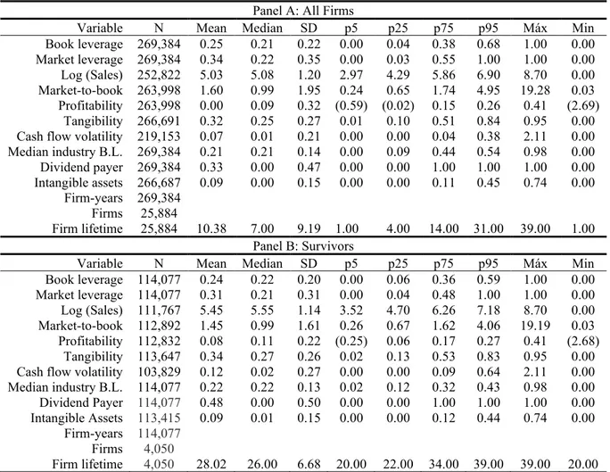
Table 1, Panel A reports the summary statistics for the entire sample. After applying the abovementioned restrictions, it ends up with a total of 269,384 firm-years that correspond to 25,884 firms. The average firm’s lifetime is 10.38 years. Table 1, Panel B details the descriptive statistics for the subsample Survivors. It includes an aggregate of 4,050 firms that cover 114,077 firm-years, after the data filters. As expected, due to the requirement of only including firms with no less than 20 years of existence, the average firm’s lifetime is substantially higher in relation to the whole sample, 28.02 years. Most of the results in Table 1 are consistent with Lemmon et. al (2008) findings. Survivor’s firms are larger and more profitable, have fewer growth opportunities (as the lower Market-to-book ratio reveals), have a higher tangibility ratio and tend to pay dividends more frequently. These authors also found that Survivors normally
1This time horizon covers most of the years used by Lemmon et. al (2008), and simultaneously checks if their findings still hold the financial crisis and its aftermath are considered. The impact of the financial crisis on firms’ capital structures is significant. Fosberg (2012) shows that the amount of leverage was considerably higher on the pre-crisis and crisis period, especially in market value terms.
2It is followed the same method to deal with errors outliers that Lemmon et. al (2008) applied, in order to facilitate results comparisons.
8
have more leverage, especially in market value terms. The book and the market leverage are slightly lower for Survivors in this time period. However, the Industry Median Book Leverage is higher for Survivors as in their study. Specifically, it has a value of 22 percent for Survivors and 21 percent for primary sample. Thus, on the topic of leverage, the results for this time horizon are not completely in line with the ones of the aforementioned authors.
Table 1 Summary Statistics
The table comprises the following data: number of observations, mean, median, the standard deviation, some percentiles (5th, 25th, 75th and 95th), and the maximum and minimum for each
variable. Panel A presents the descriptive statistics for the primary sample. Panel B summarizes the statistics for the subsample constituted by firms having at least 20 years of nonmissing data in book leverage. The construction of the variables is detailed in the Appendix.
Panel A: All Firms
Variable N Mean Median SD p5 p25 p75 p95 Máx Min Book leverage 269,384 0.25 0.21 0.22 0.00 0.04 0.38 0.68 1.00 0.00 Market leverage 269,384 0.34 0.22 0.35 0.00 0.03 0.55 1.00 1.00 0.00 Log (Sales) 252,822 5.03 5.08 1.20 2.97 4.29 5.86 6.90 8.70 0.00 Market-to-book 263,998 1.60 0.99 1.95 0.24 0.65 1.74 4.95 19.28 0.03 Profitability 263,998 0.00 0.09 0.32 (0.59) (0.02) 0.15 0.26 0.41 (2.69) Tangibility 266,691 0.32 0.25 0.27 0.01 0.10 0.51 0.84 0.95 0.00 Cash flow volatility 219,153 0.07 0.01 0.21 0.00 0.00 0.04 0.38 2.11 0.00 Median industry B.L. 269,384 0.21 0.21 0.14 0.00 0.09 0.44 0.54 0.98 0.00 Dividend payer 269,384 0.33 0.00 0.47 0.00 0.00 1.00 1.00 1.00 0.00 Intangible assets 266,687 0.09 0.00 0.15 0.00 0.00 0.11 0.45 0.74 0.00 Firm-years 269,384 Firms 25,884 Firm lifetime 25,884 10.38 7.00 9.19 1.00 4.00 14.00 31.00 39.00 1.00 Panel B: Survivors
Variable N Mean Median SD p5 p25 p75 p95 Máx Min Book leverage 114,077 0.24 0.22 0.20 0.00 0.06 0.36 0.59 1.00 0.00 Market leverage 114,077 0.31 0.21 0.31 0.00 0.04 0.48 1.00 1.00 0.00 Log (Sales) 111,767 5.45 5.55 1.14 3.52 4.70 6.26 7.18 8.70 0.00 Market-to-book 112,892 1.45 0.99 1.61 0.26 0.67 1.62 4.06 19.19 0.03 Profitability 112,832 0.08 0.11 0.22 (0.25) 0.06 0.17 0.27 0.41 (2.68) Tangibility 113,647 0.34 0.27 0.26 0.02 0.13 0.53 0.83 0.95 0.00 Cash flow volatility 103,829 0.12 0.02 0.27 0.00 0.00 0.09 0.64 2.11 0.00 Median industry B.L. 114,077 0.22 0.22 0.13 0.02 0.12 0.32 0.43 0.98 0.00 Dividend Payer 114,077 0.48 0.00 0.50 0.00 0.00 1.00 1.00 1.00 0.00 Intangible Assets 113,415 0.09 0.01 0.15 0.00 0.00 0.12 0.44 0.74 0.00 Firm-years 114,077 Firms 4,050 Firm lifetime 4,050 28.02 26.00 6.68 20.00 22.00 34.00 39.00 39.00 20.00
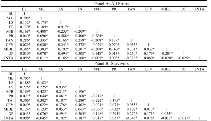
Table A1, in Appendix, reports the correlation matrix for the variables considered in this dissertation. Panel A displays the correlation coefficients using the main sample. In turn, Panel B shows the correlation coefficients for the subsample Survivors. All variable correlations in both samples are statistically significant at a 5 percent level. Firm Size was added to the matrix in order to examine if the variable Log (Sales) is a good proxy for size, given that the latter will be used frequently as a size measure. These two variables reveal a very high
9
correlation coefficient (0.917 for all firms and 0.935 for Survivors), significant at a 5% level. Therefore, Log (Sales) is a valid proxy for size. Moreover, Firm Size is positively and significantly correlated with leverage in both samples, which is consistent with the findings in Titman and Wessels (1988).
4. Methodology and Empirical Analysis
This section comprises three analyses. It starts with the study of the evolution of firms leverage ratios using “event-studies”. Firstly, it is conducted a method that annually forms four portfolios by ranking firms based on their actual leverage ratios and computes the evolution of these portfolios over the subsequent 20 years, holding the portfolios composition constant. However, this approach raises concerns such as survivorship bias, the effect of the bounded support of leverage or omitted variables biases. For this reason, other techniques will be applied to further explore these issues. The second study of this section explores the permanent feature. The section concludes with the analysis of the transitory component.
4.1. The Cross-Section Evolution of Leverage
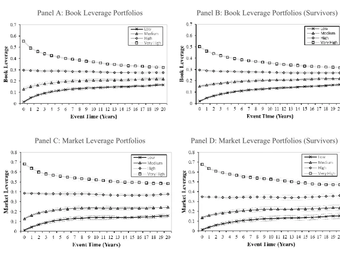
The methodology begins by studying the evolution of leverage for the cross-section of firms, through an “event-study” framework. Figure 1 presents the evolution of the average leverage ratios of quartiles in event time, using the following methodology. Each calendar year, firms are sorted into four portfolios according to their “raw” leverage ratios: Low, Medium, High and Very High. The year of the portfolio formation is considered the event year 0. Afterwards, it is computed the average leverage ratios for each portfolio in the subsequent 20 years. holding the portfolio composition constant (but for firms that exit the sample). For example, in 1990, four portfolios are formed by ranking firms based on their actual leverage ratios and it is calculated the portfolio’s yearly average leverage from 1990 to 2009, holding the portfolio composition fixed. This process of sorting and averaging is repeated for each calendar year, which results in 39 sets of event-times averages. The method is conducted for book and market leverage. The solid lines of the figure exhibit the average leverage of the actual leverage portfolios in event time, whereas the surrounding dashed lines represent 95% confidence intervals.3
3 The confidence interval is defined as a two-standard error around the mean. The standard error is performed as the average standard error for the total sets of averages in each portfolio event year. The lower bound is calculated by subtracting the mean for the confidence interval. The upper bound is the sum of the previous two parameters.
10
Figure 1: Average leverage of actual leverage portfolios in event time. The sample consists of all nonfinancial firm-years observations available in the Compustat database between 1980 and 2018. The figures are constructed in the following manner. Each calendar year, quartiles are formed by ranking firms based on their leverage ratios and it is computed the four portfolios average leverage ratios in the subsequent 20 years, holding their composition constant (but for firms that exit the sample). Event year 0 is the year of portfolio formation. Each panel presents the evolution of leverage ratios for each portfolio (Low, Medium, High and Very High) in event time. Panel A and C represent the evolution for book and market leverage portfolios for the primary sample, respectively. Panel B and D represent the book and market leverage portfolios evolution, by this order, for a subsample denominated Survivors, required to have at least 20 years of nonmissing data on book leverage. The surrounding dashed lines represent 95% confidence intervals. The variables construction is detailed in the Appendix.
Several characteristics are common across all graphs. First, there is a significant cross-sectional dispersion in the portfolio’s formation period, as illustrated by the considerable distance between quartiles at event year zero. Second, there is a markedly convergence between the four portfolios average leverage ratios over time. Third, most of this convergence seems to occur in the first 5 years of the portfolios. The former aspect is mainly evidenced by the steepening curve during the initial years in Very High, Medium and Low portfolios. Lastly, the differences among the four portfolios persist across the 20 years, which suggests the presence of a permanent or long-run component in leverage ratios.
Panel B: Book Leverage Portfolios (Survivors) Panel A: Book Leverage Portfolios
11
Figure 1, Panel A (Panel C) show the average evolution of book (market) leverage ratios for the four portfolios over the 20 years in the primary sample. At the year of the portfolio formation, the average book (market) leverage ratios in the Very High, High, Medium and Low portfolios are 55% (68%), 30% (39%), 13% (13%) and 2% (1%), respectively. Thus, on average, the differential across quartiles is 18% (22%). After 20 years, the book (market) leverage ratios in the Very High, High, Medium and Low portfolios are 32% (48%), 27% (38%), 22% (24%), 17% (16%), respectively. Hence, the mean dispersion between book (market) leverage portfolios at the final year is 5% (11%), and it declined 13% (11%) since the portfolio formation, revealing the existence of a mean reversion tendency in leverage ratios. The mean book (market) leverage throughout all years in the Very High, High, Medium and Low portfolios are 39% (53%), 28% (37%), 20% (22%), and 13% (12%), respectively.
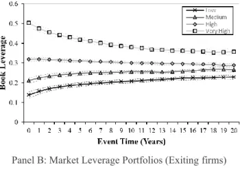
A potential concern when interpreting the main sample figures is the effect of survivorship bias. As years advance further away from the portfolio formation period, firm wills progressively drop out the sample as a result of bankruptcy, acquisitions or buyouts. Furthermore, given that the time period ends in 2018, it is only possible to analyse 20 years length portfolios until 1999. To address the latest limitation, the former analysis is repeated for the subsample Survivors. As Figure 1, Panel B (Panel D) shows, the average book (market) leverage ratios of the portfolios in event time for this sample display similar patterns. At event year zero, the mean differential, across book (market) leverage ratios quartiles, is 16% (22%). This average dispersion between book (market) leverage portfolios narrows to 5% (11%) at the last event year. Despite the convergence, the leverage differences across the portfolios 20 years later remain very persistent. Concerning the changes in the sample composition shortcoming, it is conducted an “event-study” for a subsample only including firms which leave the sample at any point to verify the effect of dropouts. Thus, the main sample is restricted to only include firms which have the last nonmissing value in leverage before 2018 – the last year of this study time horizon. Later, firms are again sorted into quartiles according to their actual leverage ratios on a yearly frequency, but it is computed the evolution of the average portfolio’s last value in leverage, conditional on the last observation occurring before 2018, in the following 20 years, instead of their leverage ratios. The value of leverage ratios on firms just prior exiting the sample is considered a reasonable proxy for future leverage ratios by Lemmon et. al (2008). Figure A1, in Appendix, shows that the patterns slightly change using this procedure, revealing that the leverage ratios of firms before exiting the sample are similar to the leverage ratios of the broader sample of firms. Indeed, both the permanent and the transitory component are yet observable. Hence, firm exit does not seem to drive the patterns of Figure 1.
12
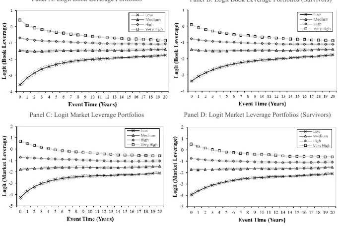
A second concern is that, because leverage only takes values within the closed unit interval, the mean leverage may tend to reflect away from the extremes zero and one (Chang and Dasgupta, 2009 and Elsas and Florysiak, 2015). To examine this possibility, the leverage is transformed using a logit function, such that:
𝐿𝑜𝑔𝑖𝑡(𝐿𝑒𝑣𝑒𝑟𝑎𝑔𝑒𝑖𝑡) = ln ( 𝐿𝑒𝑣𝑒𝑟𝑎𝑔𝑒𝑖𝑡 1 − 𝐿𝑒𝑣𝑒𝑟𝑎𝑔𝑒𝑖𝑡) .
However, a drawback of this method is that it cannot be applied to the values of the extremes. Therefore, leverage ratios exactly equal to 0 or 1 are ruled out of this analysis. This comprises 14.8 (28.0) percent of the observations for book (market) leverage in the main sample. Figure A2, in Appendix, plots the outcomes for book and market leverage resultant from this transformation of leverage for the primary sample and for the Survivors subsample. Even though the scale is different, the figures are nearly identical to those exhibited by Figure 1. Thus, the transitory component exhibited in Figure 1 does not appear to result from the fractional nature of leverage.
A final concern with the Figure 1 is the possibility of its process of sorting mostly captures the variation of underlying factors associated with leverage, rather than the “pure” leverage (e.g., High/Low portfolio corresponds to big/small companies). As the Table A1, in Appendix, demonstrates, leverage is highly correlated with some commonly used leverage determinants, namely firm size or tangibility. Following the approach of Lemmon et.al (2008), firms are sorted based on a different criterion. Each calendar year, a regression with leverage as dependent variable and a set of 1-year lagged traditional factors (Rajan and Zingales, 1995) as independent variables is run. These factors are firm size, profitability, market-to-book and tangibility.4 Also included on this regression are industry indicator variables (Fama and French
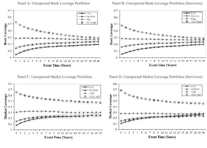
38-industry classifications). Based on the residuals produced by these regressions, firms are allocated into the four portfolios. The residuals of these regressions are denominated as “unexpected leverage”. This exercise is again repeated for each calendar year of the timespan, generating 39 sets of event-times averages. As previously, the same procedure is performed for the book and market leverage in both samples. The solid lines of the figure exhibit the average actual leverage of each portfolio in event time, while the dashed lines display the 95% confidence intervals.
4 It is also examined the effects of using a sorting procedure based on a different specification, inspired by Frank and Goyal (2009), which adds to the regressions the following variables: industry median leverage, dividend payer and cash flow volatility. Figure A3, in Appendix, shows that the results do not change considerably.
13
Figure 2: Average leverage of unexpected leverage portfolios in event time. The sample comprises all nonfinancial firm-years observations available in the Compustat database between 1980 and 2018. Each calendar year, firms are sorted into quartiles by ranking their “unexpected leverage” and then it is computed their average actual leverage ratios in the next 20 years, holding the portfolio fixed. Unexpected leverage corresponds to the residuals of a regression of leverage on a set of 1-year lagged independent variables. These independent variables are firm size, profitability, market-to-book and tangibility. Also included in the regression are industry indicator variables (Fama and French 38 industry classification). The solid lines in each panel present the evolution of leverage ratios for each portfolio (Low, Medium, High and Very High) in event time. The dashed lines represent 95% confidence intervals. Event year 0 is the year of portfolio formation. Panel A (Panel C) represents the book (market) leverage evolution for all firms. Panel B (Panel D) represents the book (market) leverage for the Survivors firms. The variables construction is detailed in the Appendix.
Two outcomes are expected from the Figure 2 process of sorting. The first is a short-run phenomenon, where it is expected less variation in the portfolio formation period. The second is a long-run phenomenon, in which any differences between portfolios should quickly disappear.
Figure 2, Panel A and C report the event-time evolution of “unexpected leverage” portfolios among the main sample. In the portfolio formation, the average differential across book (market) leverage portfolios is 16% (19%), while at event year 20, the previous measure is 3% (7%). Hence, in the portfolio formation the mean differential decreased 2 percent for
Panel A: Unexpected Book Leverage Portfolios Panel B: Unexpected Book Leverage Portfolios (Survivors)
14
book leverage and 3 percent for market leverage in comparison with Figure 1. In addition, the dispersion at the final year of portfolios narrowed 2 percent for book leverage and 4 percent for market leverage. Therefore, the abovementioned expectations are visible, but at a small scale for book leverage, which is consistent with the findings in Lemmon et.al (2008). This indicates that most of the variation of the book leverage is found in the residual of the specification. Counterintuitively, similar conclusions are extracted for market leverage. Although the anticipated phenomena are more visible in relation to book leverage, there are still leverage differences between the four portfolios in the formation period. Differences that persist throughout the 20 years, except for the Low and Medium portfolios. The Medium portfolio is only (very slightly) surpassed by the Low portfolio at event year 18 in the primary sample. In turn, Figure 2, Panel B and D, unveil similar findings regarding the subsample analysis. The difference is that portfolios converge more rapidly, due to the lower number of observations. Concerning the market leverage portfolios (Panel D), the Medium portfolio is outstripped by the Low at the midpoint. Thus, after removing the heterogeneity of traditional determinants of capital structure, despite the increased convergence, portfolios leverage differences remain highly persistent.
Three conclusions arise from this analysis. Firstly, traditional determinants seem to not account for as much variation as previously expected. Secondly, it indicates that a crucial factor containing a permanent and a transitory component is missing from existing models of leverage as suggested in Lemmon et.al (2008). Lastly, it shows that these authors findings persist for a recent period containing the subprime crisis.
4.2. The Persistent Component of Leverage
Figures 1 and 2 insights show that leverage ratios seem to be characterized by a permanent and a transitory component. This subsection is segmented in five analysis that further examine the permanent feature. First, it is measured the impact of initial leverage ratios in future leverage ratios. Secondly, two analysis are conducted to gauge the leverage variation. The first is the computation of the within- and between-firm variation of leverage and the second are variance decompositions, which allow to quantify the explanatory power of existing determinants as well as test for the presence of firm fixed effects. Thirdly, it is run a distributed lag model of leverage to find if the results hold using a model that allows short and long-term fluctuations through lengthier range lags. Afterwards, it is studied how far back this feature goes, focusing the analysis on an IPO subsample. This subsection concludes by examining the vulnerability of the results to the specification (Pooled OLS or Firm Fixed Effects model) used.
15 4.2.1. The Impact of Initial Leverage
The permanent feature present in former figures indicates that firms’ future leverage ratios are strongly related with their initial leverage ratios. However, this misses a quantitative evidence. To enhance the previous analyses, it is estimated the following regression that allows to quantify the importance of initial leverage ratios on future leverage:
𝐿𝑒𝑣𝑒𝑟𝑎𝑔𝑒𝑖𝑡 = 𝛼 + 𝛽𝑋𝑖𝑡−1+ 𝛾𝐿𝑒𝑣𝑒𝑟𝑎𝑔𝑒𝑖0+ 𝜈𝑡+ 𝜀𝑖𝑡,
where 𝑖 indexes firms; 𝑡 indexes years; 𝑋 is a set of 1-year lagged control variables; 𝐿𝑒𝑣𝑒𝑟𝑎𝑔𝑒𝑖0
is firm 𝑖´s initial leverage, which is proxied for the first nonmissing value for leverage; 𝜈 is a year fixed effect; and 𝜀 is a random error term. The first observation of each firm is removed of the analysis to avoid an identity at time zero. The key coefficient of the regression is 𝛾. It estimates the importance of initial leverage ratios in determining future leverage ratios. Considering the figures, 𝛾 represents the average leverage differences across firms throughout time. The inclusion of control variables permits to measure the relative importance of firm’s initial leverage ratios vis-à-vis determinants frequently considered by the literature.
Table 2 shows the output of this regression. Each coefficient is scaled by the corresponding variable’s standard deviation in order to ease their interpretation. In other words, the coefficients in the body of the table measure the change in leverage resulting from a one-standard deviation change of either Initial Leverage or a given control variable.
Table 2 reports the estimations of equation (1) for book and market leverage using the entire sample. Column [1] considers a model with neither control variables nor year fixed effects, merely including the variable Initial Leverage. In this specification, a one-standard deviation change in Initial Leverage is associated with an average change of 8% (6%) in future values of book (market) leverage. Both standardized coefficients are highly significant (t-statistics of 52.34 and 29.27, respectively), which is consistent with Figure 1. Column [2] presents a model using a set of determinants suggested by Rajan and Zingales (1995) as well as calendar year fixed effects. The estimates for 𝛾 demonstrate a small economic change of Initial Leverage from 8% to 6% in the case of book leverage and from 6% to 5% for market leverage. Regarding statistical significance, this independent variable continues very significant. Specifically, it remains the most important determinant for this model in book leverage. In turn, different results are extracted for market leverage. It is still a crucial determinant of future market leverage ratios, but it is outperformed by other determinants. The last column adds to the previous model variables considered in Frank and Goyal (2009). Most of the variables added (1)
16
present statistically significant marginal effects, yet they do not diminish as much as expected neither the statistical significance nor the economic magnitude of Initial Leverage. Indeed, the prior variable is the second most important determinant for book leverage and it persists considerably significant for market leverage, applying this specification.
Ultimately, the estimates demonstrate that historical leverage consists of a crucial determinant of future leverage even after controlling for other factors, mainly for book leverage. More importantly, the results are in line with the behaviours illustrated in previous Figures, although this consists of a more rigorous test of persistence in leverage, because it enables the determinants, except Initial Leverage, to update in each period.
Table 2
The Initial Leverage Effect on Actual Leverage
The sample consists of all nonfinancial firm-years observations available in the Compustat database between 1980 and 2018. The body of the table presents the following measures: the variables coefficients, scaled by the standard deviation, and the respective t-statistics for each parameter (in parentheses), the presence or absence of Year Fixed Effects, as well as the adjusted R-squares and the number of observations for each specification. The first columns present a model only considering Initial Leverage, the second columns present a specification including variables motivated by Rajan and Zingales (1995), whereas the third columns show estimates for a model containing the determinants considered in Frank and Goyal (2009). All variables are trimmed at the upper and lower 0.5-percentiles. T-statistics are robust to clustering at the firm level and heteroskedasticity. Variables construction details are in the Appendix.
All Firms
Book Leverage Market Leverage
Variable [1] [2] [3] [1] [2] [3] Initial Leverage 0.08 0.06 0.05 0.06 0.05 0.03 (52.34) (41.42) (33.21) (29.27) (28.27) (21.61) Log (Sales) 0.03 0.03 0.04 0.04 (20.98) (20.74) (20.51) (17.35) Market-to-book -0.02 -0.01 -0.09 -0.07 (-19.98) (-11.98) (-55.83) (-52.09) Profitability -0.02 -0.02 -0.04 -0.03 (-21.71) (-22.66) (-27.65) (-25.52) Tangibility 0.04 0.03 0.08 0.04 (31.40) (20.10) (37.52) (23.44)
Industry Median Lev 0.07 0.12
(47.60) (54.08)
Cash Flow vol. 0.00 0.00
(-0.40) (-2.26)
Dividend Payer -0.03 -0.04
(-21.38) (-23.62)
Year Fixed Effects No Yes Yes No Yes Yes
Adj. R2 0.14 0.21 0.29 0.04 0.27 0.38
17
Table A2, in Appendix, presents the outputs of the equation (1) for book and market leverage in the Survivors subsample. It shows that the results for Survivors are in line with the primary sample. Initial Leverage continues as the second-best predictor of future book leverage ratios, again only surpassed by Industry Median Book Leverage. Nonetheless, the analysis for this subsample strengthens the quality of the estimates, because it deals with the survivorship bias inherent to the main sample. It has a median lag time for Initial Leverage of 13, which is substantially higher than the 3.5 median lag time present in the core sample, given that Survivors firms have a median number of time-series observations of 26. Thereby, it concludes that leverage 13 years ago is a major determinant in actual levels of leverage.
4.2.2. The Leverage Variation
The second part of the study of the persistent component of leverage starts with a nonparametric variance decomposition. The within-firm and between-firm variation of leverage are determined, using the xtsum command in Stata. Book (market) leverage exhibits a within-firm variation of 14.2% (23.0%) and a between-within-firm variation of 20.1% (30.2%). Therefore, the between-firm variation is 42% and 31% larger than the within-firm, for book and market leverage respectively. These results are in line with the findings of Graham and Leary (2011), who stated that most variation is cross-sectional, rather than time-series. More importantly, they are consistent with the patterns displayed by the figures of the firm’s cross-sectional evolution of leverage study.
The following step of the analysis to gauge the variation of leverage is to perform an analysis of covariance (ANCOVA), which permits to decompose the variation in leverage attributable to each factor. Following the approach of Lemmon et.al (2008), justified by the large number of firms and computer memory limitations, it is formed a random subsample with 10% of the initial companies and performed its variance decomposition. To increase the accuracy of the estimates, the process of sampling and performing a variance decomposition is repeated 20 times by specification.5 The final coefficient is the average of all trials. The model
estimated is the following:
𝐿𝑒𝑣𝑒𝑟𝑎𝑔𝑒𝑖𝑡 = 𝛼 + 𝛽𝑋𝑖𝑡−1+ 𝜂𝑖 + 𝜈𝑡+ 𝜀𝑖𝑡,
5 This was the number of trials chosen due to time constraints and computer memory limitations. However, an even higher frequency is recommended to minimize sampling errors.
18
where 𝑋 is a set of 1-year lagged control variables, 𝜂 is a firm fixed effect and 𝜈 denotes calendar year fixed effects.
Table 3 presents the results of the variance decompositions using seven specifications of leverage. The coefficients embodied in the table correspond to the fraction of the total partial sum of squares for a given model, id est, the partial sum of squares of a single variable is divided by the aggregate partial sum of squares of all parameters. This forces the columns to sum to one, easing the measurement of the relative importance of each variable. The last row of the table reports the adjusted R-Squares corresponding to each model, a crucial parameter to establish the conclusions for this analysis.
Column (a) demonstrates that the firm-specific effects solely capture most of the variation of leverage, given the adjusted R-square of 60 (66) percent for book (market) leverage. Columns (b) reveal that less than 5% of total leverage variation is captured when we switch to a model only including time fixed effects. This fortifies the conclusion that most of variation in leverage results of invariant factors. Therefore, leverage models only accounting for time-varying factors provide little insights about the heterogeneity of capital structures. Columns (d) and (e) present specifications including variables considered by Rajan and Zingales (1995), without and with firm fixed effect respectively. The first includes Industry FE. In turn, columns (f) and (g) report the results for models inspired by Frank and Goyal (2009). Regarding the specifications of Rajan and Zingales (1995), if we do not include fixed firm effects, Industry FE and Tangibility (Market-to-book) explain most of the variation of book (market) leverage. However, this model explains only 17% (31%) of the total variation present in book (market) leverage. When the former model is augmented with fixed effects, the adjusted R-square more than triples for book leverage and it is 2.29 times higher for market leverage. The specifications motivated by Frank and Goyal (2009) reveal similar results. When firm fixed effects are disregarded, Industry Median Leverage is the determinant with higher explanatory power. Nonetheless, the adjusted R-square increases significantly from 26% to 65% for book leverage and from 38% to 72% for market leverage, after including firm fixed effects.
The findings of this parametric test are twofold. It corroborates that leverage contains an important unobserved firm-specific component not captured by leverage determinants and it shows that most of leverage variation is cross-sectional. Nevertheless, this does not imply that current identified determinants fail to explain variation in leverage, although they present a small explanatory power. It is correct that column (e) with a specification including traditional determinants and firm fixed effects only raises the adjusted R-square by 3 (5) percent for book (market) leverage in relation to the specifications only including Firm FE of column (a).
19
However, the model of column (f) shows that variables without firm fixed effects still explain a considerable portion of the variation in leverage. Thus, this may just indicate that most of the explanatory power of existing determinants comes from cross-sectional, as oppose to time-series variation. Effect that is removed when firm fixed effects are included in the model.
Table 3
Variance Decompositions
The sample includes all nonfinancial firm-years observations available in the Compustat database from 1980 to 2018. The table displays the coefficients for different model specifications. The numbers in the body of the table, excluding last row, are computed dividing the partial sum of squares of that variable by the total partial sum of squares of the model, forcing each column to sum to one. Firm FE are firm fixed effects. Year FE are calendar year fixed effects. Industry FE are industry indicator variables (Fama and French 38 industry classification). Variables construction is detailed in the Appendix.
Book Leverage Market Leverage
Variable (a) (b) (c) (d) (e) (f) (g) (a) (b) (c) (d) (e) (f) (g) Firm FE 1.00 . 0.99 . 0.96 . 0.94 1.00 . 0.99 . 0.95 0.93 Year FE . 1.00 0.01 0.11 0.01 0.03 0.01 . 1.00 0.01 0.11 0.02 0.07 0.02 Log (Sales) . . . 0.06 0.01 0.08 0.01 . . . 0.02 0.01 0.05 0.01 Market-to-book . . . 0.07 0.00 0.02 0.00 . . . 0.37 0.01 0.26 0.02 Profitability . . . 0.07 0.01 0.05 0.01 . . . 0.04 0.01 0.04 0.01 Tangibility . . . 0.31 0.01 0.12 0.01 . . . 0.11 0.00 0.07 0.00 Industry med lev . . . . . 0.49 0.02 . . . 0.33 0.01 Cash flow vol . . . 0.00 0.00 . . . 0.00 0.00 Dividend payer . . . 0.11 0.00 . . . 0.10 0.00 Industry FE . . . 0.39 . 0.10 . . . . 0.35 . 0.09 Adj.R2 0.60 0.01 0.61 0.17 0.63 0.26 0.65 0.66 0.03 0.67 0.31 0.71 0.38 0.72 4.2.3. Managers Reactions to Short-Run and Long-Run Fluctuations
Several empirical works studied the speed of adjustment of firms’ capital structure. Results are inconclusive. Whereas some papers estimated a fast speed of adjustment (e.g, Flannery and Rangan, 2006 and Antão and Bonfim, 2012), others state that it is slower (e.g, Huang and Ritter, 2009 and Yin and Ritter, 2018). The variance decomposition outcomes suggest that managers respond slowly to changes in 𝑋 on Leverage. If this is the case, equations that only regard a one-period lag length in control variables, as equation (2), may provide an incomplete explanation of firms’ capital structure choices. To test this hypothesis, it is undertaken an alternative specification where control variables have deeper lags, such that:
𝐿𝑒𝑣𝑒𝑟𝑎𝑔𝑒𝑖𝑡 = 𝛼 + ∑𝑛𝑠=1 𝛽𝑠𝑋𝑖𝑡−𝑠+ 𝛾𝐿𝑒𝑣𝑒𝑟𝑎𝑔𝑒𝑖0+ 𝜈𝑡+ 𝜀𝑖𝑡,
where 𝑛 corresponds to the lag order of an explanatory variable inserted in 𝑋. This dissertation aims to compare its results with the ones obtained in Lemmon et. al (2008). As such, it replicates (3)
20
a lag length of 8 periods. The first observation for each firm is dropped to avoid an identity at time zero.
Table 4 presents the results of equation (3) using two summary measures: the short-run and the long-run multiplier. The first is the product of the coefficient estimated for a one-lagged period of the variable and the variable’s corresponding standard deviation. The second is the sum of the previous process across all eight lags. The interpretation of a long-run multiplier of 0.03 (e.g) is that a one-standard deviation change in that variable causes a 3% change in the equilibrium level (i.e., long-run) of leverage.
Table 4 reports the output of the model using the main sample. It shows that the responses of leverage to short-run and long-run variation in its determinants differ. Some factors produce a higher short-run impact in leverage such as Log (Sales) in the case of book leverage and Log (Sales), Tangibility or Cash Flow Volatility, in what concerns market leverage. Conversely, some parameters may cause a greater long-run response in leverage, as the case of Market-to-Book, Profitability and Industry Median Leverage regarding book leverage, or even being indifferent to both impacts (e.g. Dividend Payer). Moreover, it indicates that a model considering a long-run impact still struggles to explain differences, given that the portion of leverage variation captured by the determinants lagged eight periods is substantially smaller than the leverage unconditional standard deviation, that is of 22% (35%) for book (market) leverage, as shown by Table 1. For instance, Industry Median Leverage, the main determinant of future leverage ratios, long-run multiplier for book leverage is less 27% (6%/22%) than the unconditional standard deviation of book leverage. This shows that commonly used determinants explain a relatively small fraction of the total variation of leverage regardless if one uses a short- or long-run model. Furthermore, Initial Leverage remains significant in a model that accounts for short- and long-term fluctuations. Consequently, Initial Leverage is an important predictor of future leverage ratios, even if managers can respond to short-run and long-run changes in determinants. Table A3, in Appendix, documents the estimates for Survivors and concludes qualitatively similar findings.
21 Table 4
Short-Run versus Long-Run
The sample comprises all nonfinancial firm-years observations in the Compustat database from 1980 to 2018. This table presents the results of a distributed lag model of leverage. All the independent variables, expect Initial Leverage, have a lag length of eight periods. For each one it is shown the short-run and the long-run multiplier. The short-run multiplier is the product of the coefficient of the independent variable and its corresponding standard deviation. The long-run multiplier is the sum of all the eight standardized coefficients. Year fixed effects signal the presence (or absence) of calendar year fixed effects. The t-statistics are computed using standard errors robust to clustering at the firm level. All variables are trimmed at the upper and lower 0.5-percentiles. The variable Log (Sales) is detrended by using the residuals from a regression of Log (Sales) on a time trend to ensure that it is stationary, as in Lemmon et. al (2008). The Appendix details the construction of all variables.
All Firms
Book Leverage Market Leverage
Variable Short-Run Long-Run Short-Run Long-Run
Initial Leverage 0.03 0.03 (15.07) (11.66) Log (Sales) 0.05 0.03 0.05 0.04 (8.47) (4.08) (6.43) (4.90) Market-to-book 0.00 -0.02 -0.05 -0.10 (-3.70) (-16.46) (-28.86) (-80.25) Profitability -0.02 -0.03 -0.02 -0.04 (-12.09) (-24.54) (-13.12) (-31.20) Tangibility 0.03 0.03 0.05 0.04 (9.15) (7.05) (10.61) (8.92)
Industry med lev 0.04 0.06 0.07 0.12
(23.55) (39.61) (24.89) (46.39)
Cash flow vol. -0.01 0.01 -0.04 0.00
(-0.78) (1.18) (-3.77) (-0.90)
Dividend payer -0.02 -0.02 -0.04 -0.04
(-14.75) (-12.72) (-19.07) (-16.83)
Year fixed effects Yes Yes
Adj.R2 0.29 0.44
22 4.2.4. How Far Does the Persistent Component Go?
Considering that the focus is now to study how far back the firm-specific effect can go, the unexpected leverage portfolios will be formed at the time of the IPO. As a result, the main sample is restricted to only include firms with an IPO date.
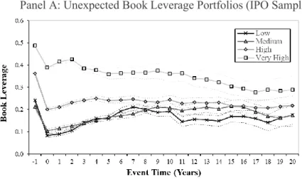
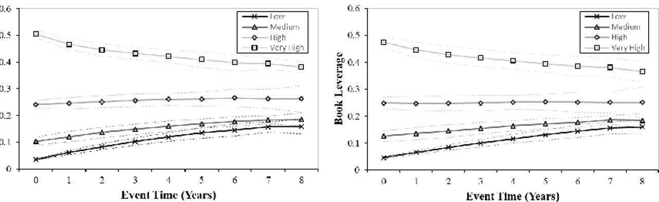
The methodology will follow the same reasoning behind Figure 2. Accordingly, it adopts a sorting procedure based on the “unexpected leverage”, but in a slightly different manner due to the lower number of observations (5,629 IPO firms). Firms are sorted into quartiles according to the residuals of a cross-sectional regression of initial leverage on initial values for firm size, profitability, market-to-book and tangibility. The initial values (leverage) correspond to the average variables’ values during the first three public observations in leverage. In other terms, each variable is computed as the average of its values over the event years 0 (IPO year), 1 and 2. This averaging process helps to mitigate the subsample outliers. In these regressions are still included calendar year fixed effects, that allow the distinction of the effects of IPOs in hot versus cold markets, as well as industry fixed effects at the event year 0. Figure 3 displays the actual leverage of the four portfolios in event time, where the event year 0 is the IPO year. Panels A and B exhibit the results for book leverage and market leverage, respectively. Concerning book leverage, the pre-IPO year (i.e., event year -1) is also incorporated to explore the speculation impact. Figure 3 reveals noteworthy features. This different setting continues showing a notably distance between portfolios and a mean reversion tendency, that does not impede the portfolio differences of persisting for a long period. The main change in relation to previous figures is that the Low and the Medium portfolios are now almost undistinguishable since the beginning, which may result of the reduced number of observations.
Moreover, the book leverage results reveal that the leverage differences were established prior to the IPO. The event year -1 presents a differential between the Very High and High portfolios of 12 percent and a distance from the High to the Medium portfolio of approximately 15 percent. Although these differences are striking, the leverage in the year before the IPO may not be representative of the firm’s leverage as private, but simply a consequence of the speculation effect. Despite this potential concern, this evidence suggests that higher (lower) levered private companies remain as such after going public. More importantly, it indicates that firms maintain their capital structure choices regardless of the widely known IPO bottlenecks such as changes in the firm’s control that may lead to agency problems, changes in the access to capital markets or the different information environment.
23
Figure 3: Average leverage of unexpected leverage portfolios in event time (IPO sample). The sample includes all nonfinancial firm-years observations available in the Compustat database between 1980 and 2018 which have an IPO year. Event year 0 is the IPO year. Firms are sorted into quartiles according to their “unexpected leverage” and then it is computed the actual leverage of the portfolios in event time. In this case, unexpected leverage is the residuals of a regression of initial leverage on initial values for the variables firm size, profitability, market-to-book and tangibility. Initial leverages/values are an average of the first three public years. The solid lines in each panel present the evolution of leverage ratios for each portfolio (Low, Medium, High and Very High) in event time. The dashed lines represent 95% confidence intervals. Panel A (Panel B) portray the results for book (market) leverage. Calendar year fixed effects and industry indicator variables (38 Fama and French industries) are included in the regressions. Both categorical variables are measured at the time of the IPO. The construction of the variables is detailed in the Appendix.
Panel A: Unexpected Book Leverage Portfolios (IPO Sample)