Abstract
An adaptation of the conventional Lanczos algorithm is proposed to solve the general symmetric eigenvalue problem K λKG in the case when the geometric stiffness matrix KG is not necessarily posi‐
tive‐definite. The only requirement for the new algorithm to work is that matrix K must be positive‐definite. Firstly, the algorithm is pre‐ sented for the standard situation where no shifting is assumed. Sec‐ ondly, the algorithm is extended to include shifting since this proce‐ dure may be important for enhanced precision or acceleration of convergence rates. Neither version of the algorithm requires matrix inversion, but more resources in terms of memory allocation are needed by the version with shifting.
Keywords
Lanczos algorithm, general eigenproblem, shear buckling.
Adaptation of the Lanczos Algorithm
for the Solution of Buckling Eigenvalue Problems
1 INTRODUCTION
One of the most efficient methods for extracting eigenpairs eigenvalues and eigenvectors was proposed by Lanczos Lanczos, 1950 . Lanczos algorithm is considered today to be the most efficient if not the most efficient numerical method for computing extreme eigenvalues and associated eigenvectors Paige, 1971; Paige, 1972 for large problems. The finite arithmetic of computers introduce some difficulties in the procedure since it may lead to loss of orthogonality of the eigenvectors being computed. However, the loss of orthogonality can be treated through corrective schemes Parlett and Scott, 1979 already available.
In structural modal analysis the eigenvalue problem to be solved is usually not in the standard form A λ, where A is a symmetric matrix. Because of inertial effects, in addition to the stiffness matrix K, there is always a mass matrix M involved, such that the eigenvalue problem is stated as K λM, known as the generalized form. In modal analyses the stiffness matrix is guaranteed to be positive semi‐definite, whereas the mass matrix is positive‐definite Ericsson and Ruhe, 1980; Ramaswamy, 1980; Bathe 1996 . Nevertheless, the traditional linearized buckling analy‐ sis requires computation of a geometric stiffness matrix KG, which is dependent on the prebuckling stress distribu‐
tion Zienkiewicz, 1991 . In the linearized buckling analysis matrix KG replaces matrix M. However, the positive‐
definiteness of KG is not guaranteed what brings apparently unsurmountable an obstacle to the conventional
Lanczos algorithm applied to the generalized eigenproblem. Jones and Patrick Jones and Patrick, 1989 propose the use of a spectral transformation to solve buckling eigenproblems, but it relies on a shifted operator and does not address the basic difficulty of taking the square root of a possibly negative number, except by taking preventive ac‐ tion of selecting appropriate initial guess vectors that must be preconditioned. However, if KG is indefinite, their
method crashes.
Given the incapacity of the conventional Lanczos algorithm to handle indefinite matrices KG this work proposes
an adaptation of the algorithm to compute eigenvalues critical loads in linearized buckling problems. The strategy consists basically in relying on the positive‐definiteness of K, despite the fact that KG is indefinite. Initially, a version
of the adapted algorithm is proposed without shifting that is sufficient to obtain the lowest positive eigenvalues usu‐ ally sought. Subsequently, a version of the algorithm with shifting is proposed in order to either enhance precision
Alfredo R. de Fariaa
a Instituto Tecnológico de Aeronáutica,
Department of Mechanical Engineering, São José dos Campos, SP, Brazil [email protected]
http://dx.doi.org/10.1590/1679‐ 78253932
or accelerate rates of convergence. It is shown that the version with shifting requires more computer resources in terms of memory allocation.
2 THE ADAPTED LANCZOS ALGORITHM
The generalized linear eigenvalue buckling problem is
1
where K is the stiffness matrix, is the eigenvector, λ is the eigenvalue and KG is the geometric stiffness matrix. K is symmetric and positive‐definite. KG is symmetric but may not be positive‐definite. In classical linearized buckling
analysis when there is only compressive prebuckling loads matrix KG can be assumed to be positive‐definite. How‐
ever, this is not always the case. Structural components subject to shear loads invariably lead to indefinite KG matri‐
ces. Two simple examples of these situation are panels subject to shear and closed box beams subject to torsion, both of which consist of practical cases encountered in aircraft wing design. Nonetheless, even compressive loads may result in indefinite KG matrices. Almeida and Hansen 2000 investigated rectangular composite plates with
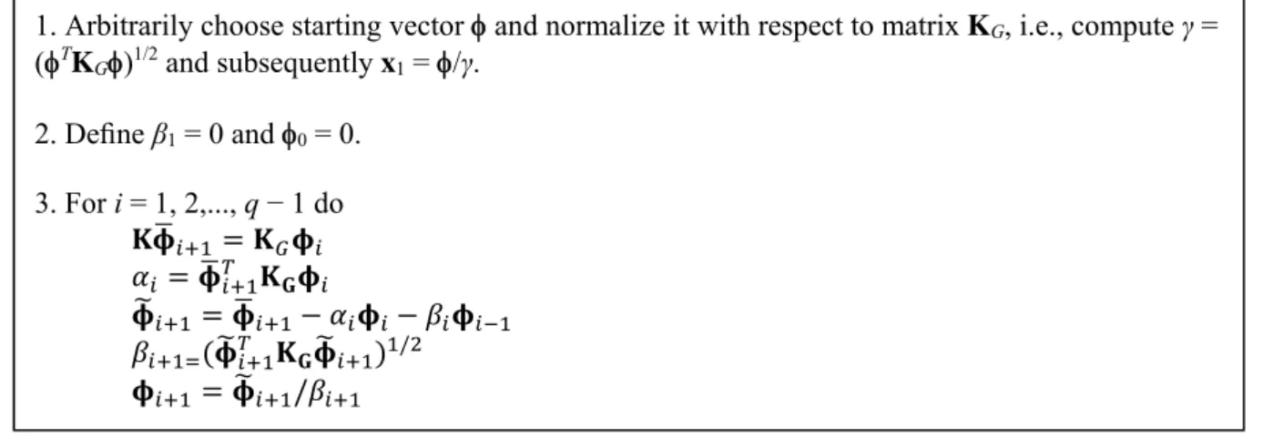
circular cutouts and observed local buckling modes related to negative eigenvalues. The absolute values of those negative eigenvalues were high in comparison to the positive eigenvalues. Even though these negative eigenvalues are not of practical relevance, they cripple the traditional Lanczos algorithm that will eventually be required to com‐ pute the square root of a negative number as will be shown. Figure 1 presents the traditional Lanczos algorithm proposed by Bathe Bathe, 1996 to solve the generalized eigenvalue posed in Eq. 1 .
Figure 1: Algorithm 1.
The algorithm in Fig. 1 generates a sequence of vectors i, at least theoretically, orthonormal to KG. As q in algo‐
rithm 1 increases, the symmetric tridiagonal matrix
⋱
2will possess eigenvalues that converge to the inverse of the eigenvalues of the original problem. In theory, it is shown that, when q is exactly the dimension of the eigenvalue problem, matrix T given in Eq. 2 will have eigenval‐ ues that are exactly the inverse of those of the original eigenproblem.
Observe that, in step 3 of algorithm 1, matrix products like TKG must be computed and, subsequently, their
square roots must be taken. In the case of buckling problems KG is indefinite, therefore, TKG may be negative, fatal‐
ly crippling the algorithm. If one insists in using the conventional algorithm and takes, instead, the square root of the absolute value of TKG , the algorithm flies off and converges to absolutely meaningless results. If the inverted ei‐
genvalue problem KG = υK is solved instead, where υ 1/λ, matrix products of the form TK would be computed and, because K is positive‐definite, it would lead necessarily to a positive number. Since the conventional Lanczos
1. Arbitrarily choose starting vector and normalize it with respect to matrix KG, i.e., compute γ =
(TK
G)1/2 and subsequently x1 = /γ.
2. Define β1 = 0 and 0 = 0.
3. For i = 1, 2,..., q− 1 do
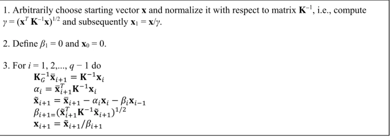
The fundamental aspect to be noted in proposing a new variant of the Lanczos algorithm is to realize that, since K is positive‐definite, its inverse, K 1, is also positive‐definite. One can therefore define the transformation
3 that is always unique because K is positive‐definite, therefore invertible. Substitution of Eq. 3 into Eq. 1 and pre‐ multiplication by KG 1 yields
4 There is apparently one inconsistency in Eq. 2 : KG is indefinite and may be singular, such that KG 1 may not
even exist. Let us forget this inconsistency for now and employ the conventional Lanczos algorithm to the eigenproblem posed in Eq. 4 .
Figure 2: Algorithm 2
The difficulty of having to take the square root of a negative number is now resolved since the product xTK 1x results in a positive number. However, the algorithm presented in Fig. 2 is apparently highly awkward because both K 1 and KG 1 are required. If one carefully examines the algorithm it will be clear that inversions are unnecessary. The inverse of KG is required only in the evaluation of that can also be recast as .
Therefore, KG 1 is not actually needed. As for K 1, notice that only products of the form K−1x are required. These
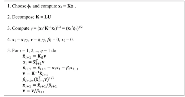
can be more effectively evaluated if recast as K x. Numerical solution of this system is achieved through tradi‐ tional LU decomposition of K Crout, Cholesky, etc. . Before beginning algorithm 2, matrix K can be LU decomposed and, since it is symmetric, only L must be stored. Refinement of algorithm 2 results in algorithm 3 presented in Fig. 3.
Vector v is only auxiliary. Computation of v in step 5 , is obtained through solution of the system , which is not troublesome since matrix K has already been LU decomposed. A particularly effective way of selecting the starting vector 1 is to make it equal to the main diagonal of matrix K. Since the transformation pro‐ posed in Eq. 3 was adopted, the eigenvectors of the original and transformed problems are related by i K 1xi.
The eigenproblem with shifting is posed in Eq. 5
5 where σ is the shift and the eigenvalues µ to be determined satisfy µ λ σ. If the transformation proposed in Eq.
3 is used in Eq. 5 , pre‐multiplication by KG 1 leads to
6 1. Arbitrarily choose starting vector x and normalize it with respect to matrix K1, i.e., compute
γ = (xT K1x)1/2 and subsequently x1 = x/γ.
2. Define β1 = 0 and x0 = 0.
3. For i = 1, 2,..., q− 1 do
Figure 3: Algorithm 3
The particularly complicated matrix product is purposely not computed. Both K 1 and KG 1 in this product are not actually evaluated in the algorithm proposed in Fig. 4. However, matrix, K σKG , is
now present and it must be LU decomposed. The adapted Lanczos algorithm with shifting is:
Figure 4: Algorithm 4
In algorithm 4 it is suggested that the two sequences of eigenvectors xi and i are stored. This procedure pre‐ cludes the necessity to solve systems of the form K x. However, if computer memory is scarce, then either x or only may be stored. Storing the sequence of i makes more sense since these are the eigenvectors of the original
eigenvalue problem. Computer memory may also become an issue because, in addition to K and KG, matrix K σKG
decomposed must also be stored. Another source of hardship may be the decomposition of K σKG. If the shift σ is
near one of the eigenvalues of the problem stated in Eq. 1 , K σKG may become singular, therefore not invertible.
3 NUMERICAL EXAMPLES
1. Choose 1 and compute x1 = K1.
2. Decompose K = LU
3. Compute γ = (x1TK1x1)1/2 = (x1T1)1/2
4. x1 = x1/γ, v = 1/γ,
1 = 0, x0 = 0.5. For i = 1, 2,..., q− 1 do
/ / /
1. Choose 1 and compute x1 = K1.
2. Decompose (K
KG) = LU3. Compute γ = (x1T1)1/2
4. x1 = x1/γ, 1 = 1/γ,
1 = 0, x0 = 0 = 0.5. For i = 1, 2,..., q− 1 do
1 0 0 0 3 0 0 0 5
0 0 0 0 0 0 0 0 0
0 0 0 4 00 2
and
1 0 0
0 1 0
0 0 1
0 0 0 0 0 0 0 0 0
0 0 0 1 00 1
7
Since KG is indefinite, this simple problem helps illustrating the obstacles encountered by the conventional
Lanczos algorithm presented in Fig. 1. The starting vector is chosen as
1/√5 1/√5 1/√5 1/√5 1/√5 8
Blunt application of algorithm 1, requires, in the first iteration, evaluation of β22 0.1181, halting the algo‐ rithm. Stubbornly taking the square root of the absolute value of / to compute βi 1 does not help; it does not fix the algorithm. In this simple example this procedure would lead to the wrong set of eigenvalues 1.3409, 0.3819, 0.8515, 0.0392 and 0.0809. On the other hand, algorithm 3 produces the correct eigenvalues and eigen‐ vectors placed columnwise:
0001 . 0 0008 . 0 0003 . 0 7071 . 0 0000 . 0 0000 . 0 5000 . 0 0000 . 0 0006 . 0 0003 . 0 0000 . 0 0000 . 0 4472 . 0 0002 . 0 0002 . 0 5774 . 0 0000 . 0 0000 . 0 0.0000 0.0003 0005 . 0 0006 . 0 0003 . 0 0000 . 0 1.0000 and 3.0000 4.0000 5.0000 2.0000 1.0000 9
If one makes the geometric stiffness matrix KG indefinite by, for instance assuming that
1 0 0
0 0 0
0 0 1
0 0 0 0 0 0 0 0 0
0 0 0 1 00 1
10
then the new variant of the Lanczos algorithm delivers the solution
0000
.
0
0000
.
0
7071
.
0
0000
.
0
0.0016
5000
.
0
0000
.
0
0000
.
0
0005
.
0
0.0004
0005
.
0
0000
.
0
0000
.
0
4472
.
0
0.0000
0000
.
0
5774
.
0
0000
.
0
0000
.
0
0.0000
0007
.
0
0000
.
0
0023
.
0
0.0000
1.0000
and
4.0000
10
4.7661
2.0000
5.0000
1.0000
16 11Notice the "infinite" eigenvalue obtained numerically 4.76611016 and the correct eigenvector associated to it column 4 .
A more practical example consists of a 40 cm 40 cm square composite plate whose laminate is just a single layer of T300‐5208 graphite/epoxy properties in Tab. 1 of 0.15 mm thickness. The single layer is oriented accord‐ ing to angle θ as shown in Fig. 5. Simply supported boundary conditions are imposed along the four edges and pure shear loading is applied.
Property Value
Longitudinal modulus of elasticity E1 154.0 GPa
Transverse modulus of elasticity E2 11.13 GPa
In‐plane Poisson ratio 12 0.304
In‐plane shear modulus G12 6.98 GPa
Transverse shear modulus G13 G12 6.98 GPa
Transverse shear modulus G23 3.36 GPa
Figure 5: Single ply composite square plate.
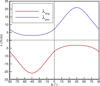
The composite plate is modeled with a 4 4 mesh of bicubic elements Faria, 2000 , and the stiffness and geo‐ metric stiffness matrices are computed. The Lanczos algorithm 3 for θ 45o leads to the critical loads 20.91 N/m
lowest positive eigenvalue and 3.17 N/m highest negative eigenvalue . Along the plate diagonal, where x y, the pure shear load induces compressive normal stresses. Therefore, a high critical buckling load is expected 20.91 N/m . When the layer angle is θ 45o the critical loads become 3.17 N/m lowest positive eigenvalue and 20.91 N/m highest negative eigenvalue .
Figure 6 shows how the lowest positive eigenvalue λpos and highest negative eigenvalue λneg vary with the layer angle θ. λpos and λneg have the same absolute values for θ 0o and θ 90o. The maximum |λ| is obtained for θ 45o. If the plate is required to equally support either positive or negative shear loads then the optimal strategy would be to choose θ 0o or θ 90o.
Figure 6: Critical load variation.
4 CONCLUSIONS
A deeper investigation of the Lanczos algorithm applied to the solution of the eigenvalue problem stated in Eq. 3 reveals that the principal contribution to vector xi+1 is from i, where i is the eigenvector related to the ith least ei‐ genvalue in absolute value. Hence, vector x2 consists mostly of 1; vector x3 consists mostly of 2; so on so forth, where the eigenvalues are ordered such that |λ1| < |λ2| < ... < |λn|. Thus, one expects that the procedure converges quickly to the least eigenvalues in absolute value and related eigenvectors. If a structure is subject to loadings in either direction positive or negative , the relevant critical buckling load is the one associated to the least eigenvalue in absolute value. Therefore, it is clear that eigensolvers of practical relevance must be able to compute eigenvalues of either sign.
References
(o)
(N
/m
)
-90 -75 -60 -45 -30 -15 0 15 30 45 60 75 90 -25
-20 -15 -10 -5 0 5 10 15 20 25
Bathe, K‐J., 1996 . Finite Element Procedures, Prentice Hall New Jersey .
Ericsson, T., Ruhe, A., 1980 . The spectral transformation Lanczos method for the numerical solution of large sparse generalized sym‐ metric eigenvalue problems. Mathematics of Computation 35: 1251‐1268.
Faria, A.R., 2000 . Buckling optimization of composite plates and cylindrical shells: uncertain loading combinations, Ph.D. Thesis, Uni‐ versity of Toronto.
Jones, M.T., Patrick, M.L., 1989 The use of Lanczo’s method to solve the large generalized symmetric definite N eigenvalue problem. NASA Contractor Report 181914, ICASE Report No. 89‐69.
Lanczos, C., 1950 . An iteration method for the solution of the eigenvalue problem of linear differential and integral operators. Journal of Research of the Natural Bureau of Standards 45: 255‐282.
Paige, C.C., 1971 . The computation of eigenvalues and eigenvectors of very large sparse matrices, Ph.D. Thesis, University of London. Paige, C.C., 1972 . Computational variants of the Lanczos method for the eigenproblem. Journal of the Institute of Mathematics and its Applications 10: 373‐381.
Parlett, B.N., Scott, D.S., 1979 . The Lanczos algorithm with selective orthogonalization. Mathematics of Computation 33: 217‐238. Ramaswamy, S., 1980 . On the effectiveness of the Lanczos method for the solution of large eigenvalue problems. Journal of Sound and Vibration 73:405‐418.