University of Uberlândiaas a fulfillment of the requirements for the PhD degree in the area of Artificial Intelligenceof the course ofGraduation in Electrical Engineering.
José Romildo Malaquias
Computer Algebra in Modern Functional
Languages
Prof. Dr. Antônio Eduardo Costa Pereira
Thesis SupervisorUniversidade Federal de Uberlândia
Uberlândia, MG
Brazil
Dados Internacionais de Catalogação na Publicação (CIP) M237c Malaquias, José Romildo, 1967-
Computer algebra in modern functional languages / José Romildo Malaquias. - 2007.
140 f. : il.
Orientador: Antonio Eduardo Costa Pereira.
Tese (doutorado) – Universidade Federal de Uberlândia, Programa de Pós-Graduação em Engenharia Elétrica.
Inclui bibliografia.
1. Inteligência artificial - Teses. 2. Programação funcional (Computa-ção) - Teses. I. Pereira, Antonio Eduardo Costa. II. Universidade Federal de Uberlândia. Programa de Pós-Graduação em Engenharia Elétrica. III. Título.
CDU: 681.3:007.52
Languages
José Romildo Malaquias
Composition of the Examining Board
Prof. Dr. Antônio Eduardo Costa Pereira FEELT – UFU Supervisor
Prof. Dr. Luciano Vieira Lima FEELT – UFU
Prof. Dr. Carlos Roberto Lopes FACOM – UFU
Prof. Dr. José Lopes de Siqueira Neto DCC – UFMG
Prof. Dr. Claudio Cesar de Sá DCC – UDESC
Sumário x
Abstract xi
Acknownledgments xii
1 Introduction 1
1.1 Computer Algebra . . . 1
1.2 Motivation . . . 3
1.3 Objectives . . . 4
1.4 Features of the Haskell Language . . . 6
1.5 History . . . 7
1.6 Text Structure. . . 10
2 Algebraic Formulas 12 2.1 Kinds of Formulas . . . 12
2.2 Trivial Representation of Formulas . . . 14
2.3 Extensible Union Types . . . 19
2.4 An Extensible Type Representation for Formulas . . . 21
2.5 Formula Representation with Existentially Quantified Type Variables . . . . 23
2.6 Abstract Data Types . . . 30
2.7 Basic Functions over Formulas. . . 31
2.7.1 Integer Formulas . . . 31
2.7.2 Constant Formulas . . . 32
2.7.3 Variable Formulas . . . 33
2.7.4 Indeterminate Formulas . . . 34
2.7.5 Application Formulas . . . 35
2.8 Canonical Form . . . 39
2.9 Representing Success and Failure . . . 41
3 Context 43 3.1 Formula Manipulation . . . 43
3.2 Controlling the Evaluation of Formulas . . . 45
3.2.1 The Need of Controllers. . . 45
3.2.2 Representing Contexts . . . 46
3.2.3 The Meaning of Some Controllers . . . 46
3.2.4 Referential Transparency . . . 53
3.2.5 Passing the Context as Input to Algorithms . . . 54
3.3 Implicit Parameters . . . 56
3.4 Alternative Solutions for Passing a Context Around . . . 57
4 Addition 59 4.1 Basic Addition Rules . . . 59
4.2 Addition of Integer and Rational Numbers . . . 60
4.3 Handling of Special Cases . . . 61
4.4 The Core of Addition . . . 64
5 Multiplication and Subtraction 74 5.1 Basic Multiplication Rules . . . 74
5.2 Multiplication of Integers . . . 75
5.3 Handling of Special Cases . . . 76
5.5 Additive Inverse and Subtraction . . . 85
6 Exponentiation and Division 88 6.1 Mathematical Background . . . 88
6.2 Basic Algorihtms for Powers . . . 89
6.3 Special properties of exponentiation . . . 93
6.4 Division . . . 99
7 System Organization 104 7.1 Module Organization . . . 104
7.2 Extending the Library . . . 107
7.3 Comparison to Other Systems . . . 109
8 Conclusions 113 8.1 Conclusions. . . 113
8.2 Future Work . . . 115
1.1 An opaque C program. . . 4
2.1 A first attempt in building a type representation for formulas. . . 14
2.2 Selectors. . . 16
2.3 Building a value of a data type. . . 16
2.4 Addition of two formulas . . . 17
2.5 Examples of addition of formulas. . . 17
2.6 Adding logarithms to the formula representation. . . 17
2.7 Addition od formulas, including derivatives. . . 18
2.8 Disjoint union of two types.. . . 19
2.9 Example of an extesible union type . . . 20
2.10 Subtyping relationship . . . 20
2.11 Subtyping relationship . . . 21
2.12 Representing the groups of application formulas . . . 21
2.13 Addition of formulas . . . 22
2.14 Extending the library of logarithms . . . 23
2.15 Existential type variables in data type declarations . . . 24
2.16 Context with existential type variables . . . 24
2.17 The general type of a formula using existential an type variable . . . 25
2.18 Integer formulas . . . 26
2.19 Constant formulas . . . 27
2.20 Sums . . . 28
2.21 Addition of formulas . . . 29
2.22 Integer functions. . . 32
2.23 Functions for handling constant values. . . 33
2.24 Selectors, constructors and predicates for variables. . . 34
2.25 Selectors, constructors and predicates for variables. . . 35
2.26 Functions for handling applications. . . 36
2.27 Constructors and selectors for basic applications. . . 38
3.1 Solutions of the quadratic equation. . . 45
3.2 One may represent contexts as records.. . . 47
3.3 State changing. . . 47
3.4 Procedural languages are not transparent. . . 54
3.5 Context as argument. . . 56
3.6 Implicit context. . . 57
3.7 Passing contexts around. . . 58
4.1 Addition of two terms. . . 62
4.2 An overloaded function for special addition rules. . . 63
4.3 Addition of logarithms. . . 64
4.4 The multiplication operator for formulas. . . 65
4.5 Theaddfunction. . . 66
4.6 Thefoldrfunction.. . . 66
4.7 ThemergeSumfunction. . . 69
4.8 ThemergeTermfunction. . . 71
5.1 ThemulFactorsfunction. . . 76
5.2 An overloaded function for special multiplication rules. . . 77
5.3 Multiplication of logarithms. . . 77
5.4 The multiplication operator for formulas. . . 78
5.5 Themulfunction. . . 79
5.7 ThemergeFactorfunction. . . 86
5.8 Thenegatefunction. . . 86
5.9 The subtraction operation. . . 87
6.1 Overloaded functions for special exponentiation rules.. . . 92
6.2 Power of two terms. . . 94
6.3 Power of two terms (continued). . . 94
6.4 Power of two terms (continued). . . 95
6.5 Power of two terms (continued). . . 95
6.6 Power of two terms (continued). . . 96
6.7 Power of two terms (continued). . . 96
6.8 Product of power. . . 97
6.9 Product of power: division . . . 97
6.10 Product of power: division by an integer . . . 98
6.11 Product of power: division by a sum . . . 100
6.12 Product of power: overloaded functions . . . 100
6.13 Prower of a product.. . . 101
6.14 Power of a power. . . 101
6.15 Radical. . . 102
6.16 Radical (continuation). . . 103
6.17 The division operation. . . 103
7.1 TDeriv in MatLab. . . 110
7.2 TDeriv in Mapple.. . . 110
7.3 TDeriv in Haskell (part one). . . 111
Muitos sistemas de computação algébrica foram propostos e implementados. A maioria deles
são implementados ou até mesmo implementam linguagens sem a propriedade da referência
transparencial, o que torna difícil e até mesmo impraticável a prova de correção de programas.
Esta tese apresenta um sistema de computação algébrica implementado como uma biblioteca
na linguagem de programação Haskell, que é uma linguagem funcional moderna com a
pro-priedade da referência transparencial desejada.
O autor apresenta os fundamentos e algoritmos básicos para manipulação de expressões
algébricas em um contexto declarativo, compatível com a Matemática.
Examina-se a adequação de construções oferecidas pela linguagem Haskell para a
imple-mentação da biblioteca de uma forma modular, de forma que ela possa ser facilmente estendida
com a inclusão de novas fórmulas algébricas e novas operações sobre fórmulas. Tais extensões
devem ser compatíveis com versões anteriores da biblioteca.
Esta tese também contribui por mostrar que linguagens funcionais modernas como Haskell
são viáveis para a programação de sistemas práticos, até mesmo podendo ser melhores que
linguagens convencionais em alguns aspectos, como nível de abstração.
Palavras Chave
Inteligência Artificial, Computação Algébrica, Linguagens Funcionais, Programação Funcional,
Many computer algebra systems have already been proposed and implemented. Most of them
are implemented in or even implement languages without the referential transparency property,
making it difficult, if not impractical, to reason about algebra programs. This thesis presents
a computer algebra system implemented as a library in the Haskell programming language, a
modern functional language with the desired referential transparency property.
The author presents the foundations and basic algorithms for manipulation of algebraic
ex-pressions in a declarative context, compatible with Mathematics.
The adequacy of the constructs provided by the Haskell programming language is
consid-ered when implementing such a library in a modular way, so that it can be easily extended
with the inclusion of new algebraic formulas and manipulations. Such extensions should keep
compatibility with prior versions of the library.
This work also contributes for showing that modern functional languages like Haskell are
viable for day to day programming, even beating conventional languages in some aspects, like
level of abstraction.
Keyworkds
Artificial Intelligence, Computer Algebra, Functional Languages, Functional Programming,
I am grateful to all the persons who, in different ways, have supported me in this project.
• First I am grateful to God for keeping me alive and for providing all the necessary
condi-tions for the development of this work.
• I am grateful to my wife Neli, for the encouragement when needed, and for the love all
the time.
• I am grateful to my children, Ana Carolina, Felipe e Luíza, who have understood why I
have stayed so many hours in front of a computer screen, instead of being with them for
more time.
• I am grateful to my parents, Dírcia Rosa and José Augusto, for bringing me to life and
for teaching me how to be a good person.
• I am grateful to Prof. Antônio Eduardo Costa Pereira, who helped me in the most difficult
momments when developing this work.
• I am grateful to all my friends and co-workers from the Computer Science Department at
the Federal University of Ouro Preto, for the friendship and for the years I was allowed
to be out doing this work.
Chapter
1
Introduction
1.1
Computer Algebra
Computers have been used for numerical computations since its beginnings. However these
general purpose machines can be used for transforming and combining symbolic expressions
as well. That is, computers can be used not only to deal with numbers, but also with abstract
symbols representing mathematical formulas. This fact has been realized much later and is only
now gaining acceptance among mathematicians and engineers.
Winkler [1] draws a good short introduction to Computer Algebra. Before 1850
mathe-maticians solved the majority of their problems by extensive calculations. However in the 19th
century the style of mathematical research changed from quantitative to qualitative aspects. The
advent of modern digital computers in general and by the development of program systems in
Computer Algebra, in particular. played a role on this shift. Although even in our days many
mathematicians think that the role of computers is number crunching and their role is the
appli-cation of the appropriate algebraic transformations to the problem, underestimating the power
of computing systems for algebraic manipulation, already in 1844 Lady Augusta Ada Byron,
countess of Lovelace, recognized that this division of labor is not inherent in mathematical
problem solving. In describing the possible applications of theAnalytical Enginedeveloped by Charles Babbage she wrote [1]:
"Many persons who are not conversant with mathematical studies imagine that
cause the business of [Babbage’s Analytical Engine] is to give its results in
nu-merical notation, the nature of its process must consequently be arithmetical and
numerical rather than algebraic and analytical. This is an error. The engine can
arrange and combine its numerical quantities exactly as if they were letters or any
other general symbols; and in fact it might bring out its results in algebraic notation
were provisions made accordingly."
And indeed computer is a "universal" machine capable of carrying out an arbitrary algorithm,
being it numerical, symbolic or of any other nature.
But what does one mean by Computer Algebra or symbolic algebra computation? R. Loos
wrote[2]:
"Computer Algebra is that part of computer science which designs, analyzes,
im-plements, and applies algebraic algorithms."
Algebraic algorithms are algorithms that transforms algebraic formulas (built from numbers,
variables and function applications) following the rules from Algebra, a field in the
Mathemat-ics.
So Computer Algebra systems deal not only with integers and reals, but also with
vari-ables representing unknown quantities and any expression combining numbers and varivari-ables by
means of mathematical operations. Numbers are represented exactly. The approximations of
floating point numbers for reals are not acceptable anymore. So there is no need to concern
about aproximation errors.
Computer Algebra software find its applications in any field dealing with the formulation of
lawsin mathematical terms, using algebraic equations and/or analytic concepts such as ordinary and partial differential equations and integral theorems. After the formulation of a law it should
1.2
Motivation
Nowadays there are many programs which perform Computer Algebra. These said programs
find applications in areas like Mathematics, Computer Sciences, Engineering, Economics, etc.
With these programs one can perform algebraic simplifications and handle literals, as shown in
the following examples.
5×a
2
−2ab+b2
a−b =5a+5b d
dx(ax
2+bx+c) =2ax+b
sin2a+cos2a=1
Most of these programs suffer from the drawback that their programming languages are not
referentially transparent, that is, they do not allow substitution of equals for equals, invalidating
the use of certain Mathematical laws. Even if other areas of thought are able to do without
substitution of equals for equals, this is not true of Mathematics, the main subject of Computer
Algebra. Therefore, the absence of referential transparency is a mortal sin, when it occurs in a
Computer Algebra language.
The notion of transparency is due to Whitehead and Russel [3]. Antoni Diller [4] illustrates
the invalidation of substitution in natural languages with the following sentence drawn from
Russell [5]:
George IV wished to know whether Scott was the author of Waverley.
In chapter3the reader will find a full account of this discovery of Russell’s. For the time
being, it should be noticed that the above sentence is true, since the mad king really wished
to know whether Scott was the author of Waverley. However, we do know that Scott and the
author of Waverley are indeed the same person. Therefore, we may feel entitled to substitute
Scott forthe author of Waverleyin Russell’s sentence. In doing so, we get
George IV wished to know whether Scott was Scott.
Imperative computer languages suffer from the same lack of transparency as a natural
lan-guage. For example, one cannot make use of the commutative property of multiplication
to conclude that the C program of listing 1.1 will print the same number twice, although
f(2)×g(5) =g(5)×f(2)in Mathematics. This happens in C because C functions may change the state of the computing system (by means of assignments to variables) besides (maybe)
com-puting a value. In program1.1 functiongchanges the contents of the global variablekbefore
returning a value and functionfneeds the value ofkin order to compute a result value. So calls
tog has an effect on calls tof. The return value of fdepends on the previous calls to g. This
program outputs-6=99.
Listing 1.1: An opaque C program.
#include <stdio.h>
int k = 1;
int g(int x)
{ k = k + x;
return k;
}
int f(int x)
{ return k - x;
}
void main()
{ printf("%d=%d\n", f(x)*g(x), g(x)*f(x)); }
So it is highly desirable that the language used to express the Computer Algebra algorithms
be referentially transparent.
1.3
Objectives
As has been noted, current Computer Algebra systems are implemented and/or support
imper-ative programming languages, which are based on state changing and consequently lack
refer-ential transparency. The author proposes to develop a new Computer Algebra system withouth
effects.
The purposes of this work are:
• to provide the basics for implementing a Computer Algebra system embeded in a modern
functional language, by implementing a small library of data types and functions for the
manipulation of algebraic formulas;
• to examine the adequacy of the Haskell language for the construction of a modular and
easily extendable library;
• to provide fundamental algorithms for manipulation of algebraic expressions in a
declar-ative context, compatible with Mathematics, that uses transparent languages.
Currently there is plenty of Computer Algebra systems, as the reader can find in section1.5.
Many of them are comercial products that resulted from many years of work of many skilled
developers. Those systems are very broad and complex, and find applications in many areas
and are too broad and complex, being already stablished tools for professional development.
It is not the intent of this work to provide a system that competes with them nor to provide a
complete package, since this would require many hours of several dedicated programmers. In a
first step, we hope to provide instead the implementation of a small library that can be used for the development of such system in the Haskell programming language.
A Computer Algebra system, due to its characteristics, is constructed in the following steps:
1. A group of people stablishes a core system capable of reading expressions of the domain
and comparing them for equality. The comparison should be semantic and not syntatic,
that is, expressions like 2∗yandy+yare considered equal. The same group of people also stablishes a programming language. The core system built in this way is proposed to
the comunity, together with simple examples like elementary integrations and derivatives,
etc.
2. If the proposed system is accepted, specialists from many areas of knowledge that require
symbolic manipulation start to add packages to the core system: more complex integrals,
is so broad that it is not feasible for the group who started the system to develop all the
packages. Also they would not have all the knowledge and ability to take this task.
A final user of a Computer Algebra system reading this text should keep in mind that it
describes only a starting core system, which is implemented by making use of some inovative
techniques related to the implementation language. Therefore users of Macsyma or
Mathe-matica (to mention a few successfull products) should not expect a description in this text of
a Computer Algebra system of the same level of those products, which are really products for
the final user. What is described here is only a core system embeded in a modern programming
language, which is not ready for the users, but should be further developed by the comunity if
accepted by the comunity. Then after some years of development it could become a system as
complete as Macsyma or Mathematica systems.
This project consist not only the design of a library in a given language, but also a study of
language constructs offered or even missing in the programming language in face of the needs
of the library. To accomplish this task some advanced knowledge of type systems and language
constructs that goes beyound undergraduate level are needed.
In asecond step, the library will be reimplemented in theCleanprogramming language[6], another modern functional language with a very good compiler, which will bring more
effi-ciency to the system. More specific algorithms, like derivatives, integrals, differential equations,
vectors and trigonometry, will also be implemented, making it suitable for application on real
world problems.
1.4
Features of the Haskell Language
The Haskell programming language have the following features:
• It is a modern functional language.
• It is strongly typed.
• Its type system is polymorphic, with
– parametric polymorphism and
– overloading polymorphism.
• A program is made up of a set of algebraic data type definitions and functions.
• There are high order functions.
• Functions can be defined by pattern matching.
• Lazy evaluation of expressions.
1.5
History
According to Nilsson [7], research in Computer Algebra had its beginnings when James Slagle
created the program SAINT, that was able to integrate functions by elementary methods. After
this first step, Joel Moses improved the algorithms of SAINT, creating another program of
symbolic integration which was named SIN.
In the sixties, Carl Engleman, Joel Moses and William Martin (at the Massachusetts Institute
of Technology, as part of the MAC project) started the projectMacsyma1[8], which is one of the finest systems of Symbolic Mathematics. It is quite large, and written in Lisp. After Macsyma,
many other systems of Computer Algebra came to light. Each of these systems tried to correct
a real or imaginary weakness of Maclisp, the original computer language of Macsyma. A few
of these systems are:
• Reduce2. In the beginning, Lisp had many dialects. In general, every machine had its own dialect. Macsyma was developed in Maclisp. Therefore, one could not build the
system in a machine running Franz Lisp, Interlisp, etc. The designers of Reduce [9][10]
proposed a standard dialect of Lisp, which should be portable to any machine. Although
Reduce became very popular, Standard Lisp was badly beaten by Common Lisp in the
1http://www.macsyma.com/
struggle to become the standard dialect of the main AI language. In the mean time,
Macsyma migrated from MACLISP to Common Lisp. The result is that Macsyma runs in
a standard language, while Reduce is built on top of an obscure dialect known as Standard
Lisp.
• Maple3. Lisp always had a bad reputation for being slow. Therefore, Maple [11] was developed (at the University of Waterloo, Canada) in a procedural language (C) with a
view to greater efficiency. Since procedural languages like C are not fit for symbolic
computation, the implementors of Maple were forced to invent a symbolic language. Not
being experts in compiler construction, they wrote an interpreter for the Maple language.
The result is that Maple is much slower than Macsyma and other Lisp based systems.
Maple’s source code is not in the public domain.
• Derive4. This package (and its precursorMuMATH) was designed to offer a small and fast Computer Algebra system [12]. It was the only competitor to Macsyma that really
delivered its promises. The system is indeed very small and reasonably fast. However, it
did not meet the commercial success of Reduce and Maple.
Maple, Reduce and Derive were designed to be worthy competitors of Macsyma. There are
also systems designed to offer limited functionality in a friendly environment. Among these
systems,MatLab5[13] andMathematica6[14] became imensily popular.
It is interesting to note that these two systems that promised limited functionality failed to
deliver their promise too. Due to demands from the market, the developers of both MatLab
and Mathematica increased the functionality of their systems, which became as fat as Reduce.
However, neither MatLab nor Mathematica have the well designed architecture of Reduce. In
fact, these system suffered from a chaotic growth.
Other systems are:
• Magma7. Magma is a large software package designed to solve computationally hard
3http://www.maplesoft.com/ 4http://www.derive.com/ 5http://www.mathworks.com/ 6http://www.mathematica.com/
problems in algebra, number theory, geometry and combinatorics. It provides a
mathe-matically rigorous environment for computing with algebraic, number-theoretic,
combi-natoric and geometric objects. Magma’s language is imperative with standard
imperative-style statements and procedures, but offers a functional subset providing closures,
higher-order functions, and partial evaluation.
• Axiom8. Axiom was originally developed as a research tool by IBM in collaboration
with experts around the world. The unique strength of AXIOM is derived from its
object-oriented approach and its overall structure which is strongly typed and hierarchical.
AX-IOM’s algebra library is built on Common LISP.
• Yacas9. Yacas, standing for Yet Another Computer Algebra System, is a small and
highly flexible Computer Algebra system and language. It is written in C++ and can be
embedded into other applications. Things implemented include arbitrary precision
inte-ger arithmetic, rationals, complex numbers, vectors, matrices, derivatives, Taylor series,
equation solving. It is being developed by Ayal Pinkus towards a symbolic calculator and
there are plans to have a user interface through an internet browser.
• Ginac10. Ginac is a C++ library for doing computer algebra. It allows symbolic ma-nipulation from within a C++ program. It is currently in active development, and looks
very promising. GiNaC is an iterated and recursive acronym for GiNaC is Not a CAS,
where CAS stands for Computer Algebra System. It is designed to allow the creation
of integrated systems that embed symbolic manipulations together with more established
areas of computer science (like computation- intense numeric applications, graphical
in-terfaces, etc.) under one roof.
• HartMath11. HartMath is a Computer Algebra system written in Java. All math
func-tionality is written in Java itself. HartMath has roughly the same funcfunc-tionality as Yacas.
Some of the main implemented features are big rational number arithmetic, symbolic
8http://www.iec.co.uk/symbolic_software.asp 9http://www.xs4all.nl/~apinkus/yacas.html 10http://www.ginac.de/
derivatives, linear algebra, plot functions, numeric functions, pattern matching rules and
pure functions.
• Jacal12. JACAL is an interactive symbolic mathematics program. JACAL can manipu-late and simplify equations, scalars, vectors, and matrices of single and multiple valued
algebraic expressions containing numbers, variables, radicals, and algebraic differential,
and holonomic functions. It is written in Scheme, a dialect of Lisp.
• Maxima13. Maxima is a Macsyma clone, licensed under the GPL (GNU General Public License). It can be found in the GNU repositories, and is written in Common Lisp. It
seems there is currently no maintainer for Maxima.
• MockMMA14. MockMMA is a Mathematica-style parser and pattern matcher, written in
Lisp, with some additional mathematical functionality. One can manipulate polynomials
in several variables over the integers, rational functions, and a variety of other
mathemati-cal objects. Manipulations include simplification, differentiation, integration, evaluation,
pattern matching, etc. It is implemented in Common Lisp.
1.6
Text Structure
This text is organized in six chapters.
Chatper one: Introduction Presents the motivation of this work and its objectives as well as
a brief history on the subject.
Chapter two: Formulas Explains how the data is organized in abstract types that describe
algebraic expressions or formulas.
Chapter three: Context Justifies the need of keeping a set of flags, called the context, which
are checked while doing the simplification of an algebraic formula, and provides
infor-mation to decide what kind of transforinfor-mations should be applied.
Chapter three: Addition Explains the fundamental algorithms of the system for addition.
Chapter four: Multiplication and Subtraction. Discusses the algorithms used in symbolic
multiplication and the use of the multiplication by -1 to achieve the subtraction.
Chapter five: Exponentiation and Division Presents the algorithms used both in
exponentia-tion and in division.
Chapter six: System Organization Presents the module structure of the system and the
re-sults of a benchmarking program.
Chapter seven: Conclusion and Future Work Presents the conclusion and suggestions for
Chapter
2
Algebraic Formulas
In this chapter, the reader will find descriptions abstract representations of the algebraic
expres-sions in our Computer Algebra library. The author will be specially concerned with the basic
manipulations of the foresaid expressions, but he will also discuss the result of computations
that may fail or succeed.
For the sake of clarity, the termformula will be used foralgebraic expression, as expres-sion is already used when discussing programming languages and denotes a construct of the language not necessarily related to Algebra. This avoids ambiguity in terminology.
2.1
Kinds of Formulas
Formulas are expressions that can be manipulated in Algebra. They can be added and
multi-plied. They can be squared. Trignometric transformations may be applied to them. They can be
diferentiated and integrated. A large number of operations can be applied to formulas. Formulas
may be composed by numbers and variables, which can be combined in different ways.
Formulas can be grouped, according to their structure, in several groups, including:
• Integers, corresponding to the integer numbers, as defined in axiomatic theories like
Peano’s axioms, Church’s numbers, or in one of the many brands of the Set Theory. A
few examples of this group are 416, 7453 and−3291.
• Constants, representing known mathematical entities. They are expressed by a symbol or
a name, likeπ,e(neperian number) andı(imaginary unit). In general, a constant formula stands for a number without an exact representation in a given numeric system.
• Variables, corresponding closely to mathematical variables. Logicians call them literals
more often than not. Examples of literals: x,y,a,b,α,β.
• Applications, which are formulas built from simpler formulas by applying a functional
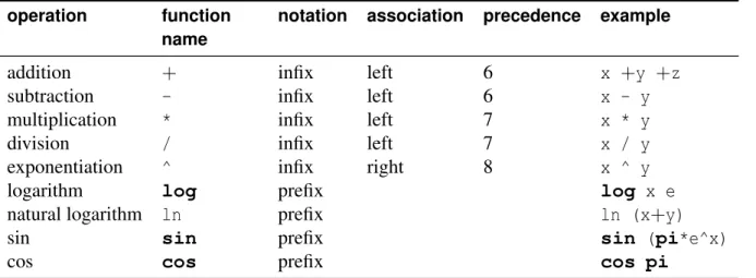
operator to its arguments, which are themselves formulas. Exemplos: sinx, cothx, lnx, log10x, x+2, −a, π2 and 5×sin[3π(α+2)]. Applications may have different forms, depending on the operator. The basic arithmetic applications are
– Sum, denoting the sum of two formulas. Examples area+band 13+y×4x.
– Product, denoting the product of two formulas. For example 4×x and(a+b)×
(a+c).
– Power, denoting the power of two formulas, as inx2and(a+b)12.
There is no need for special forms for differences and quotients: they can be expressed
using the above formulas. Basicaly, for any formulasxandy,
x−y = x+ (−1)×y x
y = x×y
−1
Other common applications are
– Logarithm of a formula in a given base. Examples are log10y, loge(x+y) and logbbc.
– Trigonometric formulas, like sine, cosine and tangent of a formula. Examples:
sinx, cosa2, tan(x2+y2).
There are many other possible forms of applications (hyperbolic formulas, derivatives,
• Indeterminates, which are formulas whose value cannot be determined, like those
ob-tained by dividing by zero. Examples are 3/0, 00and log0x.
2.2
Trivial Representation of Formulas
The representation of formulas in the implementation language is tricky. One could simply use
an algebraic data type to obtain the disjoint union of the relevant groups of formulas. Listing
2.1 is a first attempt in defining the type of formulas using this approach. It includes only the
Listing 2.1: A first attempt in building a type representation for formulas.
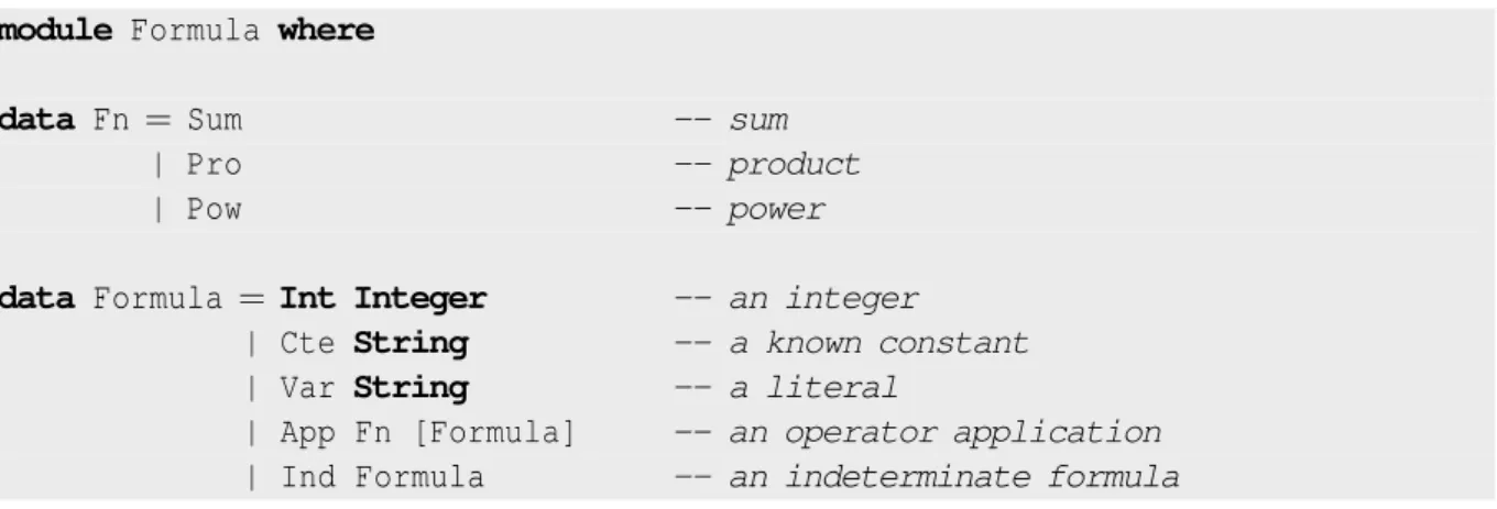
module Formula where
data Fn = Sum -- sum
| Pro -- product
| Pow -- power
data Formula =Int Integer -- an integer
| Cte String -- a known constant
| Var String -- a literal
| App Fn [Formula] -- an operator application
| Ind Formula -- an indeterminate formula
most basic groups of formulas: integers, named constants, variables, sums, products, powers
and indeterminates.
The declaration of an algebraic data type defines a possibly recursive type and the set of its
value constructors, specifying the types of the arguments of each constructor. For instance, type
Formulahas the following value constructors: Int,Cte,Var,App andInd. For example, the
contructorCte has a sole argument, of type String. ConstructorApp has two arguments of
typesFnandFormula.
Application formulas have a commom representation: an operator followed by a list of
arguments. The type of the operator,Fn, is simply an enumeration of all possible operators: in
this case sum, product and power. Each argument is a formula.
Table 2.1 exemplifies mathematical formulas and their corresponding representation by a
Math Haskell
831 Int 831
π Cte "pi"
x Var "x"
4+x Sum App [Int 4, Var "x"] a×x App Pro [Var "a", Var "x"]
x2×a App Pow [Var "x", App Pro [Int 2, Var "a"]]
x−y×z App Sum [Var "x", App Pro [Int (-1), Var "y", Var "z"]]
π/2 App Pro [Cte "pi", App Pow [Int 2, Int (-1)]] m/0 Ind (App Pro [Var "m", App Pow [Int 0, Int (-1)]])
Table 2.1: Representing mathematical formulas.
constructors) take a prefix form. This prefix form is somewhat harder to read, but it eases the
handling of expressions.
Note that the mapping between the integer representation and the integer field is constrained
only by the amount of memory available in the computer, as Hasekll’sIntegertype represents
arbitrary precision integers: its values can be as large as there is room for storing them in
memory. There is no fixed number of bits for representing them as it happens in conventional
languages like C, Pascal and Java.
One may deploy a constructor and its arguments as a pattern on the left hand side of
equa-tions used to define funcequa-tions in Haskell, as in any other language that uses Landin’s notation.
Listing2.2shows an example of using a constructor in a pattern. The patterns of listing2.2play
the role of selectors: they select components of a value of typeFormula. In this example the
selected component is one of the contructor arguments. Of course, this constructors can also be
used to build a value of the corresponding type. This is shown in listing2.3.
Listing 2.2: Selectors.
module Main where
import Formula
getName :: Formula→String getName (Int i) =show i getName (Cte name) = name getName (Var v) = v
getName (Ind x) = getName x getName (App fn args) = fnToString fn
where
fnToString Sum ="+"
fnToString Pro ="*" fnToString Pow ="^"
main :: IO ()
main =print (getName (Cte "pi"))
Listing 2.3: Building a value of a data type.
module Main where
import Formula
mkSum :: Formula→Formula→Formula mkSum x y = App Sum [x,y]
main :: IO ()
main =print (mkSum (Cte "pi") (Int 23))
Mathematics:
m+n = the sum ofmandn m,n∈Z
x+0 = x
0+x = x
(x+y) +z = x+y+z
x+ (y+z) = x+y+z
Listing2.5shows examples of application of the functionaddto some formulas.
Listing 2.4: Addition of two formulas add :: Formula→Formula→Formula
add (Int m) (Int n) = Int (m + n) add x (Int 0) = x
add (Int 0) x = x
add (App Sum xs) (App Sum ys) = App Sum (xs++ys) add x (App Sum ys) = App Sum (x:ys) add (App Sum xs) y = App Sum (y:xs) add x y = App Sum [x,y]
Listing 2.5: Examples of addition of formulas x1, x2, x3, x4, x5, x6 :: Formula
x1 = add (Int 81) (Int 12) -- Int 93
x2 = add (Cte "pi") (Int 0) -- Cte "pi"
x3 = add (Int 0) (Var "alfa") -- Var "alfa"
x4 = add (App Sum [Int 5, Var "x"])
(App Sum [Cte "e", Var "y"]) -- App Sum [Int 5, Var "x", Cte "e", Var "y"]
x5 = add (Var "x")
(App Sum [Int 7, Var "y"]) -- App Sum [Var "x", Int 7, Var "y"]
x6 = add (App Sum [Int 5, Var "x"])
(Cte "pi") -- App Sum [Int 5, Var "x", Cte "pi"]
easy extension of the type Formula without affecting all programs alreading using this type.
Certainly the library will not offer all possible groups of formulas and someone probably would
like to extended it. For example, suppose the library does not deal with logarithms and the user
wishes to add support for them (effectively extending the library). A new value constructor for
logarithms should be added in the definition of type Fn. Also new rules may need to be added
in the relevant function definitions. Listing 2.6 shows an updated definition for the type of
operators. Listing2.7 shows an extended addition operation capable of adding two logarithms
Listing 2.6: Adding logarithms to the formula representation.
data Fn = Sum -- sum
| Pro -- product
| Pow -- power
| Log -- logarithms
in the same base, according to the following mathematical law.
Listing 2.7: Addition od formulas, including derivatives.
add :: Formula→Formula→Formula
add (Int m) (Int n) =Int (m + n) add x (Int 0) = x
add (Int 0) x = x
add (App Log x b1) (App Log y b2) =if b1 == b2
then App Log [mul x y, y1]
else App Sum [App Log [x,b1], App Log [y,b2]] add (App Sum xs) (App Sum ys) = App Sum (xs++ys)
add x (App Sum ys) = App Sum (x:ys) add (App Sum xs) y = App Sum (y:xs) add x y = App Sum [x,y]
mul :: Formula→Formula→Formula mul = . . .
Many kinds of formulas and the related operations may be implemented in the library:
sums, products, powers, logarithms, trigonometric formulas (sine, cosine, tangent, etc.),
in-verse trigonometric formulas (arc sine, arc cosine, etc.), hyperbolic formulas, vectors, matrices,
equations, derivatives and integrals, among others. Extending the type of formulas with a new
constuctor for each new kind of formula will force the extension of the functions that manipulate
formulas. The source code of the library would have to be changed in many points to
accom-plish that, and the level of modularization would be less then acceptable. So an alternative
representation for formulas which make the library more modular is desirable.
Haskell 98, the current definition of Haskell, does not easily support data type extension
with new constructors and corresponding extensions of functions defined on this type with new
rules. Nonetheless most of Haskell implementations extends the language with new features
that are useful in solving this problem: instance overlapping and multiparameter type classes.
These and other common extensions to Haskell will be extensively used in the library. There is
2.3
Extensible Union Types
Subtyping is a relation between two types which stablishes that every value of the subtype is
also a value of the supertype. With the help of type classes we can introduce some kind of
subtyping in Haskell, as is suggested by Liang, Hudak and Jones in [15].
We begin with a discussion of a key idea in our framework: how formulas may be expressed
as extensible union types.
The disjoint union of two types is captured by the data type constructorEitherof listing
2.8. It is a polimorphic data type constructor pre-defined in Haskell.
Listing 2.8: Disjoint union of two types.
data Either a b =Left a
| Right b
Basicaly the typeEither a bis the disjoint union of typesaandb, where values of typea
are labeled withLeftand values of typebare labeled withRight. For exampleLeft True
andRight ’A’are instances of the typeEither Bool Char.
The unionEither a bcan be viewed as a supertype, and the summands typesaandbas
the subtypes.The operations that characterize the subtype relationship are
• injection of a value of a subtype into the supertype, which is accomplished by applying
one of the value constructorsLeftorRightto the original value, and
• projection of a value of the supertype into a subtype, which is done by pattern matching
the value of the supertype with one of the patternsLeft xorRight x; if the matching succeeds, then the projection also succeeds binding x to the projected value; otherwise the projection fails.
The projection may fail, as the target subtype may not be the correct type for the original value.
An extensible union may be arbitrarily nested to accomodate a set of the subtypes. For
example, the union of the types Integer, Char, [(Char,String)] and Int →Bool,
Listing 2.9: Example of an extesible union type
type T =Either Integer
(Either Char
(Either [(Char,String)]
(Int→Bool)))
The injections and projections discussed above only work if the exact structure of the union
is known. In order to have a single pair of injection and projection functions to work on all such
constructions, a type class is used to capture the summand/union type relationship, refered here
as a subtype relationship. The subtyping relationship between two types sub andsup will be
expressed making bothsub andsup an instance of the classSubType, defined in listing 2.10,
which introduces the functionsinj andprj. The success or failure of the projection function
Listing 2.10: Subtyping relationship
class SubType sub sup where
inj :: sub→sub -- injection
prj :: sup→Maybe sub -- projection
is represented by a value of typeMaybe sub:
• Just xfor a successful projection resulting inx, and
• Nothingfor a projection that fails.
The partial functionfromJustof typeMaybe a →adefined in the standard Haskell library,
can be used to access a successful result. Section 2.9 further discusses the representation of
success and failure.
Note that listing 2.10 is not valid Haskell 98 code, as SubType is a multiparameter type
class. However most Haskell implementations extend the language to include this feature.
Every typeais a subtype of the typeEither a b, as listing2.11shows. Also, every type
awhich is a subtype of typeb, is also a subtype of the typeEither c b.
The instance declarations appearing in listing2.11overlaps and are not allowed in Haskell
98. Again most Haskell implmentations extend the language to allow overlapping instances.
Now that we have the means to stablish the subtyping relationship between two types, we
Listing 2.11: Subtyping relationship
instance SubType a (Either a b) where
inj =Left prj (Left x) =Just x prj _ =Nothing
instance SubType a b => SubType a (Either c b) where
inj =Right . inj
prj (Right x) = prj x prj _ =Nothing
2.4
An Extensible Type Representation for Formulas
The representation introduced earlier for formulas will be kept, but the representation of
opera-tors of application formulas will be made an extensible union type, in order to easily accomodate
new kinds of application formulas. Listing 2.12 redefines theFn data type from listing2.1 as
an extensible union type. Each operator has its own type, distinct from the types of all other
Listing 2.12: Representing the groups of application formulas
newtype Sum = Sum
newtype Pro = Pro
newtype Pow = Pow
type Fn =Either Sum (Either Pro Pow)
instance SubType Pow Pow where
inj = id prj =Just
operators. The typeFnis a supertype of all operator types.
Listing2.13reimplements addition of formulas using this new types. Note how the rules
for specific kinds of applications being added are implemented: there is an overloaded function
calledaddAppwhich should be defined for each possible kind of application. It has three
argu-ments: the operator of the first formula, its arguments, and the second formula. This function
may succeed returning the sum of the formulas, or it may fail. The instance for Sum knows how
to sum two formulas where the first of them is a sum.
To extend the library with logarithms:
Listing 2.13: Addition of formulas add :: Formula→Formula→Formula
add (Int m) (Int n) = Int (m + n) add (Int 0) x = x
add x (Int 0) = x add (App op xs) y
| isJust u =fromJust u
where
u = addApp op xs y add x (App op ys)
| isJust u =fromJust u
where
u = addApp op ys x
add x y = App Sum [x,y]
class AddApp a where
addApp :: a →[Formula]→Formula→Maybe Formula addApp _ _ _ =Nothing
instance (AddApp a, AddApp b) => AddApp (Either a b) where
addApp (Left x) = addApp x addApp (Right x) = addApp x
instance AddApp Sum where
addApp Sum xs y@(App op ys)
| prj op ==Just Sum =Just (App (inj Sum) (xs++ys)) addOp Sum xs y =Just (App (inj Sum) (xs++[y])
instance AddApp Pro
2. Extend the type of operators, redefining theFntype.
3. Define versions of any overloaded functions for operators.
Listing2.14extends our small library with logarithms following the above steps.
Listing 2.14: Extending the library of logarithms
newtype Log = Log
type Formula =Either Log (Either Sum (Either Pro Pow))
instance AddApp Log where
addApp Log [x1,b1] y@(App op [x2,b2]) | prj op ==Just Log &&
b1 == b2 = Just (App (inj Log) [mul x1 x2,b1]) addApp _ _ _ =Nothing
In the next section the author introduces auxiliary functions for manipulating formulas,
turning them into abstract data types.
2.5
Formula Representation with Existentially Quantified Type
Variables
An alternative for representing extensible data types and functions relies on existentially
quan-tified type variables [16] and type classes. These combination leads to a style of programming
with similarities with the object oriented paradigm. Existential type variables are not part of
Haskell 98, although most Haskell implementations have it as an extension to the language.
An existential type variable is mentioned only in the value constructors and is not part of
the type constructor, allowing the construction of values of the same declared type, based on
arguments of unrelated types. Listing 2.15 shows an example of a data type declaration with
existential type variables. The components of the values cannot be accessed outside of the scope
of the type variable. This means that to have access to the components, functions have to be
attached to the value.
Listing 2.15: Existential type variables in data type declarations data Item = forall a . MkItem a (a→Bool)
f :: Item→Bool f (MkItem a f) = f a
x, y :: Item x = MkItem 5 even y = MkItem ’B’ isUpper z = MkItem False not
results :: [Bool]
results = [ f x, f y, f z ]
the functions defined by classes in the context can be used to handle the values. Listing 2.16
illustrates this technique.
Listing 2.16: Context with existential type variables data Item = forall a . (Eq a) => MkItem a (a→Bool)
f :: Item→ Item→Bool f (MkItem a f) (MkItem b g)
| a == b =False
| otherwise= f a || f b
x, y :: Item x = MkItem 4 odd
y = MkItem ’a’ isLower
result :: Boolean result = f x y
In order to represent the formulas, each kind of formula has its own data type declaration
and does not have to concern about how the other kinds of formulas are represented. Functions
handling each kind of expression should be also defined, again without concerning with every
other kind of formulas. These functions should be overloaded in order to keep the same interface
for handling any kind of formulas. In our example of addition of basic formulas, this means
that there should be a data type for integers, constants, variables, sums, another for products
and another for powers, toghether with one function for adding integers, another for adding
over the types of each kind of formula. The general type of a single formula can then be
expressed with an existential type variable and a context restricting the variable to instances of
classCFormula, as appears in listing2.17.
Listing 2.17: The general type of a formula using existential an type variable
class ( Eq f
, Show f , CInt f , CCte f , CSum f , CAdd f
, . . . {- classes for other formulas and operations -}
) => CFormula f where where
isEqual :: f→Formula→Bool isEqual _ _ =False
data Formula = forall f . (CFormula f) => Formula f
instance Show Formula where
showsPrec p (Formula f) =showsPrec p f
instance Eq Formula where
(Formula x) == y = isEqual x y
instance CFormula Formula where
isEqual (Formula f) = isEqual f
Each specific type of a formula should be an instance of classCFormula. In order to interact
with formulas of different kinds (like adding an integer to another integer, or to a constant, or to
a sum, and so on), each kind of formula may have corresponding type classes with overloaded
functions specific for the operations related to the kind of formula.
Listings2.18, 2.19 and 2.20 shows how some integers, constants and sums can be
repre-sented. Listing2.21has code for the addition operation.
To extend the library with a new kind formula or a new operation is done by
1. defining a new data type for the formula or a new function for the operation
2. defining a new type class for the formula or operation, with all relevant instance
defini-tions; defaults may be used for the kinds of formulas without a specific behaviour related
Listing 2.18: Integer formulas
newtype FInt = FInt Integer
deriving (Eq,Show)
mkInt :: Integer→Formula mkInt = Formula . FInt
class CInt f where
isInt :: f→Bool intVal :: f →Integer
--isInt _ =False
intVal =error "bug: intVal"
instance CInt FInt where
isInt _ =True intVal (FInt x) = x
instance CInt Formula where
isInt (Formula x) = isInt x intVal (Formula x) = intVal x
instance (CFormula a) => CInt a
instance CFormula FInt where
isEqual (FInt m) x = isInt x && intVal x == m
-- Some useful formulas
zero = mkInt 0 one = mkInt 1 two = mkInt 2 three = mkInt 3 four = mkInt 4 mOne = mkInt (-1)
Listing 2.19: Constant formulas
newtype FCte = FCte String
deriving (Eq,Show)
mkCte :: String→Formula mkCte = Formula . FCte
class CCte f where
isCte :: f→Bool cteName :: f→String
--isCte _ =False
cteName =error "bug: cteName"
instance CCte FCte where
isCte _ =True cteName (FCte x) = x
instance CCte Formula where
isCte (Formula x) = isCte x cteName (Formula x) = cteName x
instance (CFormula a) => CCte a
instance CFormula FCte where
isEqual (FCte n) x = isCte x && cteName x == n
-- Some useful formulas
pi = mkCte ":pi"
e = mkCte ":e"
i = mkCte ":i"
isPi x = isCte x && cteName x == ":pi"
isE x = isCte x && cteName x == ":e"
Listing 2.20: Sums
newtype FSum = FSum [Formula]
deriving (Eq,Show)
mkSum :: [Formula]→Formula mkSum = Formula . FSum
class CSum f where
isSum :: f→Bool terms :: f→[Formula]
--isSum _ =False
terms =error "bug: terms"
instance CSum FSum where
isSum _ =True
terms (FSum xs) = xs
instance CSum Formula where
isSum (Formula x) = isSum x terms (Formula x) = terms x
instance (CFormula a) => CSum a
instance CFormula FSum where
Listing 2.21: Addition of formulas add :: Formula→Formula→Formula
add x y
| isJust u =fromJust u
| isJust v =fromJust v
| otherwise= mkSum [x,y]
where
u = addT x y v = addT y x
class CAdd a where
addT :: a→ Formula→Maybe Formula addT _ _ =Nothing
instance CAdd FInt where
addT (FInt 0) x = Just x
addT (FInt m) x | isInt x = Just (mkInt (m + intVal x)) addT _ _ =Nothing
instance CAdd FSum where
addT (FSum xs) y | isSum y =Just (mkSum (xs++terms y))
| otherwise=Just (mkSum (xs++[y]))
instance CAdd Formula where
addT (Formula x) = addT x
3. adding the new type classes to the context of the CFormulatype class, making the new
functions available to all formulas through the generalFormuladata type.
Prior examples already ilustrates this process.
This solution is also based on other Haskell extensions: multiparametric type classes,
over-lapping instance declarations and undecidable instance declaractions. Some Haskell
implemen-tations provide all of them.
In a modular design, each kind of formula or specific operation should be definied in its
own module, making almost all of the modules of the library mutually recursive. The major
difficult found with this are related to deficiencies in the module system implementation. No
Haskell implementation correctly provides support for mutually recursive module definitions,
although it is a feature of Haskell. This was the reason why this solution to data type and
function extendibility was not adopted.
2.6
Abstract Data Types
Section 2.6 describes an algebraic data type that one can use to represent formulas. During
the development of a project, the programmer often has to add constructors, or to modify the
representation of a given type. When this happens, one must modify every single module which
happens to use the representation. For instance, if somebody renamesVartoV, an application
which makes use of the old name must undergo the appropriate changes. Besides this, in a
collective project, all participants would have to understand well the definition of every single
component of the whole. This may decrease productivity, since programmers must worry not
only about their own chores, but also with their collaborators decisions.
With abstract data types, one avoids the shortcomings of algebraic types by hiding the type
representation and other implementation details. A set of constructor functions, selectors and
predicates replace the constructor patterns of algebraic types. Haskell programmers should
resort to the module system in order to implement abstract data types. Only identifiers listed
in the export list of a module are visible outside of a module. Any other identifiers defined
order to hide the data type representation, the constructors should not be exported in the module
interface. This has the disadvantage of not being possible to define functions on the abstract data
type in client modules by pattern matching. In the absence of contructors to serve as patterns,
one cannot access the components of a structure through pattern matching. In fact, one cannot
even recognize the structure. The solution for this drawback is to export functions, which play
the role of constructors, predicates, and selectors.
The theory of abstract data types is quite old, from a time when pattern match and equational
definitions didn’t exist. Therefore, this otherwise powerful tool does not provide the handy
resources of pattern match, and forces the programmer to adopt a style that is at once old
fashioned and difficult to read. Nevertheless, the necessity of preserving contributions even
after modifying type declarations forces us to adopt abstract data types, and to make sure that
users of the library do not manipulate formulas directly, but only through exported functions.
Such functions are predicates for checking the kind of a formula, constructors for building a
new formula from its constituent parts, and selectors for accessing components of a formula.
The type abstract hides the implementation details from the users and keeps future changes in
the representation from propagating to contributed code.
2.7
Basic Functions over Formulas
2.7.1
Integer Formulas
In Section2.1, we have seen that integer formulas correspond to the mathematical integers. The
basic operations on integer formulas are:
mkInt :: Int →Formula
constructs an integer formula from an integer value;
intVal :: Formula →Int
selects the integer value from the integer formula, and
checks whether a formula is an integer formula.
In listing 2.22, the reader will find the Haskell definition of these three functions. Some
Listing 2.22: Integer functions. mkInt :: Integer→Formula
mkInt =Int
isInt :: Formula→Bool isInt (Int _) =True isInt _ =False
intVal :: Formula →Integer intVal (Int x) = x
zero, one, two, three, four, mOne :: Formula zero = mkInt 0
one = mkInt 1 two = mkInt 2 three = mkInt 3 four = mkInt 4 mOne = mkInt (-1)
isZero, isOne, isMOne :: Formula→Bool isZero (Int 0) =True
isZero _ =False
isOne (Int 1) =True isOne _ =False
isMOne (Int (-1)) =True isMOne _ =False
useful integers like zero and one are defined at this point, together with predicates for them.
2.7.2
Constant Formulas
Constant formulas correspond to special entities found in Mathematics for which there is no
direct and exact representation in the commonly used number systems. Examples of constants
are π, e (neperian number) and ı (imaginary unit). Listing 2.23 shows the definitions of the functions used to handle constants. These functions are:
mkCte :: String →Formula
cteName :: Formula →String
selects the name of the constant formula, and
isCte :: Formula →Bool
checks whether a formula is a constant formula
Listing 2.23: Functions for handling constant values. mkCte :: String→Formula
mkCte = Cte
isCte :: Formula→Bool isCte (Cte _) =True isCte _ =False
cteName :: Formula→String cteName (Cte x) = x
pi, e, i, mI :: Formula
isPi, isE, isI, isMI :: Formula→Bool
pi = mkCte ":pi"
isPi (Cte ":pi") =True isPi _ =False
e = mkCte ":e"
isE (Cte ":e") =True isE _ =False
i = mkCte ":i"
isI (Cte ":i") =True isI _ =False
mI = mkPro [mOne, i]
isMI x = isPro x && appArgs x == [mOne, i]
Some common constants are also defined, together with predicates for them.
2.7.3
Variable Formulas
Among other kinds of formulas, section2.1introduces the concept of a formula variable. It was
said in the previous section that variable values correspond to mathematical variables.
There-fore, they are primarily used to represent fixed, but unknown quantities. The basic constructors,
mkVar :: String →Formula
constructs a variable formula from a name that identifies the variable;
varName :: Formula →String
selects the name of the variable formula, and
isVar :: Formula →Bool
checks whether a formula is a variable formula.
In listing2.24, the reader will find the definitions that must be added to the implementation
module of the algebraic data types in order to handle formula variables.
Listing 2.24: Selectors, constructors and predicates for variables.
mkVar :: String→Formula mkVar = Var
isVar :: Formula→Bool isVar (Var _) =True isVar _ =False
varName :: Formula→String varName (Var x) = x
2.7.4
Indeterminate Formulas
Another kind of formula introduced in section2.1 is the indeterminate formula. Such formula
arises as the result of undefined operations, like division by zero, and do not represent any
mathematical object. Corresponding constructor, selector, and predicate functions are defined
for indeterminate formulas:
mkInd :: Formula →Formula
constructs an indeterminate formula from the original formula;
indFor :: Formula →Formula
isInd :: Formula →Bool
checks whether a formula is an indeterminate one
Listing2.25, defines these functions.
Listing 2.25: Selectors, constructors and predicates for variables. mkInd :: Formula→Formula
mkInd = Ind
isInd :: Formula→Bool isInd (Ind _) =True isInd _ =False
indFor :: Formula →Formula indFor (Ind x) = x
2.7.5
Application Formulas
Representation
Integer, variable and constant formulas are atomic and cannot be decomposed into constituent
parts. Application formulas are made of simpler formulas, combined by means of functions.
They represent mathematical operations that have not been carried out (simplified), possibly
because there is no way to simplify them or the user does not want it in a simplified form. Some
basic application formulas are sums, products and powers, which are essentials to any treatment
of applied Algebra.
Their representation is discussed in section 2.4. Basically, an application formula has an
operator and a list of arguments. The type of the operator is an extensible union type. See
listing2.12.
The constructor, the two selectors, and the predicate associated to application formulas are
given below. Their definitions are given in Listing2.26.
mkApp :: Fn →[Formula] →Formula
constructs an application formula from an operator and a list of formulas (the arguments
appFn :: Formula →Fn
selects the operator of an application formula;
appArgs :: Formula →[Formula]
selects the arguments (list of formulas to which the operator is applied) of the application
formula, and
isApp :: Formula →Bool
checks whether a formula is an application formula
Listing 2.26: Functions for handling applications. mkApp :: Fn→ [Formula]→Formula
mkApp = App
isApp :: Formula→Bool isApp (App _ _) =True isApp _ =False
appFn :: Formula→Fn appFn (App fn _) = fn
appArgs :: Formula→[Formula] appArgs (App _ args) = args
From listing2.12, the reader can see that there are special operators for additions, products,
powers, and for functions like sine, cosine and logarithm. However, there is no corresponding
operator for the subtraction and division, since addition, product and power form a set of basic
operations that can be used to represent these others. On the other hand, differences, quotients
and roots are not basic, being thus expressed as sums, products and powers.
In the next section, special constructors, selectors and predicates for the basic arithmetic
application formulas are discussed. Other applications, like logarithms, trigonometric functions
and derivatives are similar.
Functions for basic operations
Besides the predicates and constructors for the four kinds of general formulas, the user will also
functions, specifically designed for the basic operations, are described below. The reader can
find their definitions in listing2.27.
mkSum :: [Formula] →Formula
builds a sum from the terms of the sum;
isSum :: Formula →Bool
checks whether a formula is a sum;
mkPro :: [Formula] →Formula
builds a product from the factors of the product;
isPro :: Formula →Bool
checks whether a formula is a product;
mkPow :: Formula →Formula →Formula
builds a power from the base and the exponent of the power;
isPow :: Formula →Bool
checks whether a formula is a power;
basePow :: Formula →Formula
selects the base of a power formula
exponentPow :: Formula →Formula
selects the exponent of a power formula
A sum of some formulas (called terms) is an application of the addition operation to the
terms. The corresponding function isSum. There is a constructor and a predicate for sums. The
terms of a sum may be selected usingappArgs.
A product is an application of the multiplication operation to a list of formulas called factors.