VULNERABILITY OF MEDITERRANEAN WATERSHEDS TO CLIMATE CHANGE: THE DESERTIFICATION CONTEXT

(1)

UNIÃO EUROPEIA Fundo Social Europeu JOÃO PEDRO CARVALHO NUNES

VULNERABILITY OF MEDITERRANEAN

WATERSHEDS TO CLIMATE CHANGE: THE

DESERTIFICATION CONTEXT

Dissertação apresentada para obtenção do Grau de Doutor em Engenharia do Ambiente pela

Universidade Nova de Lisboa, Faculdade de Ciências e Tecnologia.

LISBOA

(2)

(3)

Acknowledgments

Many people supported the work presented in this thesis – without their help, it’s doubtful that my objectives would have been achieved.

First of all, I thank my supervisor, Júlia Seixas, for challenging me to do a PhD in her research group, encouraging me to explore and develop my ideas, thoroughly criticizing my work and above all keeping me focused on the main goals.

Second, I thank the people who contributed directly with their work to this thesis: Nuno Pacheco taught me the secrets of the SWAT model, António Ferreira brought his team to help me with my first (and only) fieldwork, and Gonçalo Vieira spent long hours with me programming the MEFIDIS model when it was in its infancy. Also, many ideas and developments in this work result from parallel research work: the post forest-fire erosion studies with Jan Jacob Keizer, the storm movement work with João Pedroso de Lima, and the erosion model intercomparison exercise coordinated by Mark Nearing.

Third, I thank the people who discussed these ideas and supported my work on this thesis. The original methodology for this thesis came from discussions with Peter Loucks and his research group; many technical details were discussed and perfected in international meetings with the people from the Soil Erosion Network and COST action 623, especially Victor Jetten. Also, issues from conceptual problems to minor details were thoroughly discussed with Carmona Rodrigues, Nuno Carvalhais, Nuno Grosso, Ana Nobre, Pedro Lourenço and other researchers at the New University of Lisbon.

Finally, I thank the people who helped me get started and gave me the mental tools to do this work: Pedro Gonçalves, who first introduced me to soil erosion modeling and all the possibilities of the field, and João Gomes Ferreira, who first taught me how the scientific world works in both the technical and the human dimensions.

(4)

(5)

Resumo

A desertificação é um problema crítico para as zonas secas do Mediterrâneo. Espera-se que as alterações climáticas agravem a sua extensão e severidade através do reforço dos processos biofísicos com impacto na desertificação: hidrologia, produtividade vegetal e erosão do solo. O principal objectivo desta tese é avaliar a vulnerabilidade de bacias hidrográficas Mediterrânicas às alterações climáticas, estimando os seus impactes nas forças motrizes da desertificação e a resiliência das bacias aos mesmos.

Para atingir este objectivo, desenvolve-se uma metodologia de modelação capaz de analizar os processos ligando o clima e as principais forças motrizes. A metodologia acopla modelos adaptados a diferentes escalas espaciais e temporais. É ainda desenvolvido um novo modelo à escala da tempestade – MEFIDIS – com o foco nos processos mais importantes em bacias Mediterrânicas. Os resultados dos modelos são comparados com limiares de desertificação para estimativas de resiliência. A metodologia é aplicada a duas áreas de estudo com climas contrastantes: o Guadiana, de clima semi-árido, e o Tejo, de clima húmido.

Resumidamente, as principais conclusões deste trabalho são:

• os processos hidrológicos mostram elevada sensibilidade às alterações climáticas, conduzindo à redução do escoamento de água e um aumento da sua variabilidade temporal;

• os processos associados à vegetação aparentam menor sensibilidade, com impactos negativos para espécies agrícolas e florestais, e positivos para espécies Mediterrânicas;

• os impactos nos processos erosivos aparentam depender do balanço entre alterações ao

escoamento de água e coberto vegetal, determinado pela relação entre alterações à precipitação e temperatura;

• os limiares de desertificação são ultrapassados sequencialmente com a magnitude de alterações climáticas, começando pela capacidade de sustentação do consumo de água e seguido pela capacidade de suporte de vegetação;

• os limiares mais importantes aparentam ser um aumento de temperatura de +3.5 a +4.5

(6)

• reduções da precipitação abaixo do limiar podem levar a pressões severas sobre os recursos hídricos mesmo com moderação nos consumos de água, com secas hidrológicas ocorrendo a cada 4 anos;

• subidas de temperatura acima do limiar podem levar à diminuição da produtividade

agrícola e ao aumento da erosão do solo em campos cerealíferos;

• alterações à temperatura e precipitação para além dos limiares podem levar à transição

(7)

Abstract

Desertification is a critical issue for Mediterranean drylands. Climate change is expected to aggravate its extension and severity by reinforcing the biophysical driving forces behind desertification processes: hydrology, vegetation cover and soil erosion. The main objective of this thesis is to assess the vulnerability of Mediterranean watersheds to climate change, by estimating impacts on desertification drivers and the watersheds’ resilience to them.

To achieve this objective, a modeling framework capable of analyzing the processes linking climate and the main drivers is developed. The framework couples different models adapted to different spatial and temporal scales. A new model for the event scale is developed, the MEFIDIS model, with a focus on the particular processes governing Mediterranean watersheds. Model results are compared with desertification thresholds to estimate resilience. This methodology is applied to two contrasting study areas: the Guadiana and the Tejo, which currently present a semi-arid and humid climate.

The main conclusions taken from this work can be summarized as follows:

• hydrological processes show a high sensitivity to climate change, leading to a

significant decrease in runoff and an increase in temporal variability;

• vegetation processes appear to be less sensitive, with negative impacts for agricultural species and forests, and positive impacts for Mediterranean species;

• changes to soil erosion processes appear to depend on the balance between changes to

surface runoff and vegetation cover, itself governed by relationship between changes to temperature and rainfall;

• as the magnitude of changes to climate increases, desertification thresholds are surpassed in a sequential way, starting with the watersheds’ ability to sustain current water demands and followed by the vegetation support capacity;

• the most important thresholds appear to be a temperature increase of +3.5 to +4.5 ºC

and a rainfall decrease of -10 to -20 %;

(8)

• temperature changes beyond this threshold could lead to a decrease in agricultural yield accompanied by an increase in soil erosion for croplands;

• combined changes of temperature and rainfall beyond the thresholds could shift both

(9)

Symbology and Notations

A – surface flow cross-sectional area

Ac – catchment area

As – surface area of a model grid cell

Csed – sediment concentration

D – soil water deficit

d50 – soil median particle diameter

Dmax – depression storage capacity

Dr – sediment delivery rate from rills

Ds – sediment delivery rate from interrill zones

dx – flow length

E – effective kinetic energy of rainfall

ec – critical kinetic energy for soil detachment by a single raindrop

ET – accumulated evapotranspiration

F – infiltration rate

Fc – cumulative infiltration

I – interception storage rate

Id – accumulated deep aquifer infiltration

Imax – interception storage capacity

Kp – soil detachability by a single raindrop

Ksat – saturated hydraulic conductivity of the soil

m – transmissivity decay with soil profile

Ms – suspended sediment

n – Manning’s roughness coefficient

P – accumulated rainfall

P0 – perimeter of the surface flow

Pcv – model cell paved fraction

Q – surface flow rate

Qb – baseflow before storm

(10)

Qo – outflow rate from model cell

Qsi – sediment inflow rate to cell

Qso – sediment outflow rate from cell

Qsub – accumulated subsurface runoff through shallow aquifers

Qsup – accumulated surface runoff

R – rainfall rate

Rc – threshold rainfall rate for soil detachment initiation

Rcv – fractional cover of vegetation and paved areas

Rh – dampening ratio due to surface water

S0 – surface slope gradient

Sclay – clay mass fraction of the soil

Sdepth – soil depth

Si – soil moisture saturation ratio at the start of the event

SW – water content in the soil profile

t – temporal dimension

Tc – sediment transport capacity of the surface flow

used – particle sedimentation velocity

Vcv – cell vegetation cover fraction

Vs – water storage volume within cell

w – flow width

Wchannel – channel width

x – spatial dimension

Y – detachment/deposition efficiency factor

– topographic wetness index value – soil porosity fraction

p – soil particle density oc – soil shear strenght

– soil matric potential – stream power

(11)

Index of Figures

Figure 2.1 – Climatic aridity in the Mediterranean basin for 1961-1990; the map shows the UNEP aridity index (UNEP, 1997), calculated using the gridded climate datasets built by New et al. (2002). ...9 Figure 2.2 – Climatic aridity in the northern Mediterranean basin under current (1961-1990) and changed climate

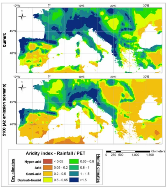
(2071-2100, A2 emission scenario), using the UNEP aridity index (UNEP, 1997); the current map is based on the climate data by New et al. (2002), while the climate change map is based on results from the HADRM3 RCM (PRUDENCE, 2007). ...15 Figure 2.3 – Characteristic time-length combinations of climatic and hydrological processes, adapted from

Blöschl and Sivapalan (1995), with inter-annual climate cycles and climate changes added over original picture; scale denominators indicate typical working and modeling scales...18 Figure 2.4 – Theoretical framework for vulnerability assessment, adapted from Gallopín (2006) with items

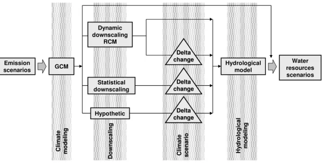
relevant to this thesis in italic...35 Figure 2.5 – Schematic representation of methods to assess the impacts of climate change on water resources

(adapted from Xu and Singh, 2004)...48 Figure 2.6 – Climate change estimates for central and south Portugal for 2071-2100 considering the A2 and B2

emission scenarios, resulting from 3 GCM estimates downscaled using 13 different RCMs to a resolution of 50×50 Km; model results were obtained in the PRUDENCE project (PRUDENCE, 2007)...63 Figure 3.1 – Framework for vulnerability assessment, adapted from Gallopín (2006), superimposed over the

modeling framework...84 Figure 3.2 – Framework for a multi-scale analysis of the sensitivity of hydrological, vegetation and erosion

processes to climate changes...85 Figure 3.3 – Framework used for a multi-scale analysis of the resilience of hydrological, vegetation and erosion

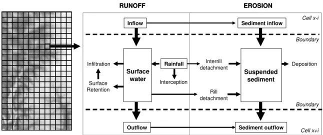
processes to RCM-based climate change scenarios. ...87 Figure 3.4 – Spatial distribution approach used by MEFIDIS: 1. division of target watershed into a matrix of

orthogonal grid cells, 2. computation of runoff generation and detachment for each grid cell, 3. routing overland flow and suspended sediment following the steepest slope. ...91 Figure 3.5 – Processes simulated by the model within each cell and at the boundaries between grid cells.91 Figure 3.6 – Average runoff and erosion estimates for the different sensitivity tests, expressed as test average

divided by the overall average for all tests, for the patch scale (top) and field/hillslope scale (bottom). ...102 Figure 3.7 – Correlation coefficient between runoff and soil moisture, depth and porosity, for the different

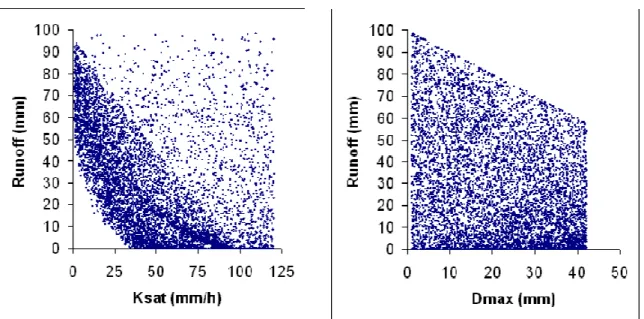
sensitivity tests at the patch scale (top) and field/hillslope scale (bottom). ...104 Figure 3.8 – Runoff estimates per saturated hydraulic conductivity (left) and depression storage capacity (right)

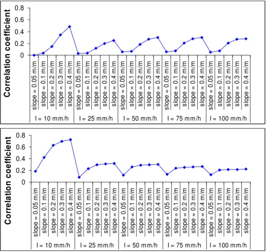
for the hillslope/field scale test, 100 mm.h-1 rainfall intensity and 0.4 m.m-1 slope...105 Figure 3.9 – Correlation coefficient between erosion and runoff, for the different sensitivity tests at the patch

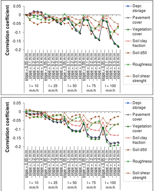
scale (top) and field/hillslope scale (bottom). ...106 Figure 3.10 – Correlation coefficient between erosion and model landcover and soil parameters, for the different

sensitivity tests at the patch scale (top) and field/hillslope scale (bottom). ...107 Figure 3.11 – The Lucky Hills 103 (top) and Ganspoel (bottom) catchments, with 5 m contour lines; darker lines

(16)

Figure 3.12 – Measured and simulated results for net erosion in Ganspoel and Lucky Hills 103, compared with the 1:1 agreement line (logarithmic scale). ...115 Figure 3.13 – Relationship between erosion magnitude and relative difference between measured and simulated

values (the error divided by the sum of measured and simulated values). ...116 Figure 3.14 – Comparison of simulated and measured net erosion in Ganspoel, with MEFIDIS using a standard

calibration for all storms and a unique calibration per storm. ...117 Figure 3.15 – Simulated (top) and observed (bottom) patterns of erosion (grey) and deposition (black) in

Ganspoel, for May 1997; lines represent field boundaries. ...119 Figure 3.16 – Variation of average simulated erosion and deposition rates with distance to observed erosion and

deposition features in Ganspoel, for May 1997...120 Figure 3.17 – Sensitivities of model runoff predictions relative to changes in inputs for the Ganspoel watershed,

for the tests described in Table 3.9, with the dotted lines showing the median of model sensitivities and CV representing the coefficients of variation. ...126 Figure 3.18 – Sensitivities of model runoff predictions relative to changes in inputs for the Lucky Hills 103

watershed, for the tests described in Table 3.9, with the dotted lines showing the median of model sensitivities and CV representing the coefficients of variation. ...126 Figure 3.19 – Sensitivities of model sediment yield predictions relative to changes in inputs for the Ganspoel

watershed, for the tests described in Table 3.9, with the dotted lines showing the median of model sensitivities and CV representing the coefficients of variation. ...127 Figure 3.20 – Sensitivities of model sediment yield predictions relative to changes in inputs for the Lucky Hills

103 watershed, for the tests described in Table 3.9, with the dotted lines showing the median of model sensitivities and CV representing the coefficients of variation. ...127 Figure 4.1 – Map of Portugal showing the location of the study areas superimposed over the climate aridity index

(UNEP, 1997), calculated using the spatial datasets for long-term average rainfall and potential evapotranspirations available in SNIRH (2006)...140 Figure 4.2 – Guadiana study area, showing major rivers and the Odeleite watershed (in red)...142 Figure 4.3 – Tejo study area, showing major rivers and the Alenquer watershed (in red). ...143 Figure 4.4 – Meteorological sampling network in the Guadiana (left) and Tejo (right) study areas; station codes

follow the SNIRH system for classification except when beginning by IM, in which case they refer to stations operating by the Portuguese Meteorological Institute...145 Figure 4.5 – 1961-1990 climate normals for rainfall and temperature for climate stations in the Guadiana (top)

and Tejo (bottom); location is shown in Figure 4.4. ...146 Figure 4.6 – Annual rainfall and mean temperature for the Guadiana (left) and Tejo (right), for the hydrological

years from 1976/77 to 1989/90 (SNIRH, 2006); horizontal lines represent average rainfall (blue) and temperature (red) for the sampling period...147 Figure 4.7 – Cumulative histogram for the distribution of monthly (left) and daily (right) rainfall in both study

areas, for the period from 1976/77 to 1989/90 (SNIRH, 2006)...147 Figure 4.8 – Comparison between selected storms and Intensity-Duration-Frequency (IDF) curves for the Odeleite (left) and Alenquer (right) watersheds, determined by Brandão et al. (2001). ...149 Figure 4.9 – Hydrometric and sediment sampling network in the Guadiana (left) and Tejo (right) study areas;

(17)

Figure 4.10 – Comparison between sediment-discharge measurements (SNIRH, 2006) and sediment rating curves for the Odeleite (left) and Alenquer (right) watersheds, in logarithmic scale...152 Figure 4.11 – Average monthly estimates for rainfall and runoff in the Guadiana (left) and Tejo (right) study

areas, using data from the stations shown in Table 4.5 and Table 4.4 (SNIRH, 2006)...155 Figure 4.12 – Annual estimates for rainfall subsurface and surface runoff in the Guadiana (left) and Tejo (right)

study areas, using data from the stations shown in Table 4.4 and Table 4.5 for the hydrological years from 1976/77 to 1989/90 (SNIRH, 2006); the horizontal blue lines show the average annual runoff within this period. ...156 Figure 4.13 – Relationship between rainfall and surface runoff for the Odeleite (top) and Alenquer (bottom)

watersheds, for the storms represented in Table 4.6 and Table 4.7 respectively; symbol size represents the storm baseflow in proportion to the average baseflow for the entire dataset. ...159 Figure 4.14 – Topography for the Guadiana (left) and Tejo (right) study areas; the dataset was produced by

Jarvis et al. (2006) from the SRTM 90×90 m DEM, and cut using watershed limits. ...161 Figure 4.15 – Comparison between observed channel width and drained area for points within the Odeleite and

Alenquer catchments (and in catchments neighboring Odeleite)...162 Figure 4.16 – Topographic wetness index distribution for Odeleite (left) and Alenquer (right), calculated

following equation 3.17. ...163 Figure 4.17 – Measured daily recession curves after 3 storms for Odeleite and Alenquer. ...164 Figure 4.18 – Soil types in the Guadiana (left) and Tejo (right) study areas, classified according to the 1990 FAO

soil classification (Driessen et al., 2001), following the 1978 1:1,000,000 FAO soil map (Cardoso et al., 1973). ...166 Figure 4.19 – Soil types in the Odeleite (left) and Alenquer (right) watersheds, classified according to the 1990

FAO soil classification (Driessen et al., 2001), following the 1:50,000 DGADR soil map (Gonçalves et al., 2005). ...172 Figure 4.20 – Land cover in the Guadiana (left) and Tejo (right) study areas, from the 1:100,000 1990 CORINE

Land Cover map (EEA, 1995). ...176 Figure 4.21– Land cover in the Odeleite (left) and Alenquer (right) watersheds, obtained using remote sensing

data...181 Figure 4.22 – Runoff and erosion results from the rainfall simulation experiments performed in Portel (left) and

Alenquer (right). ...185 Figure 4.23 – Location of meteorological and river sampling stations in the study areas; the upper left corner

shows the UNEP aridity index (UNEP, 1992) for Portugal, calculated using the data provided via SNIRH (2006), while the inserts show the sampling stations for the Guadiana (a) and Tejo (b) areas used for SWAT evaluation. ...189 Figure 4.24 – Observed and simulated average annual river flow in the Guadiana (a; r2_{= 0.86, p < 0.01) and Tejo}

(b; r2_{= 0.83, p < 0.01) catchments...191} Figure 4.25 – Observed and simulated annual sediment yield in the Guadiana (a; r2 = 0.93, p < 0.01) and Tejo (b;

r2 = 0.76, p < 0.01) catchments. ...193 Figure 4.26 – Observed and simulated average monthly river flow in the Guadiana (a; r2 = 0.76, p < 0.01) and

(18)

Figure 4.27 – Observed and simulated monthly sediment yield per unit area in the Guadiana (a; r2_{= 0.78, p <} 0.01) and Tejo (b; r2_{= 0.58, p < 0.01) catchments (square root of values). ...198} Figure 4.28 – Observed and simulated runoff (left) and soil erosion (right) for the rainfall simulation experiments

in Portel. ...205 Figure 4.29 – Observed and simulated runoff (left) and soil erosion (right) for the rainfall simulation experiments

in Alenquer...206 Figure 4.30 – Observed and simulated runoff at the catchment outlet for Odeleite (a, left) and Alenquer (b, right).

...209 Figure 4.31 – Observed and simulated peak runoff rate at the catchment outlet for Odeleite (a, left) and Alenquer

(b, right). ...211 Figure 4.32 – Observed and estimated catchment sediment yield for Odeleite (a, left) and Alenquer (b, right).

...212 Figure 4.33 – Schematic representation (side view) of soil flume and the nozzles; storm movement was obtained

by moving the support structure of the rainfall simulator at a constant speed, with surface runoff collected at the end of the flume...218 Figure 4.34 – Numerical simulation (continuous line) and observed (laboratory data measured in soil flume)

runoff hydrographs (left) and accumulated sediment loss (right) for downstream and upstream moving storms, for a storm with 0.12 m/s speed, and rainfall intensity of c. 4 mm/h...219 Figure 4.35 – Spatial extent of test storms (0.5, 1 and 2 times the basin axial length). Circumferences in the

upper left and lower right show the beginning and the end of storm movement over the basin axis which is represented by the diagonal line...220 Figure 4.36 – Frequency of test storms; IDF curves for S. Julião do Tojal, near Alenquer, determined by Brandão

et al. (2001), where P is the return period. ...221 Figure 4.37 – Relative difference between the results for upstream and downstream storm movements shown in

Table 4.47; positive values indicate that the results increase with downstream movement. ...223 Figure 4.38 – Simulated hydrographs for several sections in the Alenquer river (right) and its tributaries (left) for

test Medium/Medium, for both downstream and upstream storm movements (see also Table 4.46).225 Figure 4.39 – Left: simulated hydrographs at the Alenquer basin’s outlet for tests Medium/Fast (left),

Medium/Medium (center) and Medium/Slow (right), for both downstream and upstream movements (see Table 4.46); Right: simulated peak runoff rate at the Alenquer basin’s outlet as a function of storm intensity, for all 18 tests. ...225 Figure 4.40 – Left: Sediment Yield Ratio (net erosion / gross erosion) for downstream and upstream storm

movements (see Table 4.46); right: net erosion increase with downstream storm movement, in the Alenquer basin, for all 18 tests, correlated with the increase in peak runoff rates (above) and total runoff (below), with the arrow in the upper figure indicating the position of one outlier...226 Figure 5.1 – Roadmap for the results shown in this chapter, following the vulnerability analysis framework

described in section 3.1. ...237 Figure 5.2 – Relation between climate change scenarios for temperature and rainfall, for central and southern

(19)

Figure 5.3 – Simulated responses of evapotranspiration, surface runoff and subsurface runoff to changes in temperature (T – left), rainfall (PP – center) and atmospheric CO2 concentration (CO2 – right) for the Guadiana (a) and the Tejo (b). ...242 Figure 5.4 – Simulated responses of evapotranspiration, surface runoff and subsurface runoff to changes in

rainfall, considering constant rainfall intensity (PI – left), intensity decreasing at half the decrease in rainfall rate (PM – center), and intensity decreasing at the same rate as rainfall (PD – right) for the Guadiana (a) and Tejo (b) watersheds. ...243 Figure 5.5 – Simulated responses of total biomass growth and soil erosion of different vegetation covers to

changes in temperature (T – left), rainfall (PP – center) and atmospheric CO2 concentration (CO2 – right) for the Guadiana (a) and Tejo (b) watersheds; the vegetation cover types are cork oaks, mediterranean shrubs and wheat for the Guadiana, and pine forest, vines and wheat for the Tejo. ...244 Figure 5.6 – Simulated responses of evapotranspiration, surface runoff and subsurface runoff to the combined

changes in climate described in Table 5.2 for the Guadiana (a) and the Tejo (b), with the “low rainfall” test on the left and the “high rainfall” on the right. ...249 Figure 5.7 – Simulated responses of total biomass growth and erosion of different vegetation covers to the

combined changes in climate described in Table 7 for the Guadiana (a) and Tejo (b) watersheds; the vegetation cover types are cork oaks, mediterranean shrubs and wheat for the Guadiana, and pine forest, vines and wheat for the Tejo...251 Figure 5.8 – Impact of biomass changes on canopy cover and interception storage for the most important

vegetation types in the Alenquer and Odeleite watersheds. ...257 Figure 5.9 – Averaged changes to runoff and peak runoff rates in both study areas for changes to rainfall (left),

soil water deficit (center) and land cover (right); test designations are explained in Table 5.4. ...262 Figure 5.10 – Current and changed runoff generation per storm, for Odeleite (a) and Alenquer (b), for test Ich0.5,

PPch (as defined in Table 5.4). ...263 Figure 5.11 – Averaged changes to sediment yield in both study areas for changes to rainfall (left), soil water

deficit (center) and land cover (right); test designations are explained in Table 5.4...264 Figure 5.12 – Sensitivity to change (in % per % change) of runoff to changes to rainfall, soil water deficit and

land cover, per storm, for Odeleite (a) and Alenquer (b); test designations are explained in Table 5.4. ...264 Figure 5.13 – Sensitivity to change (in % per % change) of peak runoff rate to changes to rainfall, soil water

deficit and land cover, per storm, for Odeleite (a) and Alenquer (b); test designations are explained in Table 5.4. ...265 Figure 5.14 – Sensitivity to change (in % per % change) of sediment yield to changes to rainfall, soil water

deficit and land cover, per storm, for Odeleite (a) and Alenquer (b); test designations are explained in Table 5.4. ...265 Figure 5.15 – Averaged changes to upslope erosion and sediment delivery ratio in both study areas for changes

to rainfall (left), soil water deficit (center) and land cover (right); test designations are explained in Table 5.4. ...268 Figure 5.16 – Averaged changes to erosion in areas with significant erosion rates and to catchment area suffering

(20)

land cover (right); significant erosion rate is defined as being above 1 ton.ha-1_{, and test designations are} explained in Table 5.4. ...269 Figure 5.17 – Comparison between PROMES results and measured values for monthly maximum and minimum

temperatures in the Guadiana (a, left) and the Tejo (b, right) study areas; climate stations are identified in Figure 4.5. ...272 Figure 5.18 – Comparison between PROMES results and measured values for monthly rainfall in the Guadiana

(a, left) and the Tejo (b, right) study areas; climate stations are identified in Figure 4.5...273 Figure 5.19 – Map of Portugal showing the location of the study areas superimposed over the climate aridity

index (UNEP, 1997), for current conditions (left), the A2 PROMES scenario (center) and the B2 scenario (right); the Guadiana area is located in southeastern Portugal, while the Tejo area is located in the west. ...275 Figure 5.20 – PROMES results for the control conditions (1961-90) and climate change scenarios A2 and B2

(2071-2100) showing the cumulative histogram for average annual temperature in the Guadiana (a, left) and Tejo (b, right) study areas...276 Figure 5.21 – PROMES results for the control conditions (1961-90) and climate change scenarios A2 and B2

(2071-2100) showing the cumulative histogram for annual rainfall in the Guadiana (a, left) and Tejo (b, right) study areas. ...276 Figure 5.22 – PROMES results for the control conditions (1961-90) and climate change scenarios A2 and B2

(2071-2100) showing the cumulative histogram for annual aridity in the Guadiana (a, left) and Tejo (b, right) study areas; aridity is measured using the aridity index developed by UNEP (1997)...278 Figure 5.23 – PROMES results for average monthly maximum and minimum temperature in the control situation

(1961-90) and climate change scenarios A2 and B2 (2071-2100), for the Guadiana (a, left) and Tejo (b, right) study areas. ...279 Figure 5.24 – PROMES results for average monthly rainfall in the control situation (1961-90) and climate

change scenarios A2 and B2 (2071-2100), for the Guadiana (a, left) and Tejo (b, right) study areas.279 Figure 5.25 – PROMES results for average daily rainfall in storm days (with rainfall above 10 mm), for the OND

and JFMA seasons, in the control situation (1961-90) and climate change scenarios A2 and B2 (2071-2100), for the Guadiana (a, left) and Tejo (b, right) study areas; the black lines represent the standard deviation between years. ...281 Figure 5.26 – SWAT results for the control run (1961-90) and climate change scenarios A2 and B2 (2071-2100),

using the PROMES A2 and B2 scenarios shown in Table 5.8, showing the cumulative histogram for annual runoff in the Guadiana (a) and Tejo (b) study areas. ...283 Figure 5.27 – SWAT results for average monthly surface runoff (Qsurf) and subsurface runoff (Qsub) in the

control conditions (top, 1961-90) and climate change scenarios A2 (center, 2071-2100) and B2 (bottom, 2071-2100), using the PROMES A2 and B2 scenarios shown in Table 5.8, for the Guadiana (a, left) and Tejo (b, right) study areas. ...284 Figure 5.28 – SWAT results for average annual biomass growth for wheat (top), cork oak and forest (center) and

(21)

Figure 5.29 – Changes to the Manning’s n, canopy cover and interception storage of different vegetation types in the Guadiana (left) and Tejo (right) study areas, calculated from the SWAT results for biomass changes for the PROMES A2 and B2 climate change scenarios...291 Figure 5.30 – Current and changed runoff (top) and peak runoff rates (bottom) in the Odeleite (a, left) and Alenquer (b, right) watersheds, for the scenarios described in Table 5.17. ...294 Figure 5.31 – Current and changed runoff generation ratio in the Odeleite (a, left) and Alenquer (b, right)

watersheds, for the scenarios described in Table 5.17. ...295 Figure 5.32 – Current and changed sediment yield (top) and upslope erosion (bottom) in the Odeleite (a, left) and

Alenquer (b, right) watersheds, for the scenarios described in Table 5.17. ...298 Figure 5.33 – Relationship between catchment area and total erosion in regions with significant erosion rates, in

the Odeleite (a, left) and Alenquer (b, right) watersheds; significant erosion rate is defined as being above 1 ton.ha-1_{, and the scenarios are described in Table 5.17...300} Figure 6.1 – Relation between changes to temperature and rainfall for the low and high rainfall simulations used

in the sensitivity analysis (section 5.1), the PROMES RCM climate change scenarios (section 5.3), and published scenarios for central and southern Portugal (Cunha et al., 2002; PRUDENCE, 2007;

approximated CO2 concentrations). ...313 Figure 6.2 – Estimated relationship between soil fertility loss due to erosion and depth to bedrock, following the

thresholds and curve shapes proposed by Bakker et al. (2004), with the range of soil depth and fertility loss estimates for the Guadiana study area superimposed...318 Figure 6.3 – Impacts of climate change and soil erosion on wheat productivity for the climate change scenarios

used in the sensitivity analysis (section 5.1) for the Guadiana lithosols (a) and Tejo (b) study areas.319 Figure 6.4 – Current and estimated runoff per inhabitant for the Guadiana (a) and Tejo (b) basins, under the

climate change scenarios presented in section 5.1 and shown in Figure 6.1; horizontal lines indicate the stress thresholds shown in Table 6.2...327 Figure 6.5 – Current and estimated runoff per inhabitant for the Guadiana (a) and Tejo (b) basins, under the

climate change scenarios presented in section 5.3 and shown in Figure 6.1, for average and drought conditions; horizontal lines indicate the stress thresholds shown in Table 6.2. ...329 Figure 6.6 – Agriculture and natural vegetation distribution in the Guadiana study area broken down by climatic

aridity classes (UNEP, 1997)...333 Figure 6.7 – Comparison between changes to aridity for the climate change scenarios shown in Figure 6.1 and

the vegetation thresholds shown in Table 6.5, for the Guadiana (a) and Tejo (b) study areas...336 Figure 6.8 – Agriculture and natural vegetation distribution in the Guadiana study area over different soil types,

broken down by climatic aridity classes (UNEP, 1997). ...342 Figure 6.9 – Relation between changes to temperature and rainfall for the vulnerability assessment scenarios

(22)

Index of Tables

Table 2.1 – Description and predicted atmospheric CO2 concentrations for the SRES emission scenarios and the antecedent IS92 scenarios, based on the SRES report (IPCC, 2001); concentrations in 2000 were estimated at c. 370 ppm. ...13 Table 2.2 – Spatial controls on surface and subsurface flow at multiple scales, with characteristic lengths similar

to those shown in Figure 2.3. ...20 Table 2.3 - Temporal controls on catchment flow at multiple scales, with characteristic times similar to those

shown in Figure 2.3...21 Table 2.4 – Characteristic time-length combinations of erosive processes, adapted from Favis-Mortlock et al.

(2001) and Imeson and Lavee (1998); sample processes are taken from Imeson and Lavee (1998).26 Table 2.5 – Characteristic spatial scales of erosion and sedimentation processes, associated with erosion,

transport or deposition dominance, with characteristic lengths similar to those shown in Figure 2.3.27 Table 2.6 – Spatial constraints on erosion processes at multiple scales, following Lane et al. (1997), with

characteristic lengths similar to those shown in Figure 2.3...29 Table 2.7 – Temporal constraints on erosion processes at multiple scales, with characteristic times similar to

those shown in Figure 2.3. ...30 Table 2.8 – Representative sample of current hydrological-erosion models. ...42 Table 2.9 – Mismatch between the capabilities of current GCMs and hydrological assessment requirements

(adapted from Xu and Singh, 2004). ...47 Table 2.10 – Comparison between estimated climate change impacts on hydrological processes and existing

impact assessment studies. ...64 Table 2.11 – Comparison between estimated climate change impacts on soil erosion processes and existing

impact assessment studies. ...65 Table 3.1 – Spatially-distributed parameters required by MEFIDIS. ...98 Table 3.2 - Results provided by MEFIDIS as time-series for the entire watershed. ...100 Table 3.3 – Parameter range used in the MEFIDIS sensitivity analysis. ...101 Table 3.4 – Characteristics of events used in the model evaluation exercise. ...111 Table 3.5 – Calibrated hydraulic conductivity and depression storage capacity compared with measured values.

...112 Table 3.6 – Measured and simulated results for the events detailed in Table 3.4...114 Table 3.7 – Overall correlation coefficient, Nash-Sutcliffe efficiency index and average unsigned error for the

results shown in Table 3.6...115 Table 3.8 – Measured and simulated results for the events detailed in Table 3.4, for Lucky Hills 101. ..118 Table 3.9 – Characteristics of the rainfall and vegetation cover change tests...124 Table 4.1 – Characteristics for the selected storms in the Odeleite watershed, calculated from data collected via

SNIRH (2006). ...148 Table 4.2 – Characteristics for the selected storms in the Alenquer watershed, calculated from udographs

(23)

Table 4.3 – Sediment rating curve (equation 4.1) parameters for sampling stations in the Guadiana and Tejo study areas, together with range of application, number of samples, correlation coefficient and level of significance, calculated using data from SNIRH (2006)...152 Table 4.4 – Sampling period, drained area and hydrological and sediment yield characteristics for watersheds in

the Guadiana study area (SNIRH, 2006)...153 Table 4.5 – Sampling period, drained area and hydrological and sediment yield characteristics for watersheds in

the Tejo study area (SNIRH, 2006). ...154 Table 4.6 – Hydrological characteristics and sediment yield for the selected storms in the Odeleite watershed,

calculated from data collected via SNIRH (2006). ...157 Table 4.7 – Hydrological characteristics and sediment yield for the selected storms in the Alenquer watershed,

calculated from hydrographs supplied by INAG. ...158 Table 4.8 – Main soil types shown in Figure 4.18 and physical properties for the entire profile, following Batjes

(2002)...167 Table 4.9 – Soil physical and hydraulic parameters for the surface layer (Batjes, 2002)...168 Table 4.10 – Soil physical and hydraulic parameters for the subsurface layer (Batjes, 2002). ...168 Table 4.11 – Soil texture parameters for the surface layer (Batjes, 2002)...169 Table 4.12 – Soil texture parameters for the subsurface layer (Batjes, 2002). ...169 Table 4.13 – Correspondence between the 1990 FAO soil classification (Driessen et al., 2001) and the

Portuguese soil classification, used by DGADR (Cardoso, 1965), for soils occurring in the Odeleite and Alenquer watersheds, according to Pimenta (1998); the DGADR soil sample data used to extract physical soil parameters for each soil patch is also shown...171 Table 4.14 – Soil hydraulic and texture parameters for the Odeleite watershed, showing median values followed

by parameter range where multiple samples are present; parameters are identified in Table 3.1. ..172 Table 4.15 – Soil hydraulic and texture parameters for the Alenquer watershed, showing median values followed

by parameter range where multiple samples are present; parameters are identified in Table 3.1. ..173 Table 4.16 – Correspondence table between CLC classes and the land cover classes used by the SWAT model,

for vegetated land covers. ...175 Table 4.17 – Land cover types not present in the SWAT database, and the vegetation species used to

parameterize the land cover type. ...177 Table 4.18 – Radiation-use efficiency and phenology parameters for Mediterranean vegetation; references are

shown in Table 4.22...177 Table 4.19 – Parameters for Mediterranean vegetation physical characteristics, response to temperature and

biomass nutrient content; references are shown in Table 4.22...178 Table 4.20 – Parameters for Mediterranean vegetation response to vapor pressure deficit and atmospheric CO2

concentration; references are shown in Table 4.22. ...178 Table 4.21 – Other Mediterranean vegetation parameters; references are shown in Table 4.22. ...179 Table 4.22 – References for SWAT land cover parameters for Mediterranean vegetation. ...179 Table 4.23 – Average annual dry weight yield for major crops in the Guadiana and Tejo study areas, averaged

(24)

Table 4.24 – Land use parameters for the Odeleite and Alenquer watersheds, showing the most common values followed by parameter range where multiple samples are present; parameters are identified in Table 3.1. ...182 Table 4.25 – Average annual observations for soil erosion in the Vale Formoso center for different agricultural

land use types, after 22 years of observations, following Tomás and Coutinho (1993)...183 Table 4.26 – Comparison between the scales used in the SWAT model application for different parameters with

the appropriate scales determined by Booij (2003). ...187 Table 4.27 – Calibration and validation statistics for mean annual river flow...190 Table 4.28 – Calibration and validation statistics for mean annual sediment yield. ...192 Table 4.29 – Observed (INE, 2006) and predicted results for average annual yields for the major crops in the two

study areas...193 Table 4.30 – Observed and simulated results for average annual erosion rates for the most important land cover

types in the two study areas; observed average and range are taken from standard plot measurements in several northern Mediterranean regions from the review published by Poesen and Hooke (1997) and Wainwright and Thornes (2004). ...194 Table 4.31 – Calibration and validation statistics for mean monthly river flow...195 Table 4.32 – Calibration and validation statistics for monthly sediment yield. ...197 Table 4.33 – Model performance statistics for monthly river flow and sediment export, for selected sampling

stations in the Guadiana study area. ...199 Table 4.34 – Model performance statistics for monthly river flow and sediment export, for selected sampling

stations in the Tejo study area. ...199 Table 4.35 – Model performance statistics for average monthly river flow and sediment yield when using a

stochastic weather generator. ...201 Table 4.36 – Observed and predicted results for average annual yields for the major crops in the two study areas

when using a stochastic weather generator. ...201 Table 4.37 – Model calibration statistics for the rainfall simulation experiments. ...205 Table 4.38 – Calibrated soil hydraulic and texture parameters for the Odeleite and Alenquer watersheds;

parameters are identified in Table 3.1. ...207 Table 4.39 – Calibrated land use parameters for the Odeleite and Alenquer watersheds; parameters are identified

in Table 3.1. ...207 Table 4.40 – Calibration and validation statistics for total storm runoff. ...208 Table 4.41 – Calibration and validation statistics for peak runoff rate. ...210 Table 4.42 – Calibration and validation statistics for time to hydrograph peak...210 Table 4.43 – Calibration and validation statistics for sediment yield. ...212 Table 4.44 – Comparison between estimated and simulated sediment delivery ratio and ephemeral gully to rill /

interill erosion ratio for Odeleite and Alenquer. ...213 Table 4.45 – Comparison between model results for sediment sources (in terms of fraction of total upslope

erosion) for each landcover in both study areas, and their distribution over the catchments. ...214 Table 4.46 – Characteristics of the 9 test storms simulated for the Alenquer drainage basin study. ...220 Table 4.47 – Summary of all simulation results for all tests conducted in the Alenquer drainage basin; runoff and

(25)

Table 5.1 – Response of evapotranspiration, surface runoff and subsurface runoff to changes in climatic parameters, in mm per year...241 Table 5.2 – Characteristics of simulation sets to explore the consequences of combined changes in climate

parameters; changes are shown as percentage over current average annual values. ...248 Table 5.3 – Response of evapotranspiration, surface runoff and subsurface runoff to changes in multiple climatic

parameters, in mm per year...249 Table 5.4 – Approach used in the sensitivity analysis, describing the different variables and tests...257 Table 5.5 – Average sensitivity to change (in % per % change) of runoff, peak runoff rate and sediment yield for

both study areas, for the tests described in Table 5.4...259 Table 5.6 – Average sensitivity to change (in % per % change) of upslope erosion, sediment delivery ratio, and

both total erosion and catchment area in regions with significant erosion rates, for both study areas; significant erosion rate is defined as being above 1 ton.ha-1_{, and the tests are described in Table 5.4.267} Table 5.7 – Average correction applied to the PROMES climate parameters in both study areas, and the

correlation between the uncorrected climate model results and observations...273 Table 5.8 – Predicted average annual changes in climate parameters for the PROMES A2 and B2 scenarios,

compared with the control run. ...274 Table 5.9 – Lower and upper percentile annual temperature values, measured in ºC above or below long-term

annual average, for the PROMES control, A2 and B2 scenarios...277 Table 5.10 – Lower and upper percentile rainfall values, measured in % above or below long-term annual average, for the PROMES control, A2 and B2 scenarios. ...277 Table 5.11 - Percentage of annual rainfall falling on each season for the PROMES control, A2 and B2 scenarios;

SON is September, October and November, DJF is December, January and February, MAM is March, April and May, and JJA is June, July and August...280 Table 5.12 – SWAT results for average annual changes in hydrological parameters, in comparison with a control

run, using the PROMES A2 and B2 scenarios shown in Table 5.8. ...282 Table 5.13 – SWAT results for lower and upper percentile annual runoff values, measured in % above or below

long-term average, using the PROMES control, A2 and B2 scenarios...283 Table 5.14 – SWAT results for average annual changes in vegetation biomass growth, using the PROMES A2

and B2 scenarios shown in Table 5.8...285 Table 5.15 – SWAT results for lower and upper extreme biomass production values in the Guadiana, measured

in % above or below long-term annual average, using the PROMES control, A2 and B2 scenarios.288 Table 5.16 – SWAT results for lower and upper extreme biomass production values in the Tejo, measured in %

above or below long-term annual average, using the PROMES control, A2 and B2 scenarios...288 Table 5.17 – SWAT results for average changes in subsurface runoff during the OND and JFMA seasons, using

the PROMES A2 and B2 scenarios shown in Table 5.8, compared with the changes in storm rainfall shown in Figure 5.25...289 Table 5.18 – Impacts of changes to subsurface runoff (shown in Table 5.17) on soil water deficit during the OND

and JFMA seasons, using the PROMES A2 and B2 scenarios, for the Odeleite and Alenquer study areas. ...290 Table 5.19 – Average change (in %) of runoff and peak runoff rate for both study areas, for the scenarios

(26)

Table 5.20 – Average change (in %) of sediment yield, upslope erosion and sediment delivery ratio for both study areas, for the scenarios described in Table 5.17. ...296 Table 5.21 – Average change (in %) of upslope erosion under different land uses for both study areas, for the

scenarios described in Table 5.17...299 Table 5.22 – Average change (in %) of total erosion and catchment area in regions with significant erosion rates,

for both study areas; significant erosion rate is defined as being above 1 ton.ha-1, and the scenarios are described in Table 5.17. ...300 Table 6.1 – Impacts of climate change and soil erosion on wheat productivity for the PROMES climate change

scenarios described in section 5.3; the Guadiana results refers to lithosols. ...318 Table 6.2 – Water stress thresholds, following Arnell (2004). ...323 Table 6.3 – Annual average water availability and consumption for the Guadiana and Tejo river basins (INAG,

1999a and b)...324 Table 6.4 – Current and estimated runoff changes and water withdrawal ratios for the climate change scenarios

presented in section 5 and shown in Figure 6.1; for withdrawal ratios, numbers in bold indicate severe water stress, while underline numbers indicate water shortfalls (withdrawals above runoff rates).326 Table 6.5 – Estimated aridity thresholds for different vegetation types in the study areas, compared with other

dryland estimates...335 Table 6.6 – Estimated optimal canopy conductance and changes to maximum potential LAI for the Guadiana and

Tejo study areas, for the climate change scenarios shown in Figure 6.1...339 Table 6.7 – Climate change scenarios used for vulnerability assessment...345 Table 6.8 – Frequency of occurrence of each climate change scenario (Figure 6.9) within each vulnerability

assessment scenario (Table 6.7); CO2 concentration values are approximate...346 Table 6.9 – Main vulnerabilities of the Guadiana and Tejo study areas to climate change, in terms of impacts on

hydrological processes, vegetation productivity and soil erosion capable of enhancing desertification. ...347 Table 6.10 – Current and estimated water withdrawal ratios for the vulnerability scenarios described in Table

(27)

1. Introduction

There is a growing consensus in Earth systems sciences that global temperatures are increasing and will continue during the next century, leading to changes in global climate patterns (IPCC, 2007). Different regions of the globe are expected to respond differently to global warming; the Mediterranean region has been identified as one of the Earth’s primary “hot-spots” for climate change, due to the magnitude of expected changes to temperature and rainfall patterns (Giorgi, 2006), associated with an increase in extreme episodes such as heat waves and high-intensity storms (Räisänen et al., 2004).

The expected impacts of climate change on Mediterranean regions point to a trend of increased vulnerability of both natural and human systems due to the reduction of available water resources and increased land degradation (Schroter et al., 2005). This trend is expected to accelerate the process of desertification already occurring in these regions (Puigdefábregas, 1998). There is a need to quantify the impacts of climate change on the most important physical drivers of desertification – water resources, soil erosion and vegetation productivity – to estimate impacts and support the development of adequate adaptation measures (Huntingford et al., 2006).

These issues have been partly addressed in recent years, thanks to a significant research effort focusing on the regional impacts of climate change on hydrology (e.g. Xu and Singh, 2004) and vegetation productivity (e.g. Field et al., 2007). Research on the impacts on soil erosion has been more limited, although some work has been performed for North American regions (e.g. Nearing et al., 2004). However, these efforts have been conditioned by the large spatial and temporal scales at which climate change predictions are typically made, limiting impact studies for meso-scale and smaller watersheds, within-catchment dynamics, and temporal anomalies such as extreme floods and droughts (Bronstert, 2004). These problems have also significantly limited research on the impacts of climate change on soil erosion, due to the high variability in time and space of erosive processes (Michael et al., 2005).

(28)

regions therefore requires an analysis at multiple spatial and temporal scales, ranging from slope to catchment and taking localized storms into account, as issue which has been neglected in the recent literature (Imeson and Lavee, 1998; Boardman, 2006).

This thesis aims to take a further step towards analyzing and quantifying the impacts of climate change on the physical drivers for desertification processes in Mediterranean watersheds at multiple spatial and temporal scales, focusing on meso-scale catchments (c. 100 to 1000 Km2). The main objective of this thesis is to assess the vulnerability of hydrological, soil erosion and vegetation productivity patterns in Mediterranean

watersheds to climate change, resulting from enhanced biophysical desertification

processes.

To achieve this goal, a vulnerability analysis framework is followed which focuses on: (i) the sensitivity of hydrological, vegetation and erosive patterns to changes in climate, (ii) the magnitude of the expected impacts, and (iii) the main biophysical components requiring adaptation, following the concepts exposed by Adger (2006). The analysis estimates seasonal, annual and long-term trends at the watershed scale, and uses these trends as boundary conditions to evaluate changes in within-catchment processes during extreme rainfall events in higher spatial and temporal detail. This allows an evaluation of the processes linking climate, hydrology, soil erosion and vegetation productivity operating at different spatial and temporal scales, taking into account cross-scale interactions.

This thesis is supported by a multi-scale modeling framework, using a seasonal-scale model to analyze long-term watershed trends and integrating these results into spatially detailed simulations at the extreme events scale. Models are currently the most appropriate tools to support climate change studies since they codify the existing knowledge on catchment processes and their response to meteorological forcing, allowing the quantification of the impacts of changed climate patterns in a feasible way (Bronstert, 2004).

The thesis is organized in 7 chapters, as follows:

Chapter 2 provides the conceptual background for this thesis. It begins with an overview of

(29)

focusing on modeling tools; the current status of climate change impact assessment is then discussed, and the most important research gaps are identified.

Chapter 3 describes the main objectives of this thesis as well as the methodology used to

achieve them. The methodological framework is based on a multi-scale, model-based vulnerability assessment, beginning with an analysis of the sensitivity of hydrological, vegetation and erosive processes to different degrees of change in climate parameters at multiple scales, followed by a cross-scale assessment of the resilience of these processes by analyzing the impacts of two climate change scenarios. The chapter then proceeds to present the modeling tools used in the two analysis scales. The spatially detailed, extreme event erosion model MEFIDIS – Physically-based Distributed Erosion Model (Modelo de Erosão FÍsico e DIStribuído – Nunes et al., 2006), optimized for Mediterranean watersheds, is developed within this thesis. MEFIDIS is evaluated using two well studied watersheds, and its sensitivity to changes in climate parameters is compared with other erosion models to evaluate the model’s behavior as a tool for climate change response prediction. Finally, the seasonal scale SWAT model (Neitsch et al., 2002) is also briefly described.

Chapter 4 describes the implementation of the methodological framework in the study areas.

Two Portuguese regions with Mediterranean climate were selected, one in a semi-arid climate and the other in a transitional dry to humid region; one watershed was selected inside each region to conduct a more detailed analysis. The application of the SWAT and MEFIDIS models to these areas is described, and their performance against measured data and current knowledge of hydrological, vegetation and erosion processes is assessed.

Chapter 5 presents the assessment of the impacts of climate change on hydrological,

(30)

increase in seasonal storm variability and includes an analysis of changes to within-watershed hydrological and sediment connectivity and to gully erosion patterns.

Chapter 6 discusses the results of the previous chapter in light of the vulnerability assessment

framework. The sensitivity of hydrological, vegetation and erosive patterns to climate change across scales is compared and discussed, together with an analysis of the resilience of catchment processes to climate change scenarios at multiple scales, using the PROMES impact assessment results as the basis for discussion. This is followed by a discussion of the implications of these results for the vulnerability of Mediterranean catchments to climate change, focusing on changes to desertification processes and pointing to the most important issues requiring adaptation measures. The discussion is completed by framing the results within the uncertainty caused by limitations in the methodology.

Finally, chapter 7 concludes this thesis by synthesizing the main results and offering

suggestions for further research.

1.1 References

Adger WN, 2006. Vulnerability. Global Environmental Change 16: 268–281.

Boardman J, 2006. Soil erosion science: reflections on the limitations of current approaches. Catena 68: 73-86. Boix-Fayos C, Martínez-Mena M, Arnau-Rosalén E, Calvo-Cases A, Castillo V, Albaladejo J, 2006. Measuring soil erosion by field plots: Understanding the sources of variation. Earth-Science Reviews 78: 267-285.

Bronstert A, 2004. Rainfall-runoff modelling for assessing impacts of climate and land-use change. Hydrol. Process. 18, 567–570.

Cammeraat LH, 2002. A review of two strongly contrasting geomorphological systems within the context of scale. Earth Surf. Process. Landforms 27: 1201–1222.

Field CB, Lobell DB, Peters HA, Chiariello NR, 2007. Feedbacks of terrestrial ecosystems to climate change. Annual Review of Environment and Resources 32: 7.1-7.29.

Gallardo C, Arribas A, Prego JA, Gaertner MA, de Castro M, 2001. Multi-year simulations using a regional-climate model over the Iberian Peninsula: current regional-climate and doubled CO2 scenario. Quarterly Journal of the Royal Meteorological Society 127: 2740-2756.

Giorgi F, 2006. Climate change hot-spots. Geophys. Res. Lett. 33: L08707.

Huntingford C, Gash J, Giacomello AM, 2006. Climate change and hydrology: next steps for climate models. Hydrol. Process. 20: 2085-2087.

Imeson AC, Lavee H, 1998. Soil erosion and climate change: the transect approach and the influence of scale. Geomorphology 23: 219–227.

(31)

Michael A, Schmidt J, Enke W, Deutschländer Th, Malitz G, 2005. Impact of expected increase in precipitation intensities on soil loss – results of comparative model simulations. Catena 61: 155-164.

Nearing MA, Pruski FF, O'Neal MR, 2004. Expected climate change impacts on soil erosion rates: a review. Journal of Soil and Water Conservation 59 (1): 43-50.

Neitsch SL, Arnold JG, Kiniry JR, Williams JR, Kiniry KW, 2002. Soil and Water Assessment Tool theoretical documentation. TWRI report TR-191, Texas Water Resources Institute, College Station.

Nunes JP, Vieira GN, Seixas J, 2006. MEFIDIS – A Physically-based, Spatially-Distributed Runoff and Erosion Model for Extreme Rainfall Events. In: Singh VP, Frevert DK (Eds.), Watershed Models. CRC press, Boca Raton: 291-314.

Puigdefábregas J, 1998. Ecological impacts of global change on drylands and their implications for desertification. Land Degrad. Develop. 9: 393-406.

Räisänen J, Hansson U, Ullerstig A, Döscher R, Graham LP, Jones C, Meier HEM, Samuelsson P, Willén U, 2004. European climate in the late twenty-first century: regional simulations with two driving global models and two forcing scenarios. Climate Dynamics 22: 13–31.

Schroter D, Cramer W, Leemans R, Prentice IC, Araujo MB, Arnell NW, Bondeau A, Bugmann H, Carter TR, Gracia CA, de la Vega-Leinert AC, Erhard M, Ewert F, Glendining M, House JI, Kankaanpaa S, Klein RJT, Lavorel S, Lindner M, Metzger MJ, Meyer J, Mitchell TD, Reginster I, Rounsevell M, Sabate S, Sitch S, Smith B, Smith J, Smith P, Sykes MT, Thonicke K, Thuiller W, Tuck G, Zaehle S, Zierl B, 2005. Ecosystem service supply and vulnerability to global change in Europe. Science 310 (5752): 1333-1337.

(32)

(33)

2. Background

This chapter presents the background supporting the research presented in this thesis. The main focus is on the link between desertification and climate in the northern Mediterranean, the potential impacts of climate change on the physical drivers of desertification, and the current methods and tools used in their assessment.

The first part describes The Mediterranean context, the geographic framework embracing

the conceptual issues of this thesis. After an exposition of the particular characteristics of the Mediterranean climate, the current understanding of the most pressing environmental problem in the region – desertification – is discussed.

The second part discusses Climate change and the northern Mediterranean, including the

presentation of current climate change scenarios for the Mediterranean basin, particularly for the European rim, and the impacts of these changes on hydrological processes and soil erosion. The analysis focuses on the general processes operating in both cases, and on specific issues pertaining to Mediterranean semi-arid regions which could determine the potential response to future climate scenarios. Finally, the importance of vegetation biomass in soil protection is discussed and the potential impacts of climate change are analyzed.

The third part analyzes the methods for Assessing vulnerability to climate change,

beginning with a discussion of the concepts and methods for vulnerability. Hydrological and erosion modeling is presented as a tool to support vulnerability assessments, including a review of modeling theory and currently existing models. Afterwards, existing model-based climate change impact studies are reviewed, focusing on studies for Mediterranean drylands. The discussion finishes with the major results from these studies and their limitations, leading to the final part presented in this chapter, Current research needs.

2.1 The Mediterranean context

(34)

recent years there has been an increased pressure on local environmental resources, particularly due to urbanization, increased tourism and the spread of more intensive agricultural practices; problems such as water shortages, environmental pollution, and land degradation and abandonment followed. These problems are poised to continue in the future and be intensified if environmental changes turn the region towards a more arid climate.

2.1.1 The Mediterranean climate

The Mediterranean climate occurs in less than 1 % of the Earth’s surface, more than half of which is located in the Mediterranean basin (Clark, 1996). Palutikof et al. (1996) have written an overview of this climate, pointing out its main characteristic: the pronounced seasonal cycle in all climate variables, particularly rainfall – typically, winter rainfall is at least three times greater than summer rainfall. The region experiences warm and dry conditions in July, August and September, linked to the presence of atmospheric high-pressure systems. The rainy season begins in mid-October and continues until around the end of May, with the maximum rainfall from December to February. Winter rainfall is mostly associated with cyclonic disturbances occurring over the Mediterranean itself, but in the Iberian Peninsula about half of the rain-producing depressions are originated over the Atlantic. The high temporal variability is also noticeable at the annual and the sub-daily scale. At the inter-annual scale, the Mediterranean climate shows a frequent occurrence of abnormally dry years; these drought periods typically last several years in a row, and are characterized by rainfall decreases in only a part of the rainy season (Palutikof et al, 1996). At the sub-daily scale, the cyclonic nature of many rainfall episodes leads to the frequent occurrence of high-intensity storms (Thornes, 1998).

(35)

Figure 2.1 – Climatic aridity in the Mediterranean basin for 1961-1990; the map shows the UNEP aridity index (UNEP, 1997), calculated using the gridded climate datasets built by New et al. (2002).

2.1.2 Human occupation and desertification

The Mediterranean region is characterized by drought-adapted vegetation, capable of restricting water use during summer and drought years while maintaining vegetation productivity in winter, when more water is available (Clark, 1996). However, Grove and Rackham (1998) point to the long history of human occupation of the Mediterranean basin; the local environment is to a large extent human created or at least human managed.

(36)

practices (Margaris et al., 1998; Papadimitriou and Mairota, 1998; Puigdefábregas and Mendizabal, 1998). This has led to an increasing debate on the effect of the more intensive human occupation on the Mediterranean environments, which fuelled a research effort leading to a number of national and European research projects.

One research project which should be referred is MEDALUS – Mediterranean Desertification and Land-Use (Brandt and Thornes, 1996; Mairota et al., 1998), which focused on desertification processes in this region, particularly its causes, extent and severity. One of the overreaching conclusions of this project is that, while humans have impacted Mediterranean environments in the past, the impacts during the twentieth century were significantly more profound, pointing to the critical issue of these regions – the desertification of Mediterranean drylands. Current trends continue to support the driving forces behind this process, indicating an aggravation of its extension and severity.

Desertification can be defined as the degradation of biophysical and socio-economic conditions in dry regions, leading to land degradation, reduced vegetation productivity and human abandonment (Thornes, 1998; Fernández, 2002). While the debate over the global extent and causes is still ongoing, there is a consensus that desertification is driven by both physical and socio-economic factors (Puigdefábregas, 1998; Fernández, 2002; Herrmann and Hutchinson, 2005). In the northern Mediterranean, Thornes (1998) has described the hydrological cycle as the main physical driver: on one hand, the scarcity of water resources leads to limited vegetation growth and reduced water for agricultural irrigation, particularly in drought years; on the other, the variability of the hydrological cycle leads to an increased vulnerability to soil erosion, particularly in regions with reduced vegetation cover. Hydrological soil erosion also impacts directly on soil fertility, reducing agricultural productivity (Toy et al., 2002). While the natural ecosystems and many traditional agricultural methods evolved to minimize the impacts of this physical driver, the imposition of intensive-agricultural methods has increased the system’s vulnerability and can therefore be considered one of the main socio-economic drivers (Puigdefábregas and Mendizabal, 1998; Vogiatzakis et al., 2006). When the socio-economic exploitation of natural systems surpasses their resilience threshold, either due to over-exploitation or climate changes reducing the natural systems’ carrying capacity, desertification occurs (Puigdefábregas, 1998).