Prediction and Modeling of Forest Fires in the Pantanal
Hevelyne Henn da Gama Viganó
1,2, Celso Correia de Souza
2, José Francisco Reis Neto
2,
Marcia Ferreira Cristaldo
2,3, Leandro de Jesus
2,31
Departamento de Matemática e Estatística, Instituto Federal de Mato Grosso do Sul,
Campus Campo Grande, Campo Grande, MS, Brazil.
2
Programa de Pós-Graduação em Meio Ambiente e Desenvolvimento Regional,
Universidade Anhanguera-Uniderp, Campo Grande, MS, Brazil.
3
Departamento de Computação, Instituto Federal de Mato Grosso do Sul, Campus Aquidauana,
Aquidauana, MS, Brazil.
Received: August 8, 2016 – Accepted: February 17, 2018
Abstract
Uncontrolled fire points and forest fires in the Pantanal cause great damage to local flora and fauna. The prediction of these events is of paramount importance as it may mitigate or even avoid disasters in the Pantanal ecosystem. Given that fire prevention should be constant, the identification of fire foci is essential for immediate intervention. The objective of this study was to evaluate the forest fires in the Pantanal of Mato Grosso do Sul associated with the meteorological vari-ables and to perform a forecast modeling. The environmental varivari-ables involved in the process were provided by the da-tabase of the Center for Weather Forecasting and Climate Studies of the National Institute for Space Research (INPE) and from the meteorological database for teaching and research of the National Institute of Meteorology (INMET). A close relationship was observed between the meteorological variables temperature, relative humidity and solar radiation and the occurrence of foci and the resulting correlations were satisfactory for the application of forecasting models. The Multiple Linear Regression technique presented fit of 41% and the Integrated Self-Regressive Analysis of Moving Av-erage technique, 66.5%, and a general performance of 68.4%, thus making the latter the most recommended methodol-ogy for forecasting.
Keywords:environmental monitoring, pantanal biome, prevention of fire points, fire forecast.
Previsão e Modelagem das Ocorrências de Incêndios no Pantanal
Resumo
As queimadas e incêndios descontrolados que ocorrem no Pantanal causam grandes prejuízos à fauna e flora locais. A previsão desses eventos é de grande importância por possibilitar que as catástrofes no ecossistema do Pantanal sejam amenizadas ou, até mesmo, evitadas. Tendo em vista que a prevenção contra incêndios deve ser constante, a identificação de focos de queimadas é essencial para uma intervenção imediata. Este estudo teve como objetivo avaliar as ocorrências de queimadas e incêndios no Pantanal Sul-Mato-Grossense, associadas às variáveis meteorológicas e realizar uma modelagem de previsão. As variáveis envolvidas nesse processo foram extraídas da base de dados do Centro de Previsão de Tempo e Estudos Climáticos do Instituto Nacional de Pesquisas Espaciais (INPE) e do banco de dados meteorológicos para ensino e pesquisa do Instituto Nacional de Meteorologia (INMET). Foram observadas que a temperatura, umidade relativa e radiação solar, possuem um relacionamento estreito com a ocorrência dos focos e as correlações resultantes foram satisfatórias para a aplicação das modelagens de previsão. A técnica de Regressão Linear Múltipla apresentou 41% de ajustamento e a técnica de Análise Auto-regressiva Integrada de Médias Móveis apresentou ajustamento de 66,5% e desempenho geral de 68,4%, tornando-a a metodologia mais recomendada para a previsão.
Palavras-chave:monitoramento ambiental, bioma pantanal, prevenção de queimadas, previsão de fogo. Artigo
1. Introduction
The occurrence of forest fires in the Pantanal of Mato Grosso do Sul is a serious threat to the conservation of the local biodiversity and influence the climate of this impor-tant biome, causing serious consequences to the mainte-nance of ecological processes, with results that affect human permanence in this natural habitat.
The main causes of forest fires and fire points in the Pantanal are: incorrect use of fire for land-clearing; renova-tion of pastures for extensive agriculture; pioneering work; hunting; pest control; coal production; and human beings neglect (Fiedleret al., 2006).
For the most part, fire points and forest fires have anthropogenic causes (Trejo, 2008) and, in the drought sea-son, there are favorable conditions for them to propagate in great magnitude, as climatic factors such as high tempera-tures, wind and low relative humidity of air potentiate their occurrence, since drier air causes increased evapotrans-piration of plants, favors greater performance of solar radi-ation on the earth’s surface, which, in turn, raises air tem-perature, thus creating an environment that is easily conducive to the combustion process (Deppeet al., 2004;
Magiet al., 2012).
Fire points and forest fires occurs mostly between July and November, usually in the areas of savannah ( cer-rado) and Pantanal biome. Studies on the elemental
compo-sition of the aerosol particles resulting from fires show that the emission of black-carbon during the dry season exudes soot from combustion, associated with elements known as burner tracer, for example, Sulphur (S), Potassium (K), Chlorine (Cl), Calcium (Ca) and Zinc (Zn) (Nogueiraet al.,
2014, Nogueira e Santos 2015, Artaxoet al., 2006).
The damages caused by the burning processes in the various components of the biome are: i) in the vegetation, native species are lost; a decrease in the age of plants and trees is seen; plants are transformed for fire adaptation; a re-duction of resistance of plant species is observed, as well as scarring, insect and fungal attacks, outbreaks and attacks of pests and diseases; ii) in the soil, organic layers are de-stroyed, exposed and weakened; landslides and erosion oc-cur; changes in physical properties (porosity and water penetrability) are seen; iii) in the fauna, death of animals occur, nests are destroyed and habitats are modified (ani-mals migrate in search of food and shelter); iv) in the prop-erties, houses, constructions, vehicles, machinery and various equipment are destroyed; v) in human life, respira-tory problems arise on account of the air pollution gener-ated, road accidents occur caused by the smoke on the runway, people involved in fire-fighting die (Longo e Dias, 2005; Pereiraet al., 2012; Soareset al., 2009; Silva, 2014).
In view of the great damage caused by the combus-tion process in the Pantanal biome, the forecast, control and monitoring of these events are of great interest to the com-petent authorities and to the Pantanal man. From this per-spective, determining the origin of fire points in the
Pan-tanal, the risks and the time of occurrence poses a challenge that has to be faced when conservation or management plans are created.
In order to avoid the major consequences of fire points and forest fires, it is necessary to manage them with specific and preventive actions. The first ones should be de-veloped within each property and consists of: identifying the areas to be burnt; opening firebreaks whose width de-pends on the height of the vegetation to be burnt; setting the fire against the wind direction, counting on equipment re-quired for firefighting (flame arresters, backpack fire pum-ps and water suction pumpum-ps); and keeping watch through-out the burning time.
The preventive actions consist of building monitoring networks for fire forecast. Brazil invests in technologies that allow monitoring and controlling heat sources in re-cord time, which represents great help in fighting the approximately 300,000 fire foci reported annually (Grane-mann e Carneiro, 2009).
According to Silva (2014), the most efficient and less costly way to face the problem in countries with large terri-torial extension like Brazil is to monitor fire points and for-est fires by means of satellite orbital images through the remote sensor process, which allows detecting and spotting fire foci in real time.
Other tools that can be used to predict fire foci are the techniques of multivariate analysis of time series, through which it is possible to predict the occurrence of the phe-nomenon from a mass of data about the values of some me-teorological variables that influence the occurrence of fires and the number of foci.
Thus the objective of this work was to use the con-cepts of Multiple Linear Regression (MLP) and Auto-Regressive Integrated Moving Averages (ARIMA) to de-termine a mathematical modeling for predicting the num-ber of fire foci in the Pantanal of Mato Grosso do Sul biome, taking into account the measurement levels of a se-ries of meteorological variables related to the fire points and the influence of climatic factors correlated with the probability of occurring a combustion process.
2. Material and Methods
2.1. Study area
Located in the Upper Paraguay River Basin, in west-central Brazil, on the banks of the Paraguay River and bor-dering with Bolivia, Corumbá is the third largest city in the state of Mato Grosso do Sul, with about 104,000 inhabit-ants. It is the states largest county in territorial extension, with approximately 65,000 km2; 95% of which is part of the
Pantanal biome (Ibge, 2016).
associ-ations, Corumbás climate is classified as Aw (tropical hu-mid mega thermal), that is, high-altitude tropical climate with dry winter and hot and wet summer (Soriano, 2007).
According to the State Secretary for Environment and Economic Development of Mato Grosso do Sul (SEMA-DE), and to the city characterization found at RADAM-BRASIL, Corumbá is divided into three geomorphological regions: the Pantanal of Mato Grosso, the Upper Paraguay Depression, and the region of Bodoquena and Morrarias of Urucum-Amolar (Brasil, 1982; Imasul, 2016).
The predominant vegetation coverage is the typical PantanalCerrado (savannah), the Cerrado Park and the Open ArborealCerrado.In higher sites, forested areas are seen, and the Chaco vegetation is present southwards; the lower areas are covered bycarandá(Copernicia alba) and
paratudo (Tabebuia aurea) trees (Brasil, 1982; Imasul,
2016).
The criteria used in the delimitation of the study re-gion took into account the aspects related to the areas with vegetation that produces dry mass with forest fire risks and that are representative of the Pantanal biome (Sobrinhoet al., 2010).
2.2. Data collection
The climatological and meteorological variables ana-lyzed were extracted from the geographic information sys-tem of the meteorological database for teaching and re-search of the National Institute of Meteorology (INMET), through collection station 83552 (19°00’36’’ S e 57°38’60’’ W), and collection platform database 31949 (19°01’19.2’’ S e 57°39’7.2’’ W), available at the Center for Weather Forecasting and Climate Studies of the Na-tional Institute of Space Research (CEPETEC - INPE) in a time series from 2005 to 2015 (Inmet, 2016; Inpe, 2016).
Twenty-four daily measurements of each variable were used, available on an hour basis, constituting a mass of data with 1,900,800 records for the whole time series from January to December, 2005-2015. For the July-November period (JASON), 792,000 records were used in the same series.
The data of the environmental variable number of foci were obtained from the Image Generation Division (DGI) of the National Institute of Space Research (INPE), that collects and processes the images of reference satellites of the National Oceanic Atmospheric Administration (NOAA-12) series (from 2005 to 2007) and the National Aeronautics and Space Administration - NASA AQUA MT (from 2008 to 2015), respectively using the Advanced Very High Resolution Radiometer (AVHRR) and the Mod-erate Resolution Imaging Spectroradiometer (MODIS) sensors. The pieces of information have the same pattern of time sampling and detection, the time of passage at the point of the Earth is the same over the years and the data are considered to be free of false detections that the reflections of the sun may cause on the Earth’s surface. Daily
measure-ments were used hourly for the counting of detected foci without overlapping, with all the satellites that scan in the thermal range of 4mm for the evaluation of the series sea-sonality and the checking of the period of most occurrences of foci. Later these data were filtered using only the refer-ence satellite data for the application of multivariate meth-ods of time series forecast, because they presented lower coefficients of variation.
The variables selected for the analysis of the correla-tion with the number of foci (N) were: Instant Air Tempera-ture (°C) (T); Maximum Air TemperaTempera-ture (°C) (TMax);
Minimum Air Temperature (°C) (TMin); Soil Temperature
(°C) at 100, 200 and 400 mm (TS100, 200 and 400); Rainfall
(mm) P; Relative Humidity (%) (HRel); Absolute Humidity
(%) (HAbs); Wind Speed (m/s) at 10 meters (S10m);
Atmo-spheric Pressure (mb) (PAtm); Accumulated Solar Radiation
(MJ/m3) (R); Soil Water Count (m3) 100 mm, 200 mm and
400 mm (WS100,200,400) and Vegetation (typology according
to the IGBP - NASA data).
Air temperature is a measure of the average kinetic energy of molecules or atoms. The instantaneous air tem-perature was obtained by official meteorological stations at a height between 1,25 m and 2,00 m and 10 m high from soil measured hourly, and the average daily value was esti-mated by the compensated temperature range, given by T = (2.t00+ t12+ Tmax+ Tmin)/5, where t00and t12are the
tem-peratures observed at 00 h and 12 h Greenwich Mean Time (GMT); the maximum and minimum extreme temperatures were obtained for each interval of 24 h with the records of the maximum and minimum values of the daily series.
The soil temperature has a thermal regime determined by the heating of the surface by the solar radiation and transported to its interior by conduction of sensible heat; this heat flow depends on the thermal conductivity of the soil, specific heat, emissivity, type of soil, vegetation cover, solar irradiance, air temperature, wind, rainfall and topog-raphy. The measurements were made at depths of 100 mm, 200 mm and 400 mm, where significant variations in soil temperature occur.
The absolute humidity is given by the quotient be-tween the mass of water vapor and the volume of humid air; it represents the vapor concentration. The relative humidity of humid air is provided by the quotient between the partial pressure of the vapor and the saturation pressure at a given temperature; it represents the fraction of the maximum pos-sible moisture that is already filled. The humidity values were obtained from the official meteorological stations.
Solar radiation (or global radiation) is short electro-magnetic waves emitted by the sun, responsible for terres-trial heating, given by the amount of energy radiated by the sun for 24 h and absorbed in the atmosphere after the same period. It was collected from the INPE database by means of satellites and systematically validated on the surface.
the database for depths of 100 mm, 200 mm and 400 mm, where the main water changes in the plant roots occur. The precipitation is expressed by the thickness of the water layer that would form on a flat, impermeable horizontal sur-face in a one-square meter area.
Wind speed is the most variable meteorological pa-rameter for fire propagation; the faster it is, the greater the fire propagation, as the oxygen present in the combustion area is renewed and the area of ??contact between fuel and high temperature of combustion increases. It was collected at 10 m in height because of changes resulting from the spa-tial variability of the studied ecosystem.
2.3. Techniques of multivariate analysis
2.3.1. Multiple Linear Regression Analysis – MLR
The Multiple Linear Regression technique estab-lishes a relation between a dependent variable and several independent variables. The General Linear Model is given by Eq. (1) when applied to a sample size “n” for a total of observations “i” (Hairet al., 2005; Levineet al., 2005).
yi =b0+b1 1xi+b2 2xi +L+bnxni +ei (1)
where:yiis the dependent variable, also called response, i= 1, 2, ...,n;b0is the intercept or variable independent
term;bkis the y inclination in relation to variablexk(k= 1,
2,... , n), keeping variablesx1,x2,... ,xk-1constant;eiis the
random error inyi.
The application of this model requiresei »N( ,0s ) 2 ,
that is, that the errors of observationsibe independent and
have a Gaussian distribution with a mean of zero and con-stant variance. Furthermore, it is necessary to use the analy-sis of variance of regression to check whether the fit of regression does exist, and to verify that the models general performance is suitable.
RLM modeling was applied using the meteorological variables that showed the greatest significance in correla-tion with the number of foci, namely maximum tempera-ture, relative humidity and solar radiation. The variable that represents the logarithm of the number of foci (N) was in-troduced as a dependent variable and the others (T, U, R) were introduced as independent variables. For the correla-tion analyses and MLR modeling, 24 daily measurements of each variable were used. The base-10 logarithm was ap-plied in the number of foci to make the series more homo-geneous. RLM models were obtained using IBM-SPSS software in stepwise mode and 95% confidence level.
2.3.2. Autoregressive Integrated Moving Average Technique -ARIMA
The ARIMA technique is a sophisticated Box-Jen-kins method for time series analysis using the correlations among the observations of data in different moments. It performs better than the smoothing methods when the se-ries is relatively long and steady, and can describe three
classes of processes: stationary linear, non-stationary linear and long-memory processes (Morettin e Toloi, 2006).
The ARIMA models (p,d,q) aredtimes
“differenti-ated” from the original series; they havep autoregressive
parameters andqparameters of moving averages. The
dif-ferentiation orderdis the number of differences required to
turn a non-stationary series into a stationary one; it is used to remove the effects of tendencies. The number of auto-regressive orderspspecifies which previous values of
se-ries will be used to predict the current values; and the number of orders of moving averagesqspecifies how the
deviations of average of series for previous values are used to predict the current values (Espinosaet al., 2010; Vieiraet al., 2012).
The generic form of modeling is presented by Eq. (2) (Morettin e Toloi, 2006).
(1-B) ( )d B y = ( )B
t t
f q e (2)
where:f(B) andq(B) are the autoregressive and moving
av-erage operators;ytis the value ofyat a given timet;etis the
uncorrelated random error, with mean zero and constant variance (white noise);Bis the lagged operator anddis the
number of the series differentiation.
To apply this method, the following steps were fol-lowed: (i) preparation of historical data; (ii) determination of stationarity and verification of seasonality in the series; (iii) differentiation until reaching stationarity; (iv) verifica-tion of the obtained model; and (v) reach of the forecast model (Espinosaet al., 2010; Moretin e Toloi, 2006).
In order to compare the modeling of the two systems, the same variables of RLM and ARIMA were used. The number of foci was introduced as a dependent variable and the meteorological variables (temperature, humidity and radiation) were introduced as independent variables. Twenty four daily measurements of each variable were used to compose the ARIMA forecast system. For the ap-plication of this method, the time series predictor of the IBM-SPSS software was used in the expert modeler mode with the forecast after the last case under analysis and up to five steps ahead.
2.3.3. Statistical analyses
The statistical analyses applied to the variables were: a) Pearson correlation of the independent variables and a dependent variable, in this case the number of foci; b) Anal-ysis of Variance (ANOVA); c) Statistics F; d) Durbin-Watson test; e) analysis of the Variance Inflation Factor ; f) Bayesian Information Criterion (BIC); g) analysis of the functions of Autocorrelation of Residuals; h) Error Analy-sis: root mean square error (RMSE), Mean Absolute Per-centage Error (MAPE) and Mean Absolute Error (MAE); i) Bias; j) Accuracy factorD(Levineet al., 2005).
significance. The estimated values were obtained by the ARIMA method and compared in both models.
For the analysis of descriptive statistics, correlations and MLR and ARIMA models, the IBM - SPSS data min-ing program was used. The accuracy of measurements was determined by the calculations of the MAPE associated with the fit parameters, p-value andR2, and the model vali-dation was evaluated by the Bayesian information criterion. The fit of the models was obtained through the analy-sis ofR2, p-value, F-ratio, Durbin-Watson statistics,
Analy-sis of Variance (ANOVA) and analyAnaly-sis of model parame-ters. The analyses of residuals and bias were performed by the t-test, Analysis of Variance and Distribution F.
It should be noted that 24 daily measurements (hourly measurements) of each independent variable were made, and from the daily compensated mean of each meteorologi-cal variable, a comparison was drawn with the daily mea-surement of the reference satellite for regression analysis and ARIMA.
3. Results and Discussion
A descriptive analysis of data was initially performed to identify the years and months with the highest incidence of heat foci in the Pantanal biome of Corumbá - MS. To this aim, tables, graphs, measures of centrality (mean and me-dian), and measures of variability (standard deviation and coefficient of variation) were needed.
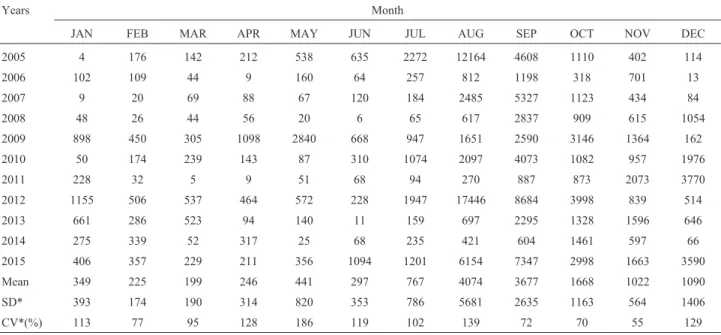
Table 1 shows the distribution of foci, the monthly averages, the standard deviations and the corresponding
co-efficients of variation for the series analyzed, from January to December, in the 2005-2015 period.
According to Table 1, the monthly averages in the pe-riod 2005-2015 presented considerable increase from July on, with a peak in August and September, reaching maxi-mum values (4074 and 3677 foci, respectively). The stan-dard deviations and hence the coefficients of variation present high values, indicating a large heterogeneity of data. This is understandable because, in the first semester, few fire foci occurred whereas in the second, the dry sea-son, a considerable increase was observed.
The period selected for the application of RLM and ARIMA forecasting techniques was, therefore, restricted to the months of July, August, September, October and No-vember of each year, known as the JASON (the first letter of each month) period that corresponds to the period with the highest concentration of foci events. For the analysis of time series, a cut was made in the number of foci detected only by the reference satellites NOAA-12 and NASA AQUA MT because they presented polar orbit, which gen-erates data that can be statistically analyzed for the same re-gions along the years with minimized errors and corrected atmospheric effects.
For performing the regression analysis, the base-10 logarithmic transformation was applied on the number of foci to stabilize the variance because of the great variability of these data, since the forecasts must be characterized by the accuracy of results, the simplicity of methods employed and the statistical reliability of the models used to generate predictions.
Table 1- Monthly statistics of the total number of foci, obtained from all satellites operating on the 4mm thermal band (NOAA- 12; NOAA-15; NOAA-16; NOAA-18; NOAA-19; NASA AQUA M-T; GOES-12; GOES-13 and MSG-2) for the total scanning of 24 hourly measurements per day from 2005 to 2015 in Corumbá (MS).
Years Month
JAN FEB MAR APR MAY JUN JUL AUG SEP OCT NOV DEC
2005 4 176 142 212 538 635 2272 12164 4608 1110 402 114
2006 102 109 44 9 160 64 257 812 1198 318 701 13
2007 9 20 69 88 67 120 184 2485 5327 1123 434 84
2008 48 26 44 56 20 6 65 617 2837 909 615 1054
2009 898 450 305 1098 2840 668 947 1651 2590 3146 1364 162
2010 50 174 239 143 87 310 1074 2097 4073 1082 957 1976
2011 228 32 5 9 51 68 94 270 887 873 2073 3770
2012 1155 506 537 464 572 228 1947 17446 8684 3998 839 514
2013 661 286 523 94 140 11 159 697 2295 1328 1596 646
2014 275 339 52 317 25 68 235 421 604 1461 597 66
2015 406 357 229 211 356 1094 1201 6154 7347 2998 1663 3590
Mean 349 225 199 246 441 297 767 4074 3677 1668 1022 1090
SD* 393 174 190 314 820 353 786 5681 2635 1163 564 1406
CV*(%) 113 77 95 128 186 119 102 139 72 70 55 129
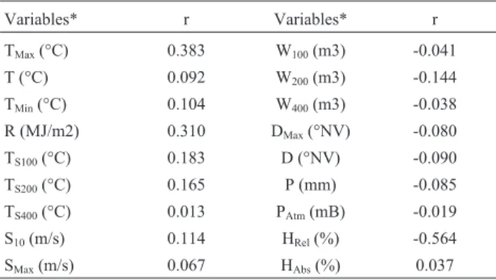
Table 2 shows the results of the linear correlation be-tween the variable related to the fire foci and its meteoro-logical predictor variables.
The negative values presented by correlations (r)
mean that the lower the value of the climate element, the higher the possibility of fire occurrences. However, if the value ofris positive, the higher the value of the parameter,
the lower the probability of occurring fire foci.
The meteorological variables that favor most the oc-currence of foci according to the correlation analysis for the application of the RLM and ARIMA methods are maxi-mum temperature, relative humidity and solar radiation, of which they presented more satisfactoryr.
The temperature affects the condition of the vegeta-tion, raising the internal temperature of the plant tissues, dissecting it and contributing to ignition and flammability. The solar radiation directly affects the duration of the pre-heating period prior to the onset of fire (Machadoet al.,
2014).
Relative humidity is the predictive factor that contrib-utes most to the burning process. Being a component in-versely proportional to the number of foci, it is directly related to the low rainfall, becoming a decisive factor for the occurrence of forest fires, since it affects the vegetation regarding humidity and the availability of oxygen in the plant, favoring the conditions that encourage the combus-tion process.
The soil temperature variable was not used in the analysis because it presents multicollinearity with the max-imum air temperature. The case is the same with the soil water count variable, already taken into account when ana-lyzing the relative humidity of the air that directly influ-ences this variable. The wind velocity variable was not considered either as it is directly related to the propagation of fire rather than to its onset.
The other predictive variables disregarded in the re-gression model explain the phenomenon in less than 2% be-cause they are indirect terms already associated with the predictive factors.
Table 3 shows a comparison between the data of Ta-ble 2 and those found by Torreset al.(2011) on a study of
fire occurrence in Juiz de Fora (MG).
The correlations of the most significant environmen-tal parameters were close to the meteorological variables analyzed, differing only as to the temperature variable, which is explained by the geographic and climatological differences of the two regions compared.
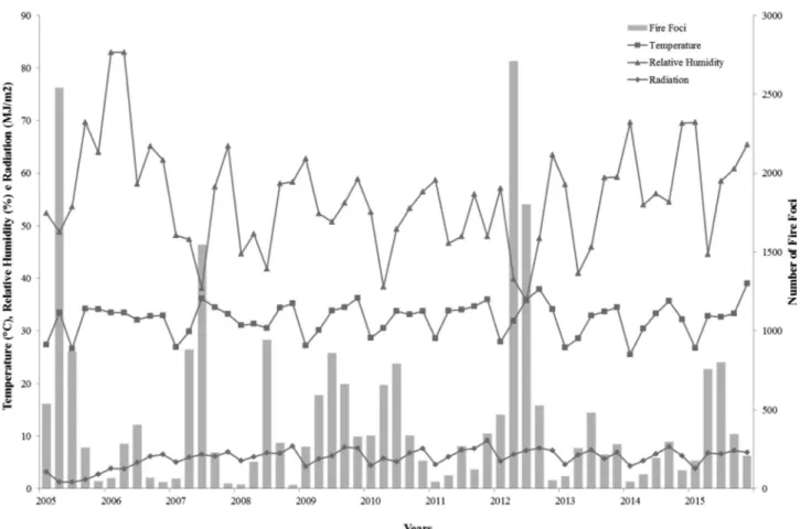
The monthly variability for the JASON period in the 2005-2015 time series of the number of foci, maximum temperature, relative humidity and solar radiation are shown in Fig. 1, where the profile of the associated burn-ings can be observed over time, associated with these envi-ronmental variables.
In general, the highest values of foci correspond to the lowest values of relative humidity, showing the inverse cor-relation between these two variables, as can be observed for the month of September of 2007 and 2012. The low relative humidity of the air directly influences the vegetation, mak-ing it drier, which facilitates the increase of combustible material and consequently the susceptibility to the combus-tion process. The peaks of foci occurred in August and Sep-tember of the dry season with an average value of 450 foci.
The mean maximum temperature was 32.3 °C and it can be observed that for the higher temperatures the num-ber of foci is higher, such as August 2005, Septemnum-ber 2007, August and September 2012 and November 2014. The tem-perature showed a significant correlation with the number of foci, but it must be associated with the factor of low rela-tive humidity so that it can be significant within the models, because if the temperature is high and so is the relative hu-midity of the air, a decrease in the number of foci can be ob-served, for instance in the months of August 2006 and October 2013.
Solar radiation presented maximum value of 9.2 MJ/m2, however a high rate does not mean that the
num-ber of foci will be the highest because its incidence is di-rectly affected by the presence of clouds. When low humidity and high temperature occur, the curves are pre-sented in phase, but when analyzed separately, there are
Table 2- Pearson’s correlation coefficient test (r) between the occur-rences of fire foci and the studied environmental variables in the period 2005-2015 in Corumbá (MS).
Variables* r Variables* r
TMax(°C) 0.383 W100(m3) -0.041
T (°C) 0.092 W200(m3) -0.144
TMin(°C) 0.104 W400(m3) -0.038
R (MJ/m2) 0.310 DMax(°NV) -0.080
TS100(°C) 0.183 D (°NV) -0.090
TS200(°C) 0.165 P (mm) -0.085
TS400(°C) 0.013 PAtm(mB) -0.019
S10(m/s) 0.114 HRel(%) -0.564
SMax(m/s) 0.067 HAbs(%) 0.037
*Were: Instant Air Temperature (T); Maximum Air Temperature (TMax); Minimum Air Temperature (TMin); Soil Temperature at 100, 200 and 400 mm (TS 100, 200 and 400); Rainfall P; Relative Humidity (HRel); Absolute Hu-midity (HAbs); Wind Speed at 10 meters (S10); Atmospheric Pressure (PAtm); Accumulated Solar Radiation (R); Soil Water Count at 100 mm, 200 mm and 400 mm (W100,200,400).
Table 3- Comparison of Pearsons correlation coefficient test (r) between the occurrence of fire foci in the Pantanal of Corumbá and in Juiz de Fora (MG) related to the same environmental variables.
Meteorological variable Correlations (r)
Corumbá (MS) Juiz de Fora (MG)
Solar radiation 0.310 0.357
Maximum air temperature 0.383 0.182
lags between the curves of foci and radiation. It can be ob-served that in September 2007 the curves are in phase and in November 2014 the radiation and temperature are high, however, because of the high relative air humidity the oc-currence of foci decreases.
The years 2005 and 2012 should be highlighted for they presented the highest rates of incidence of foci in the series. This is due to the accumulation of fuel material from the plants in the previous years (2004 and 2011, respec-tively) when high-level floods were reported in the county. The vegetation then turned weaker and propitious to burn-ing when submitted to the climatic conditions of the high temperatures and solar radiation and low relative air hu-midity in the following years, as can be observed in Fig. 1.
The years 2006, 2011 and 2014 presented a mean number of foci of 170 records, a lower rate resulting from the high relative humidity with the average over 60%.
The Multiple Linear Regression model of fire fore-cast in Corumbá (MS) is presented in Eq. (3), using the more significant predictor variables of the correlation ap-plied in relation to the number of foci. No multicollinearity was seen between variables, as the tolerance presented val-ues higher than 0.1 and the Variance Inflation Factor (VIF) values were less than 10, as expected.
log(N$)=1335 0032. - . R-0028. H+0050. T (3)
whereN$is the estimated value for the number of fire foci;R
is the accumulated solar radiation;His the relative
humid-ity; andTis the maximum daily temperature.
In Table 4 it is possible to observe the descriptive sta-tistics of the applied regression model, with log(N$)as a de-pendent variable, and the predictors given by variables Solar Radiation, Relative Humidity and Temperature.
The value obtained fromR2= 0.411 indicates that the fit degree of the predictive variables was 41%, with
Figure 1- Profile of the variability of the monthly averages of meteorological data (Temperature, Radiation and Relative Humidity) and comparison with the total number of foci for the JASON period from 2005 to 2015 in Corumbá-MS.
Table 4- Descriptive Statistical Analysis of the RLM.
R Square R Estimate standard error Statistics Durbin-Watson
Square R change F change F change
p < 0,0001, explaining the output variability , given the me-teorological predictors.
The MAPE was 33.9% among the actual values of the base-10 logarithm of the number of foci for the values esti-mated by Eq. (3), obtained for the same values of environ-mental variables of the time series analyzed. In applying Stein to the value ofR2it can be seen that the result was
close to the fit value of 0.410, which means that the model can be generalized for different samples and that the cross-validation of the model occurred.
The statistical analysis resulted in the change of F = 390.034, where new predictor variables inserted in the model by the configuration of IBM-SPSS in stepwise mode were satisfactory for the prediction of foci number, how-ever the hypothesis of independence of errors analyzed by the Durbin-Watson test was partially satisfactory, resulting in 0.917.
Given these analyses, it can be seen that the MLR technique is not the most suitable model for predicting the number of foci, since the model did not seem to be strictly linear. It has yet to be taken into account the possibility of inserting other variables that can contribute to an improved performance of this method, such as a variable associated with anthropic actions.
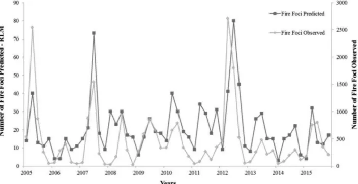
The results of the comparison of the observed and the MRL-predicted fire foci are represented in Fig. 2.
According to Fig. 2 it is possible to confirm that the graphs of the observed and the predicted data are in phase with peaks of coincidental maximum and minimum values and tonicities with the same characteristics along the whole
curve, in different scales because they have been applied in a parameterized way in the regression using base-10 loga-rithm.
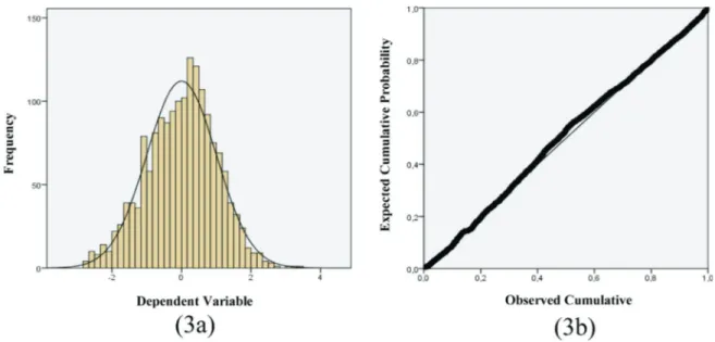
The residual analysis is plotted in Fig. 3 with the stan-dard distribution residual histogram graphs (Fig. 3a) and the standard regression distribution of the standardized re-siduals of observed and predicted cumulative probability (Fig. 3b).
Considering the analysis of residuals, it can be ob-served that the model can be used to make inferences be-yond the sample of data used, however it is not the most suitable model for the forecast of the foci because it is not a strictly linear characteristics model and Not to include anthropic action in its predictive variables, which justifies a residual error higher than 60%.
The model is able to explain the variance of the mete-orological variables for the prediction of foci as to how pro-pitious they are to occur. In order to improve the prediction of how many foci will occur it is necessary to insert vari-ables that specify the causes of occurrence of each focus (natural or anthropic).
Table 5 shows the result of the application of the Autoregressive Integrated Moving Averages technique – Box-Jenkins’s ARIMA – with four autoregressive terms and ten moving average terms.
It was not necessary to differentiate, that is,d= 0,
be-cause data were stationary. The number of autoregressive orders was p = 4, requiring four time periods of the series in the past to predict the current value. The value ofq= 10
specifies that the deviations of the mean values of the series
of each of the last ten time periods are considered when pre-dicting the current values of the series. The analysis of the Bayesian information criterion showed that the ARIMA
model (4, 0, 10) is the best predicting model associated with significance p < 0.005. In addition, it is observed that the model fit turns out to be 66.5%, with a mean absolute
per-Figure 4- Comparative graph of the number of predicted and observed foci by the ARIMA model for the JASON period of the historical series
2005-2015 of Corumbá-MS.
Figure 3- Residual graph of the MRL model. (3a) represents the histogram of the frequency-dependent variablevs.the standardized residuals regression. (3b) represents the standardized residual values of the expectedvs.observed probability.
Table 5- Descriptive Statistical Analysis of the ARIMA.
Model Statistics Ljung-Box Q(18)
Number predictors R2 RMSE MAPE MAE BIC normalized DF p-value
ARIMA (4, 0, 10) 3 0.665 0.484 31.597 0.381 1.398 11 0.001
centage error (MAPE) of 31.6%, considerably improving the overall performance of the ARIMA model when com-paring with the RLM model.
The comparative graph of observed and predicted foci values for the ARIMA forecasting technique is shown in Fig. 4.
From Fig. 4 it is possible to observe that the curves of the predicted and estimated values are in phase and present the coincidental conditions of tonicity and the peaks of maximum and minimum with the same delineation.
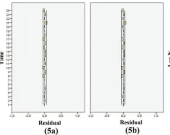
Figure 5 shows the graphs of the residual autocorre-lation function (Fig. 5a) and the partial residual autocor-relation function (Fig. 5b) for the ARIMA technique.
The analysis of residuals and the Durbin-Watson test (D= 1.97) showed that the error interdependence
hypothe-sis is satisfied and the overall ARIMA performance was 68.4% with p < 0.002. It is then able to forecast five steps ahead with the same accuracy, as shown in the five catego-ries represented in the graph of Fig. 5, not being necessary the forecast values of the meteorological variables for that same period.
The residual graph analysis revealed that the model is well fitted, since it presents values very close to zero. The estimators are not biased and the ARIMA model presented significantly better results to predict data output of the number of foci.
4. Conclusions
The meteorological factors analyzed establish an im-portant relation with the conditions of vegetation, and di-rectly affect the occurrence of fire points and forest fires, of which the solar radiation, relative air humidity and temper-ature are enhanced.
It was possible to determine the profile of fire points in the Pantanal biome associated with the meteorological
variables and it was observed that the months with the greatest water deficit (JASON period) presented the highest incidence of foci. It is vital to consider that the risk of fire is associated with how propitious the vegetation is under spe-cific meteorological conditions of beginning the combus-tion process. These estimates, however, do not consider the anthropic factors because of the lack of databases available for this quantification.
Multivariate data analysis techniques were applied by MLR and ARIMA models, where the former explained 41% of variance of the number of foci, thus showing to be a non-efficient technique for prediction.
The modeling of time series using the ARIMA tech-nique (4, 0, 10) presented more satisfactory results, making it possible to explain the variance of the number of foci in 66.5%, which proves to be the most adequate model for forecasting. In order to improve the performance of this technique, the anthropic variable should be inserted, which is a decisive factor for fires to occur, but it is necessary to build such a database so that the performance of new fore-cast models can be improved.
References
ARTAXO, P.; OLIVEIRA, P.H.; LARA, L.L.; PAULIQUEVIS, T.M.; RIZZO, L.V.; JUNIOR, C.P. Efeitos climáticos de partículas de aerossóis biogênicos e emitidos em queimadas na Amazônia.Revista Brasileira de Meteorologia, v. 21, n. 3a, p. 168-189, 2006.
BRASIL. RADAMBRASIL, Ministério das Minas e Energia.
Folha SE. 21. Corumbá e Folha SE. 20. Geologia, Pedo-logia, GeomorfoPedo-logia, Vegetação e Uso e Ocupação da Terra. Rio de Janeiro, 1982, 448 p.
DEPPE, F.; PAULA, E.V.; MENEGHETTE, C.R.; VOSGERAU, J. Comparação de índice de risco de incêndio florestal com focos de calor no Estado do Paraná.Floresta, v. 34, n. 2, p. 119-126, 2004.
ESPINOSA, M.M.; PRADO, S.M.; GHELLERE, M. Uso do modelo SARIMA na previsão do número de focos de calor para os meses de junho a outubro no Estado de Mato Grosso.
Ciência e Natura, v. 32, n. 2, p. 7-21, 2010.
FIEDLER, N.C.; MERLO, D.A.; MEDEIROS, M.B. Ocorrência de incêndios florestais no Parque Nacional da Chapada dos Veadeiros, Goiás. Ciência Florestal, v. 16, p. 153-161, 2006.
GRANEMANN, D.C.; CARNEIRO, G.L. Monitoramento de fo-cos de incêndio e áreas queimadas com utilização de ima-gens de sensoriamento remoto.Revista de Engenharia e Tecnologia, v.1, n. 1, p. 55-62, 2009.
HAIR Jr., J.; ANDERSON, R.; TATHAM, R.; BLACK, W.
Análise multivariada de dados.5ª Ed. Porto Alegre: Book-man, 2005, 596 p.
IBGE.Instituto Brasileiro de Geografia e Estatística. Cidades Mato Grosso do Sul – Corumbá MS. Disponível em: http://www.cidades.ibge.gov.br/xtras/perfil.php?lang=&co dmun = 500320&search=mato-grosso-do-sul corumba infograficos:-informacoes-completas. Acesso em: 08 fev. 2016.
IMASUL.Instituto de Meio Ambiente de Mato Grosso do Sul.
Disponível em: http://www.imasul.ms.gov.br. Acesso em: 21 jan. 2016.
INMET.Instituto Nacional de Meteorologia.Banco de Dados Meteorológicos para Ensino e Pesquisa. Disponível em:
http://www.inmet.gov.br/portal/in-dex.php?r=bdmep/bdmep. Acesso em: 08 fev. 2016. INPE. Instituto Nacional de Pesquisas Espaciais. Portal do
Monitoramento de Queimadas e Incêndios. Disponível em: http://www.inpe.br/queimadas. Acesso em: 08 fev. 2016. LEVINE, D.M.; STEPHAN, D.; KREHBIEL, T.C.;
BEREN-SON, M.L. Estatística –Teoria e aplicações usando o Microsoft Excel. 3ª ed. Rio de Janeiro/RJ: Ed. LTC, 2005, 819 p.
LONGO, K.M.; FREITAS, S.R.; SILVA DIAS, M.A.F.; SILVA DIAS, P.L. Emissões de queimadas em ecossistemas da América do Sul.Estudos Avançados, v. 19, n. 53, p. 167-185, 2005.
MACHADO, N.G.; SILVA, F.C.P.; BIUDES, M.S. Efeitos das condições meteorológicas sobre o risco de incêndio e o número de queimadas urbanas e focos de calor em Cuia-bá-MT, Brasil.Ciência e Natura, v. 36, n. 3, p. 459-469, 2014.
MAGI, B.I.; RABIN, S.; SHEVLIAKOVA, E.; PACALA, S. Sep-arating agricultural and non-agricultural fire seasonality at regional scales.Biogeociences, v. 9, p. 3000-3012, 2012.
MORETTIN, P.A.; TOLOI, C.M.C.Análise de séries
tempo-rais. 2ª ed. São Paulo/SP: Ed. Edgard Blüncher, 2006, 531 p. NOGUEIRA, J.S.; MUSIS, C.R.; SALLO, F.S.; PRADO, M.J.; PALÁCIOS, R.S. Análise da profundidade ótica de aeros-sóis e coeficiente de angstrom no cerrado Mato-Grossense.
Revista Brasileira de Climatologia, v. 14, n. 1, p. 173-182, 2014.
NOGUEIRA, J.S.; SANTOS, A.C.A. Análise do material parti-culado no Pantanal Mato-Grossense.Revista Brasileira de Meteorologia, v. 30, n. 3, p. 254-264, 2015.
PEREIRA, A.A.; PEREIRA, J.A.A.; MORELLI, F.; BARROS, D.A.; ACERBI JR., F.W.; SCOLFORO, J.R.S. Validação de focos de calor utilizados no monitoramento orbital de queimadas por meio de imagens TM.Cerne, v. 18, p. 335-343, 2012.
SILVA, R.A. Incêndio Florestal. In: TOCCHETTO, D.Perícia Ambiental Criminal.1 ed. Campinas: Millennium, 2014. p. 351-406.
SOARES, R.V.; BATISTA, A.C.; NUNES, J.R.S.Incêndios flo-restais no Brasil: O estado da arte.1 ed. Curitiba: Pro-dução Independente, 2009. 246 p.
SOBRINHO, T.A.; OLIVEIRA, P.T.S.; RODRIGUES, D.B.B.; AYRES, F.M. Delimitação Automática de Bacias Hidro-gráficas utilizando SRTM.Revista Brasileira de Engen-haria Agrícola e Ambiental, v. 30, n. 1, p. 46-57, 2010. SORIANO, B.M.A.; PELLEGRIN, L.A. Monitoramento do
nú-mero de focos de calor e variáveis meteorológicas obser-vados em 2007 no Pantanal. Comunicado Técnico, 64. Corumbá: Embrapa Pantanal, 2007. 3 p.
TORRES, F.T.P.; RIBEIRO, G.A.; MARTINS, S.V.; LIMA, G.S. Correlações entre os elementos meteorológicos e as ocorrên-cias de incêndios florestais na área urbana de Juiz de Fora, MG.Revista Árvore, v. 35, n. 1, p. 143-150, 2011. VIEIRA, H.J.; BACK, A.J.; LOPES F.; MORAIS, H. Estimativa
das temperaturas médias diárias, diurnas e noturnas a partir das temperaturas horárias. Revista Brasileira de Meteo-rologia, v. 27, n. 3, p. 329-336, 2012.