Neural Network Based Model Refinement

Neural Network Based Model Refinement

Adrian VIŞOIU

Academy of Economic Studies Bucharest Economy Informatics Department

In this paper, model bases and model generators are presented in the context of model refinement. This article proposes a neural network based model refinement technique for software metrics estimation. Neural networks are introduced as instruments of model refinement. A refinement technique is proposed for ranking and selecting input variables. A case study shows the practice of model refinement using neural networks.

Keywords: model refinement, neural network, software metrics, model generators.

Model bases and model generators Model bases are software structures for managing models, generating models, mana-ging datasets, manamana-ging modeling problem definitions as shown in [IVAN05].

Model generators are software instruments for obtaining models from a certain model class given the list of variables, the model structure, existence restrictions and datasets. They also have an important place in the refinement process flow.

Model classes group models with the same structure, e.g. linear models, linear models with lagged variables, nonlinear models. For each class a model generator is developed as a software module. Each dataset contains data series for the recorded variables. The dependent variable is specified and the generator builds analytical expressions using influence factors, coefficients, simple ope-rators and functions. For each model structure, coefficients are estimated and a performance indicator is computed. The resulting model list is ordered by the performance indicator. The analyst chooses between the best models an appropriate form that later will be used in estimating the studied characteristic.

Linear model generators take as input a dataset containing a number of independent variables and a dependent variable and produce linear models by combining influence factors.

The practice conducted to the elaboration of linear models because: the studied phenomena aim a linear dependence, the parameter estimation methods are customary

for this type of models, the results interpretation is lightened if the linearity hypotheses are taken into account. The linear generators take as input: the list of independent variables, the dependent variable, the dataset, restrictions about the dimension and the complexity of the model, performance criterion for all generated models. The output consists of: the list of generated models ordered by the perfor-mance criterion.

In [VISO06] nonlinear generators are described. Standard nonlinear model generators use predefined analytical forms for generating models. General nonlinear model generators build automatically analytical expressions containing influence factors. The parameters for this process are: the operand set, the coefficient set, the operator set, the maximum complexity of the generated expression. The nonlinear model generator is suitable for modeling as the phenomena do not always follow linear laws. The linear models generators with delayed arguments allow the elaboration of constructions which permit the modeling of the multiple stimulation effects which are found on short term in influences from all the sets. The phenomenon evolution shows that the factors differently influence the dependent variable. More, the variation at a moment t of a factor spread them with a delay abroad the evolution of the dependent variable. The delayed arguments model generator takes the same inputs, as the linear generator, but it also does not only combinations of variables, but also

combinations of delays for the variables included in a certain model. As a new parameter for this algorithm, the maximum allowed delay is taken.

Model generators are important instruments for the different refinement methods, but also generally for model design.

Artificial neural networks are nonlinear models used as modern instruments for:

− regression analysis

− classification

− data processing.

In this paper, neural network’s capacity to estimate evolution of nonlinear phenomena is used as instrument for model refinement and variable list refinement.

2. Refinement using neural networks In [IVAN05] the problem of building models is presented in detail and in [VISO05] the problem of software quality estimation model refinement is treated in detail.

When used for regression analysis, neural networks are considered nonlinear models used estimate the level of a dependent variable given the values for the independent variables. The performance of neural networks is, most of the time, better than classic models. Its capacity is given by the internal complexity. In the following, a feed forward multilayered network with backpropagation learning algorithm is taken into account.

The network structure consists of connected neuron layers. When estimating levels for dependent variables the input layer takes the input values. It has as many units as the number of inputs.

The hidden layer is placed between the input and the output layers. Each unit in the input layer is connected to each unit in the hidden layer. Further, each unit in the hidden layer is connected to each unit in the output layer. Connections transfer the output from a source neuron as input to a destination neuron, applying a weight.

The output layer consists of neurons delivering the output of the network.

The inputs are all normalized in the (0, 1) interval. The network also outputs a value in (0, 1) interval. The value has to be de-normalized before using the result, by applying an inverse transformation. The values for the considered inputs are real positive numbers, bounded by zero and a maximum value for each type of input.

Consider a network NNET consisting of three layers, an input layer with n units, a hidden layer with h hidden units and an output layer consisting of one unit. The activation function is the Sigmoid function denoted by

f. Let wij denote the weight of the ith input in

the activation of jth unit in the hidden layer. Let ujk denote the weight of output of the jth

hidden in the activation of kth output unit. The inputs are denoted by I1, I2, …, In.

The activation for the jth hidden unit is given by

Aj = w1j*I1+w2j*I2+...+wnj*In-Tj, j=1,h

and it has:

− 2n operators

− 2n+1 operands.

The complexity in Halstead sense of the activation model for the jth unit is:

C(Aj) = 2nlog2 2n +(2n+1)log2(2n+1)

The output for the jth hidden unit is given by

Oj = f(Aj)=1/(1+e-Aj)

and it has:

− (2n+3) operators

− (2n+4) operands.

The complexity in Halstead sense for the output model for the jth unit is:

C(Oj) =

(2n+3)log2(2n+3)+(2n+4)log2(2n+4)

The activation of the output unit r is given by

Ar = u1r*O1+u2r*O2+...+ uhr*Oh-Tr

and there are:

− 2h + h*(2n+3)= 2nh+5h operators

− (h+1)+h(2n+4)= 2nh+5h+1 operands The output of the network is:

Or = f(Ar)=1/(1+e-Ar)

and it has:

− 2nh+5h+3 operators

− 2nh+5h+4 operands

In general, the model complexity for an output of the network is

If the network has a number of R output units, then for the output values there are R

models with C(Or) complexity.

When using neural networks, the number of output units is established and it is a fixed number because it is usually known what is to be estimated. The number of hidden units becomes fixed after an empirical study by testing different values, or by an empirical formula. The inputs are chosen among the variables associated to the factors, the analyst believes they influence the studied phenomenon. In order to see the importance of inputs in the overall complexity of the network, table 1 is built,

Table no 1. Evolution of an output unit model complexity for a network with n inputs, where the number of hidden units

is fixed, h=10 Inputs

n

Operators 2n+5h+3

Operands 2n+5h+4

Complexity C(Or)

1 73 74 911,36 2 93 94 1224,27 3 113 114 1549,63 4 133 134 1885,21 5 153 154 2229,47 6 173 174 2581,26 7 193 194 2939,73 8 213 214 3304,17 9 233 234 3674,02 10 253 254 4048,82 11 273 274 4428,18 12 293 294 4811,77 13 313 314 5199,29 14 333 334 5590,49 15 353 354 5985,16 16 373 374 6383,09 17 393 394 6784,11 18 413 414 7188,07 19 433 434 7594,82 20 453 454 8004,24 It is observed that after establishing the outputs and hidden layer size, further model refinement is necessary through reducing the number of inputs.

The inputs are all normalized to (0, 1). In the activation of jth hidden unit Aj, each input has

its own weight which shows the degree of influence for that activation

Due to the fact that input variables influences can be established and easily understood only at input-to-hidden level, the after training weights at input-to-hidden level are studied. The input values for the independent variables are normalized in the (0; 1) interval. This way, the weights become comparable. If a weight |wpj|>|wqj| the pth

variable from the input layer has more significance in the activation of j hidden unit than qth variable.

The technique for ranking the input variables according to their influence in a model aims decreasing the number of variables.

When building models, a number of factors are considered to influence the studied phenomenon and variables are associated to them in the model structure. These factors differ from their importance and some are more important than others. To achieve model refinement, the less important factors have to be eliminated. When dealing with nonlinear models it is difficult to assess each factor’s importance. The proposed technique uses neural networks as complex nonlinear models to assess the importance of each factor. Figure 1 shows a flow for model refinement using neural networks, and the place of this process in the refinement flow. Figure 1 shows that the model M is to be refined. The model M is from a certain model class, CM. The analytical expression for the model consists of a set of operators and a set of operands. The operands are further separated into a set of coefficients and a set of variables, denoted by V. The variables in V

M’ which is the refined model.

When using only neural networks for estimation, only the independent variable list and the dependent variable are needed. An initial network INET is built, having NI=card

(V) inputs. Through refinement, the input list is reduced to the V’ set, and further a second network RNET with NR=card(V’) inputs is built, where NR<NI, representing the refined network.

Model M of class CM

Operators

Variables V

Coefficients

Neural Network Refinement

Variables

Model generation

Model M’ of class CM Neural Network

estimation

Model processing Fig.1. Model refinement flow using neural networks

Looking at the considered network architecture, it is observed that each input is connected to each hidden node. In the activation Aj of the jth hidden node, each

input has a weight attached to it showing the importance of that input for the activation. All the inputs are normalized in (0; 1) interval, and thus the weights of connections to that unit are comparable from absolute value point of view.

If |wfj|>|wgj|, for the activation of jth hidden

unit being a linear model, the input If,

associated to the f factor, has a greater influence than the input Ig.

By summing up the absolute values of weights from If to each hidden unit, an

indicator is obtained showing the total absolute influence of input f, TAIf, given by:

TAIf =

∑

=

h

j 1

|wfj|

where h is the number of hidden units. An initial ordering of influence factors can be done by this indicator. The analyst can choose the first k variables to be later used in

model building.

Further, in the activation of jth hidden unit each input comes with its own weight. It is needed to compute the relative weight of If in

the sum of weights of synapses to the jth unit as:

w’fj =

∑

=

n

i

wij wfj

1

| |

| |

This relative weight is used in computing the total relative influence of If in the hidden

layer, as:

TRIf=

∑

=

h

j 1

w’fj

This indicator takes into account the influence of If paying attention to the

magnitude of the influence reported to other factors also. The independent variables can be ordered by this indicator and the analyst can choose among them, reducing the list of variables.

as:

TTRI =

∑

=

n

i 1

TRIi, where n is the number of

inputs.

Each TRI value is then divided by this sum, obtaining the normalized total relative influence as:

NTRIf = TRIf / TTRI, f=1,n.

This way the it is easier to choose the which variables corresponding to NTRI values are kept during the refinement as:

∑

=

n

i 1

NTRIi = 1.

The first N variables in the ordered list are kept with the restriction:

∑

=

N

i 1

NTRIi< t, t∈.(0,1), recommended value

used in this paper is t=0,85.

This aids the desicion of what variables to be removed because there is an instrument. As seen, the influence is assessed only at input-to-hidden level. That is because further than the first hidden layer, outputs contain already influences from all the inputs and

cannot be separated.

It is observed that the refinement process has an iterative character of the and the flow is finite with respect to a performance criterion. 3. Case study

For a group of 35 specialists involved in developing software modules in data structures field, implementing sparse matrix operations, data is collected regarding the number of hours necessary for module development, the number of errors encountered during code writing, the working experience in months in the field of software development, data about their performance as students, and metrics of the source code for each module. The specialists build up an homogenous sample based on selection criteria: age, experience and training.

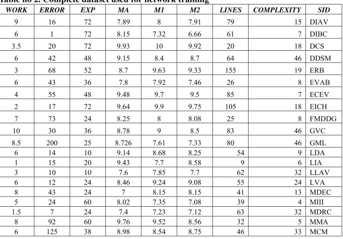
The dataset resulted from the activity analysis for the 35 specialists is presented in table 2. Data collection has been done automatically using software packages software metrics oriented.

Table no 2. Complete dataset used for network training

WORK ERROR EXP MA M1 M2 LINES COMPLEXITY SID

9 16 72 7.89 8 7.91 79 15 DIAV

6 1 72 8.15 7.32 6.66 61 7 DIBC

3.5 20 72 9.93 10 9.92 20 18 DCS

6 42 48 9.15 8.4 8.7 64 46 DDSM

3 68 52 8.7 9.63 9.33 155 19 ERB

6 43 36 7.8 7.92 7.46 26 8 EVAB

4 55 48 9.48 9.7 9.5 85 7 ECEV

2 17 72 9.64 9.9 9.75 105 18 EICH

7 73 24 8.25 8 8.08 25 8 FMDDG

10 30 36 8.78 9 8.5 83 46 GVC

8.5 200 25 8.726 7.61 7.33 80 46 GML

6 14 10 9.14 8.68 8.25 54 9 LDA

1 15 20 9.43 7.7 8.58 9 6 LIA

3 10 10 7.6 7.85 7.7 62 32 LLAV

6 12 24 8.46 9.24 9.08 55 24 LVA

8 43 24 7 8.15 8.15 41 13 MDEC

5 24 60 8.02 7.35 7.08 39 4 MIII

1.5 7 24 7.4 7.23 7.12 63 32 MDRC

8 92 60 9.76 9.52 8.56 32 5 MMA

3 17 6 8.71 8.66 9.33 72 32 NGGF

5 7 72 9.5 9.65 9.75 64 10 NOA

8 14 60 7.98 7.53 7.33 94 9 NIIAA

2 13 120 9.19 7.33 7.72 48 7 NCE

4 12 86 8.2 8.14 7.53 58 11 NGAD

2 7 72 9.43 8.53 9.25 26 11 NCAC

4 32 24 6.76 7.49 7.69 42 8 OIIA

4 10 72 9.84 9.56 9.18 55 13 ONF

3 11 86 8.89 7.23 7.16 70 11 OIM

4 23 26 8.32 9.32 8.91 87 12 OIC

3 4 36 9.53 9.5 9.75 14 6 PVRI

8 30 72 8.74 9.04 9.08 77 9 PIVC

3 7 10 8.83 8.2 7.66 24 9 PAIV

3 30 48 7.8 7.9 7.6 88 9 PGC

5 14 84 8.66 8.09 9.24 118 12 JIAC

The software collection used for research development and partial results can be found at http://www.refinement.ase.ro.

The variables displayed in columns are described as follows:

WORK – is the dependent variable representing the amount of time, in hours, necessary for developing a software module;

ERROR – the number of errors encountered during development;

EXP – the experience in months of the developer;

MA – the admission mean for the specialist in the higher education institution

M1 - the mean after the first year of study; it is interpreted as the level of basic knowledge necessary in the field of computer programming;

M2 – the mean after the second year of study; it is interpreted as the level of specialized knowledge in the field of computer programming;

LINES – the number of source lines in the developed module

COMPLEXITY – the cyclomatic complexity of the developed module

SID – an identifier for each specialist; it is not used as input but it is used for information retrieval.

A model is needed for estimating the WORK

variable, as dependent variable, using the other variables as independent variables. In order to refine the model, independent variables are ranked according to the magnitude of their influence in estimating the network output.

The network has seven inputs for the independent variables values, one output for the estimated variable and a hidden layer consisting of 3 units, denoted N1, N2, and N3.

The activation function is sigmoid and the learning algorithm uses backpropagation. When learning the network training continues until either an error threshold or a maximum iteration is reached. After the training is complete, the input-to-hidden weights are displayed in table 3.

Table no.3 Input-to-hidden weights after network training

N1 N2 N3

ERROR -0.3450461 -10.05542 8.041933 EXP -1.499351 8.842965 -3.005034 MA -7.080837 -0.2618634 -1.689898

M1 10.5699 -4.063118 10.30558

In table 3 at the intersection between a line i

and a column j, the weight wij shows the

influence of the ith input in the activation of the jth neuron. As the weights can have both positive and negative values the absolute values become important as they show the

magnitude of the influence. By summing up the influence from each input i the TAIi total

absolute influence of that input is obtained. Ranking the list of variables by this indicator, an initial ordering is obtained as shown in table 4.

Table no. 4. Absolute values for weights

N1 N2 N3 Sum of weights Rank ERROR 0.345046 10.055420 8.041933 18.442399 3

EXP 1.499351 8.842965 3.005034 13.347350 5

MA 7.080837 0.261863 1.689898 9.032598 7

M1 10.569900 4.063118 10.305580 24.938598 2

M2 0.004751 2.305199 8.620939 10.930889 6

LINES 3.306778 16.349740 11.929560 31.586078 1 COMPLEXITY 6.289078 4.750813 3.685927 14.725818 4 As seen in table 4, the ranking shows that the

ordering of variables associated to influence factors is: LINES, M1, ERROR, COMPLEXITY, EXP, M2, and MA.

To take into account the relative influence, each weight in column j is divided by the sum of weights in that column, the resulting relative weights being shown in table 5. Table no 5 Relative influences from input units to hidden units

N1 N2 N3

ERROR 0.011859 0.215647 0.170096 EXP 0.051532 0.189645 0.063560 MA 0.243363 0.005616 0.035743 M1 0.363280 0.087137 0.217974 M2 0.000163 0.049437 0.182342 LINES 0.113652 0.350634 0.252323 COMPLEXITY 0.216151 0.101885 0.077961

TOTAL 1 1 1

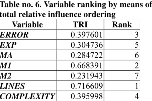
Summing up the value for each line i, the total relative influence TRIi of ith input is

obtained. Input variables can be ranked by this criterion as shown in table 6.

Table no. 6. Variable ranking by means of total relative influence ordering

Variable TRI Rank

ERROR 0.397601 3

EXP 0.304736 5

MA 0.284722 6

M1 0.668391 2

M2 0.231943 7

LINES 0.716609 1

COMPLEXITY 0.395998 4

As seen in table 6, the order of variables according to factor importance in the studied phenomenon is: LINES, M1, ERROR, COMPLEXITY, EXP, MA, and M2. As the neural network is assimilated to a nonlinear model, a conclusion can be drawn that there exists a nonlinear model to estimate WORK

variable built on those independent variables. Ordering variables according to the resulting rank can lead to the decision of removing less important variables, obtaining:

-a decreased complexity of the network leading to faster training and faster forward propagation

-better understanding of influence factors ranking for the studied phenomenon

networks can be used as input for other processes such as model generation.

Further, the variable list is reordered by their relative influences. The normalized total

relative influence values, NTRI are computed and also the cumulative sum, shown in table 7.

Table no. 7. Variable list ordered by TRI

Variable TRI NTRI

Cumulative sum LINES 0.716609 0.238870 0.238869531

M1 0.668391 0.222797 0.461667

ERROR 0.397601 0.132534 0.594200 COMPLEXITY 0.395998 0.131999 0.726200

EXP 0.304736 0.101579 0.827778

MA 0.284722 0.094907 0.922686

M2 0.231943 0.077314 1.000000

TOTAL 3 1 -

The chosen variables are those with the cumulative sum less than 0,85: LINES, M1, ERROR, COMPLEXITY, EXP.

Taking decisions based on the neural networks is desired, but they lack in transparency. It is difficult to argument a decision to another person based on a neural network because even if the inputs and outputs are very clear for the majority of the specialists, the transformations suffered by the input data is hard to both to interpret and explain. A regression model in the classical acceptance, seen as an analytic expression is far more explicit. It may not have the same performance as a neural network but it is transparent and can be more easily interpreted and explained.

Refining the neural network reduces the number of inputs necessary for estimation. If the network is not further used for estimation, the remained variables are used as input for model generation, using a model generator from a certain model class. If also a neural network is used for estimation, a second network is built having as inputs, the variables obtained from refinement, training is done and then validation is performed by comparing the initial network error with the second network error to see if the second network performance is acceptable.

4. Conclusions

The proposed method is used directly for the

refinement of any software quality model in which a list with many variables has been defined, collecting of all data is done automatically and the precision of the estimates is kept in an interval when a sublist of variables is used.

To trust neural network based refinement methods, the analysts which build software metrics will use classical refinement methods simultaneously. Results are compared and it is observed that neural network based refinements are most of the time more precise. The analyst will use just neural networks only after validation.

Neural network based refinement is an iterative process, the performance criterion being given by the errors the refined model generates as presented in [IVAN08].

Neural network based refinement is a new research area and the study of refined models must be further developed. The neural network based refinement technologies will be further developed including other types of neural networks.

If the current research used homogenous sets of C++ programs, research must be extended for heterogeneous sets of programs as problem typology and programming languages.

same way the modelbase is developed, software must be designed for refined model management, for user problem definition and for the study of real life behavior of refinement models.

Bibliography

[BODE02] Constanţa Bodea - Inteligenta artificiala: calcul neuronal, Editura ASE, Bucureşti 2002, ISBN 973594085X

[HILL06] Thomas HILL, Pavel LEWICHI -

Statistics: Methods and Applications: a Comprehensive Reference for Science, Industry and Data Mining, StatSoft Inc.2006, ISBN 1884233597

[IVAN05] Ion IVAN, Adrian VIŞOIU - Baza de modele economice, Editura ASE, Bucureşti, 2005

[IVAN08] Ion IVAN, Adrian VIŞOIU –

Tehnici de rafinare a metricilor software. Teorie şi practică, Editura ASE, Bucureşti 2008, to appear soon

[IVAN99] IVAN, Mihai POPESCU - Metrici software, Editura Inforec, Bucureşti, 1999

[JUDD] J. Stephen JUDD - Neural Network Design and the Complexity of Learning, MIT Press 1990, ISBN 0262100452

[MATI05] Randall MATIGNON, Neural Network Modeling Using SAS Enterprise

Miner, AuthorHouse 2005, ISBN

1418423416

[VISO05] Ion IVAN, Adrian VIŞOIU

-Rafinarea metricilor software, Economistul, supliment Economie teoretică si aplicativă, 29 august 2005, nr.1947(2973)

[VISO06] Adrian VIŞOIU, Gabriel GARAIS: Nonlinear model structure generator for software metrics estimation, The 37th International Scientific Symposium of METRA, Bucharest, May, 26th - 27th, 2006, Ministry of National Defence, published on CD