Numerical study of ground vortex formation

Universidade da Beira Interior

MANETA M. Alexandre

Numerical Study of Ground Vortex Formation

University of Beira Interior

Aerospace Sciences Department of University of Beira Interior

MSc Project

Academic Year 2008-2009

MANETA M. Alexandre

Numerical Study of Ground Vortex Formation

Supervisor: J. M. M. Barata June 2009

To my Parents and Sisters

Life to be appreciated, tasted and really lived, must be shared

with the ones we care, protect and enjoy.

Abstract

It is well known that under certain conditions, a tornado-like vortex is formed between an air inlet and a nearby solid wall. When a gas-turbine engine is operated / manoeuvred near a ground plane at static or near-static conditions, a strong vortex is often observed to form between the ground and the inlet. This so called inlet vortex (or ground vortex) can cause severe operational difficulties.

With CFD tools, the ground vortex phenomenon has been simulated on a 1/1th _scale

model. Calculations have been performed under cross-wind ground vortice mode of formation. The effect of the height of the intake to the ground and the effect of the cross-flow velocity have been studied in term of velocities and turbulent kinetic energy, after which the study of the appearance and location of the vortice have been made. The cross-flow test showed the formation of one vortice at an upstream location. The study of the effect of cross-flow velocity and the effect of the height of the intake showed that are fulcral parameters for the appearance and strength of the vortice.

Acknowledgments

I would like to express my thanks and appreciations to my supervisor, Professor Jorge M. M. Barata, for his guidance, support and opportunity to be part of the AeroG - Aeronautics and Astronautics Research Center while student in UBI – University of Beira Interior. I wish to thank Professor André R. R. Silva for the help he gave me during the thesis. I would like to thank the support of the Aerospace Sciences Department of University of Beira Interior for helping all these years the students with their problems.

I also would like to thank my best friends, Nuno Bernardo, Paulo Correia and Samuel Ribeiro, for making my stay in Covilhã bearable and really enjoyable.

I also would like to thank my parents for sponsoring all these years as student and for giving me the inspiration and initiative to pursue my dreams. Finally I would like to thank my sisters for always giving me reasons to smile while facing problems.

Index

1.3.2 Core vortex characteristics ... 19

1.3.3 Formation of inlet ground vortices ... 20

1.3.3.1 Criteria for intake vortex formation ... 20

1.3.3.2 Modes of formation ... 21

1.3.3.2.1 Mode one: Intake with no-wind ... 22

1.3.3.2.2 Mode two: Intake in head-wind ... 23

1.3.3.2.3 Mode three: Intake in cross-wind with irrotational flow ... 25

1.3.3.2.4 Mode four: Intake in cross-wind with ambient vorticity ... 28

Intake in tail wind ... 28

2 Mathematical Method ... 29

2.1 Introduction ... 29

2.2 Governing Differential Equations ... 29

2.3 Finite-Difference Equations ... 30

2.4 Solution Procedure ... 32

2.6 Grid independence ... 33

2.7 Summary ... 34

3 Results ... 35

3.1 Introduction ... 35

3.2 Geometry Model ... 35

3.3 Effect of the Height of the Intake ... 36

3.4 Effect of the Cross-Flow Velocity,   ... 37

3.5 Results from the cross-wind test case, ⁄ 9.9 ... 38

5 Conclusions ... 45

List of Tables

Table 1: Turbulence model constants. ... 28

Table 2:Test-Case conditions ... 35

List of Figures

Figure 2: Streamtube contraction ratio, / . ... 15

Figure 3: Intake flowfield in static configuration (a) and when flow separation appears (b). ... 16

Figure 4: Vortex line and vortex tube representations. ... 18

Figure 5: Consequences of vortex stretchin. ... 18

Figure 6: Idealization of the tangential velocity inside a tip vortex. ... 19

Figure 7: Inlet capture surface above the ground. ... 20

Figure 8: Data showing the boundary between the vortex forming and non-vortex forming flow regimes. Where Vi/Vo = / .. ... 21

Figure 9: Sense of rotation of the counter-rotating vortices with no wind. ... 22

Figure 10: Vortex filament in no-wind mode. ... 23

Figure 11: of rotation of the inlet vortices for a) low, b) medium and c) high velocity ratios. ... 23

Figure 14: Reason explaining the sense of rotation of the counter rotating vortices at low velocity ratio. ... 25

Figure 12: Vortex filaments in head-wind. ... 24

Figure 13: Vortex filaments in head-wind. ... 24

Figure 15: Reason explaining the sense of rotation of the counter rotating vortices at high velocity ratio. ... 25

Figure 17: Separation line around the inlet seen from the top view. ... 26

Figure 18: Flow aspects for low (<10 say) (a) ; and high (>20) (b) velocity ratios for an inlet in 90° cross-wind with an irrotational upstream flow. ... 27

Figure 19: Vortex formation in cross-wind with a upstream vertical vorticity. ... 28

Figure 20: Nodal configuration for the west face of a control volume. ... 31

Figure 21: Nodal configuration for a control volume. ... 32

Figure 22: Domain of the solution a). Representation of the intake with centered referential b). ... 33

Figure 23: Dimensionless Vertical profile, at X/D=0.53, of the horizontal velocity component, W, at a Z=0.1. ... 34

Figure 24: Configuration used in the Test-Case simulation. ... 35

Figure 25 Flow patterns for / equal to 0.97 (a), 1.02 (b), and 1.20 (c) in the plane facing the intake on a Y plane Y=Ymax. ... 36

Figure 26: Flow patterns for /  equal to 9.9 (a), 9.4 (b), and 8.7 (c) at X=2.75. ... 37

Figure 27 : Flow pattern and isolines of W for / 0.97 and / 9.9. ... 39

Figure 28 : Isolines of U,V and k in the vertical plane of symmetry at

X=0 ( / =0.97, 

and  /

=9.9)

Figure 29: Isolines of U,V, W and k in the vertical plane which contains the the engine axis (at Z=Zmax/2), and perpendicular to the crossflow ( / =0.97, and / =9.9). . 41

Figure 30 : Isolines of pressure in (a) ground plane, X=h, (b) plane parallel to the axis intake and the ground, X=h/2, and (c) plane containing the axis of the intake, X=0, ( / =0.97, and / =9.9). ... 42

Figure 31 : 3D particle visualization showing the formation and location of a vortice ( / =0.97, and / =9.9). ... 44 

Nomenclature

Variable Definition

Units

Area at intake throat 2

Far field area 2

Highlight diameter Inner diameter of intake

h Height of the engine axis above ground

k Turbulent kinetic energy 2_/ 2

Intake stream tube length m

Mass flow /

Throat Velocity /

∞    Free stream velocity /

Tangential velocity Greek Symbols Γ Vortex circulation / Vorticity / Density / Kinematic Viscosity / Dynamic Viscosity / .

Turbulent kinematic viscosity

Dependent Variable

1 Introduction

1.1 Introduction

Nowadays civil airplanes engines are designed to be quieter and more efficient. So to achieve a greater increase of propulsive efficiency, the engine inlet diameter has to be increased to obtain a higher by-pass ratio. With that, comes a problem for wing mounted engines due its proximity to the ground, operating in the so-called ‘vortex region’. The need to reduce the height between the ground and the engine, requires the understanding of the ground vortex phenomenon in more detail.

When a gas-turbine engine is operated/ manoeuvred near a ground plane at static or near-static conditions, a strong vortex is often observed to form between the ground and the inlet. This so called inlet vortex (or ground vortex) can cause severe operational difficulties. It can generate severe inlet distortion that can cause fan vibrations, engine surge and blades failures. Debris are often ingested into the turbofan causing it damage. Dust enters into the engine compressors eroding blades, degrading turbine cooling performance and so reducing the live span of the engine.[1]

  Figure 1: Suction of debris and ground vortex visualization (Inlet vortices are not

always visible only if enough condensation is present in the air, will the intake vortex be visible).

Understanding of the ground vortex phenomenon is very important from both operational and economical points of view but the complex features of the flow are major obstacles to achieving it. Indeed, the ground vortex has a tree dimensional flow

1.2 Literature Review

Before explaining the ground vortex formation mechanism, a description of the inlet characteristics is necessary for a more accurate judgement.

1.2.1 Inlet Characteristics

The design/shape of an engine intake is very important because, it is one of the engine components that directly interface with the flow around the engine and the internal airflow. The inlet is designed to give the appropriate amount of airflow required from the free-stream conditions to the conditions required at the entrance of the compressor with minimal pressure loss by the engine.[2] _{When the pressure losses and the flow}

distortions are very low, the performance of the engine is optimal, and that is the reason why the airflow has to be as uniform as possible when entering into the compressor. This airflow condition is necessary in all flight configurations including when the aircraft is manoeuvring on ground tasks.

The intake performance depends on the mass-flow delivered to the compressor. Knowing that the internal mass-flow stays constant from the captured streamtube to the compressor face and assuming that the flow is incompressible due to low speed velocities, we get:

.   .

  Figure 2: Streamtube contraction ratio, / .[1]

Since the mass-flow is constant and the area ratio is related to the streamtube contraction ratio, the area ratio can be expressed as:

(1) 

The capture ratio ∞⁄ is controlled by the engine, the engine mass-flow, the inlet

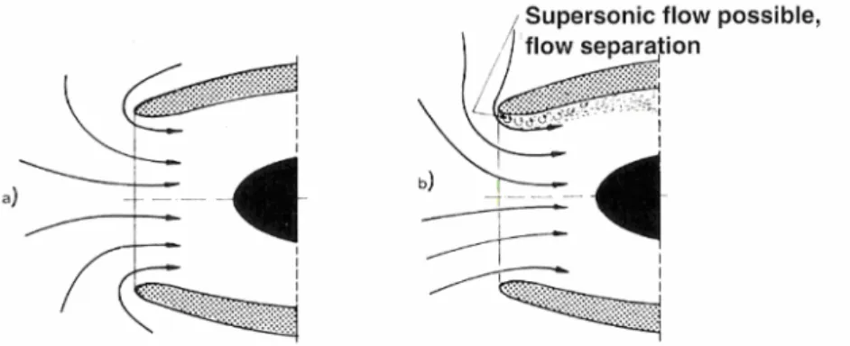
diameter and the free-stream velocity. The area defined by the boundary between the air that enters in the engine and the air that does not is called the intake captured area. The flow ratio and the stream-tube shape vary with the operation conditions of the aircraft engine. In near static configuration since the ambient air is at rest, the engine must accelerate the air using maximum thrust. The extreme local acceleration of the flow at the inlet lip can lead to airflow separation in this region[3]_{, as shown in Figure 3}

b). In cross-wind configuration, the shape of the streamtube is modified near the lip. The cross-flow leads to an increase in the flow velocity near the lip Depending on the strength of the cross-flow, high velocity origins in flow separation leading to a total pressure loss at the engine fan. For strong cross-flow the flow tends to become sonic in the same region.

Figure 3: Intake flowfield in static configuration (a) and when flow separation appears (b).[1]

1.3 Ground Vortices

Overviewing the vorticity principles helps to understand the mechanism that leads to the ground vortex formation and the problems attached to it.

1.3.1 Vortices basics

A vortex is an area of concentrated vorticity. It is also defined by the motion of the fluid swirling rapidly around a center. The speed and rate of rotation of the fluid are greatest at the center, and decrease progressively with distance from the center. The expression of vorticity is dependent on the velocity distribution and is given by the expression:

Or more often written in terms of the rotation vector , with the relation: 2  

The rotation vector is constituted of three components ,   and which represents respectively the rotation about the X axis, the Y axis and the Z axis.

̂    ̂

Corresponding to each rotation terms, the average of angular velocities:

2    2    ̂ ̂

The circulation Γ is the line integral around a closed curve C[4] _{and by using Stokes’s}

law, the vorticity and the circulation are related with the relation:

Γ . .

For a curved surface S, the circulation is the integral of the component of vorticity normal to the surface. In the presence of vorticity and circulation the flow is considered as rotational.

The precise laws of motion that vortices follow were described by Helmholtz. Figure 4 illustrates a vortex line of filament which is everywhere tangent to the vorticity vector. A collection of vortex lines is often called a vortex tube.

The first part of the Helmholtz vortex law states that:

• The vortex line represents a line which is tangent everywhere to the local vorticity vector. On each point of this line . 0 that comes from the divergence theorem wich specifies that the vorticity is divergence free.[4]

• The vortex tube is defined as a set of vortex lines passing through a surface in space.[4] _{Because the two extremity surfaces S}

1 and S2 close the vortex tube and

because the relation . 0 must be satisfied along each vortex line, the circulation at the two end surfaces S1 and S2 are equal. So the circulation along a

vortex tube is constant,

  .[4] (4) (5) (6) (7) (8)

  Figure 4: Vortex line and vortex tube representations.

The second Helmholtz vortex law, was proven by the Kelvin’s theorem that states that the circulation of vortex lines is time independent.

Hence:D

D 0

Vortex lines are compressed if they move through a cylindrical duct with a decreasing area and they are stretched along their axis (Figure 5). Stretching the vortex results in decreasing the radius and consequently increasing the rotational speed to keep the kinetic momentum constant. Moreover, from the relation Γ and because the circulation is constant, it has the consequence of reducing S and thereby increasing the vorticity.

a) Solid body rotating at speed Ω

b) After stretching Ω

> Ω

, since

vorticity per length is conserved.

1.3.2 Core vortex characteristics

The size, defined by the radius and the tangential velocity are two parameters that can be used to describe a vortex. Figure 6 shows that varies along the vortex radius . equals to zero and can be considered as the boundary between the pure rotational flow field which is called the inner part of the vortex and the outer flow.[5]

  Figure 6: Idealization of the tangential velocity inside a tip vortex.[5]

It must also mentioned that the swirl angle is also a relevant feature of the flow and when swirl angle increases, the total pressure distortion also increases.[6]

The models used to describe a vortex are Burges vortex, Lamb-Oseen vortex, Rankine vortex or Vatistas vortex.

1.3.3 Formation of inlet ground vortices

1.3.3.1 Criteria for intake vortex formation

The formation of ground vortices depends on engine power, wind velocity and engine inlet height and size. Previous published works about ground vortices demonstrate that the phenomenon can only occur with the presence of a stagnation streamline between the ground and the intake which is dependent on the velocity ratio ⁄ and the non-dimensional height ⁄ . This stagnation streamline represents the vortex line where

. 0 on each point.

As explained before, in static conditions, the inlet airflow demand increases. The inlet capture surface increases in diameter and starts including the ground to bring the necessary airflow to the fan[7] _{as shown Figure 7. Air flowing into the engine from all}

directions produces a region on the ground surface under the engine in which there is no flow.[8] The streamlines coming from all directions meet in one location where there is no velocity. This specific line is called the stagnation streamline. Figure 7 illustrates this phenomenon.

  Figure 7: Inlet capture surface above the ground.[7]

Typically the formation of ground vortices is characterized by low ⁄  and high

∞

⁄ [8] _{It corresponds to an engine close to the ground operating at a high inlet mass}

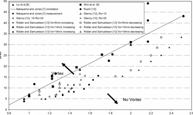
Hence, the mechanism of intake formation is strongly dependant of the height of the engine axis above the ground, the velocity ratio and the presence of upstream velocity. The empirical data was collected by Jermy, M. and Ho. W. H[23] _{and is plotted in Figure}

8.

The velocity ratios / heights combinations that correspond to the appearance of the vortex (or not) are shown in the plot.(Figure 8).

  Figure 8: Data showing the boundary between the vortex forming and non-vortex

forming flow regimes. Where Vi/Vo = / .[23]

An empirical relation also exists for critical velocity ratio at which a vortex first appears.[9]

24 · 17

Figure 8 indicates that a good correlation exists for the occurrence of an intake ground vortex in terms of relative flow rate and the position of the intake. Nevertheless, other parameters as external wind or external vorticity can play a role on the formation of ground vortices.

1.3.3.2 Modes of formation

From previous published works (papers and thesis), it appears that there are four different modes leading to the formation of inlet ground vortices. Other modes of

formation also exist but are combinations of the previous ones that lead to a “non-countable mode”.

1.3.3.2.1 Mode one: Intake with no-wind

A vortex can be generated without ambient wind and with a low ratio ⁄  (in the region of ⁄ < 1). Due to the ground proximity, high levels of suction beneath the engine inlet leads into a strong flow underneath the inlet upstream towards the intake lip.[10] _In

these conditions, it is possible to visualize at the engine intake and at the ground two upward spiralling vortices.

Under no-wind condition, it appears that the two vortices are counter-rotating (Figure 9). In this mode, the vorticity is induced by the boundary layer. Obtaining two counterrotating vortices suggests that the air flowing underneath the engine upstream towards the inlet lip dominates and is stronger than the flow downstream towards the intake lip.

  Figure 9: Sense of rotation of the counter-rotating vortices with no wind.[13]

When the intake vortex formation is dominated by an approaching induced boundary layer the flow structure changes. As shown in Figure 10, (opposite to Figure 9) the sense of the approaching vorticity is clockwise leading to the consequence of inverting the sense of rotation of the intake vortices. The intake vortex rotation sense is highly dependant on of the sense of rotation of the primary vorticity.

  Figure 10: Vortex filament in no-wind mode.[10]

1.3.3.2.2 Mode two: Intake in head-wind

As seen in previous work this mode has been most studied, as shown by Brix[10] with the very detailed and incisive studies in 2000 confirming the results expected by De Sievri et al.[11]

  Figure 11: of rotation of the inlet vortices for a) low, b) medium and c) high

velocity ratios.[13]

Is a head-wind flow, when the air is sucked into the engine inlet, the flow field underneath the intake starts to roll up into two upright counter-rotating vortices (Figure 11 a) ) and a fast flow into the opposite direction of the wind appears between them[10]_.

If the value of the velocity ratio ⁄ ∞ increases and is high enough (approximately 20),

suddenly the sense of rotation of the two vortices switches as illustrated in Figure 11 c). The sense of rotation is then exactly the same as in the no-wind mechanism. In head-wind, the mode dominating the flow field for high velocity ratios (higher than 20) is the mode described previously.

The transition between high and low ratios ⁄ is shown in Figure 11 b). In this phase two pairs of symmetrical vortices rotating in the opposite sense exist together. The phenomenon rarely appears due its very unstable characteristic. If it happens, the two vortices try to cancel each other out and if they do not, one of the two pair of vortex is going to prevail. Nevertheless, the strength of the dominated vortex is very weak. Depending on the velocity ratio, the boundary layer effects are like, as in the no-wind case, stronger on one side than the other. Orientations of the source of vorticity depending on this velocity ratio are shown in Figure 12 and Figure 13.

That change in the sense of rotation can be explained as follows:

At low velocity ratios ⁄ ∞, the upstream flow that flow toward the intake lip generates

an boundary layer smaller compared to the flow flowing underneath the engine downstreaming towards the inlet, as shown in Figure 14

Figure 12: Vortex filaments in head-wind. Mode at high speed velocity ratio.[10]

Figure 13: Vortex filaments in head-wind. Mode at low velocity ratio.[10]

  Figure 14: Reason explaining the sense of rotation of the counter rotating

vortices at low velocity ratio.[13]

At high velocities ratios, the boundary sizes are flipped. The increase in free-stream velocity reduces the size of the upstream boundary layer and the flow flowing upstream towards the intake lip is now in domination as shown in Figure 15.

  Figure 15: Reason explaining the sense of rotation of the counter rotating

vortices at high velocity ratio.[13]

1.3.3.2.3 Mode three: Intake in cross-wind with irrotational flow

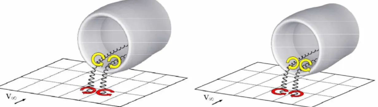
With 90° cross-wind and an irrotational flowfield, two different kinds of vortices appear around the intake: an inlet vortex and a trailing vortex. From the downstream side of the inlet lip region a trailing vortex appears larger in size than the inlet ground vortex. The sense of rotation of these two vortices is represented in Figure 16.

Figure 16: Sense of rotation of the inlet vortex and the trailing vortex.[11]

The variation of flow over the intake in the axial direction causes the formation of the trailing vortex. As the flow moves closer to the inlet, it becomes more three dimensional. The induced velocities caused by the inlet velocity impart additional momentum on the flow around the intake delaying the separation points. Indeed, the induced velocities become higher as one move towards the intake lip thus causing the separation points to be delayed (Figure 17). Separation on the outer surface of the intake appears later near the lip than far from the lip downstream resulting in a higher circulation value at the lip. This presence of circulation leads to the formation of the trailing vortex.

  Figure 17: Separation line around the inlet seen from the top view.[11]

Compared to the previous modes, in upstream irrotational flow, the intake vortex is part of a vortex system. The generation of the circulation along the intake is directly linked to the formation of the trailing vortex system and thus to the intake vortex.

The change in the velocity ratio ⁄ ∞ can also have a significant impact on the

formation of the vortices. At low values of ⁄ ∞ (in the region of <5) the capture

surface does not touch the ground which means no presence of stagnation streamline between the intake and the ground and so no inlet ground vortex. But two counterrotating trailing vortices of equal strength are generated at the rear of the inlet (Figure 18 a) ). The increase in the velocity ratio causes the disappearance of the lower trailing vortex and the formation of the inlet ground vortex (due to increase in the capture area which now includes the ground) as illustrated in Figure 18 b).

Figure 18: Flow aspects for low (<10 say) (a) ; and high (>20) (b) velocity ratios for an inlet in 90° cross-wind with an irrotational upstream flow. [11]

The formation of the inlet ground vortex is dependant on the velocity ratio ⁄ ∞.

An increase in the velocity ratio leads to the transformation of the counter-rotating vortices into an inlet vortex single trailing vortex configuration. And it’s also possible to notice that reducing the height ratio ⁄   has the same consequence as increasing the ratio ⁄ ∞.

a) 

1.3.3.2.4 Mode four: Intake in cross-wind with ambient vorticity

When an engine intake oriented at a 90° yaw angle and with the presence of far upstream vertical vorticity with clockwise rotation, there is the formation of a single clockwise vortex inside the intake. For the same configuration but with a far upstream vorticity having counter-clockwise rotation, a single clockwise vortex is found. The sense of rotation of the vortex is thus opposite to the ambient vorticity and this would not occur if the only mechanism is the amplification of the ambient vorticity.

  Figure 19: Vortex formation in cross-wind with a upstream vertical vorticity.[11]

In Figure 19, there are two vortices shown at the intake. One is very strong near the trailing edge while the other one very weak very close to the other one. The presence of the two vortices with different strength is due to the fact that this mode is a combination of the three previous modes described previously.

Two symmetrical weak counter-rotating vortices have been seen in mode one when there is no-wind. Mode two also generates two vortices but the strength of these vortices is stronger than previously. And in mode three, one strong vortex and one weak vortex are produced.

Intake in tail wind

The results for this configuration are the same as the ones in head-wind.[12]

There is a lack of understandings of these mechanisms, in particular the interaction between them. It is certainly due to a lack of quantitative data of the ground vortex.

2 Mathematical Method

2.1 Introduction

This chapter describes the mathematical model used to obtain a solution of equations of Navier-Stokes that governs the fluid flow simulating an intake in cross-wind with irrotational flow. Section 2.2 and 2.3 presents the governing differential equations based on the turbulence model.[14] _{The section 2.4 and 2.5 are devoted to the solution}

procedure and boundary conditions respectively. The grid study is presented in section 2.6.

2.2 Governing Differential Equations

The time averaged partial differential equations governing the steady, uniform-density isothermal three-dimensional flow may be written in Cartesian coordinates as

and the continuity equation as

    0

where the overbars represent averaged quantities. The turbulent diffusion fluxes are approximated with the high Reynolds number version of the two-equation model described in detail by Launder and Spalding.[14] _{The Reynolds stresses may be}

expressed as

where is the turbulence kinematic viscosity, which is derived from the turbulence model and expressed by

The values for and are obtained by solving the following transport equations:

  (11) (12) (13) (14) (15)

where and are additional dimensionless model constants, and are the turbulent Prandtl numbers for kinetic energy and turbulent dissipation.

The turbulence model constants that are used are those indicated by Lander and Spalding [14]_:

0.09 1.44 1.92 1.0 1.3

Table 1 : Turbulence model constants.

The governing equations constitute a set of coupled partial differential equations that can be written in the general form as

  Γ

X Γ Y Γ Z

Where may stand for any of the velocities, turbulent kinetic energy, or dissipation, and Γ and take on different values for each particular .

2.3 Finite-Difference Equations

The solution of the governing equations were obtained using a finite-difference method that used discretized algebraic equations deduced from the exact differential equations that they represent. This discretization involves the integration of the transport equation over an elementary control volume surrounding a central node with a scalar value (Leonard et al[15]_{), and as far as the convection terms are concerned, it needs the}

spatial average value of at each cell face. The hybrid scheme uses central differencing in obtaining those values when 2 and upwind differencing for 2. In the later case, false diffusion is introduced into the finite-difference equation (e.g. Leonard[16]_{). Erroneous solution may then be obtained in regions of the flow with}

velocity vectors inclined to the numerical grid lines and large diffusive transport normal to flow direction if fine grids are not used, and limit calculation of complex flows. The QUICK scheme proposed by Leonard[16] _{is free from artificial diffusion and gives more}

accurate solutions with grid spacing much larger than required by the hybrid scheme. Due to the use of quadratic upstream-weighted interpolation to calculate the cell values

(16)

for each control volume. Figure 20 shows the west face of a control volume surrounding a central node with a value .

For this face, using a uniform grid for simplicity, the value of is expressed by

If the convective velocity component is assumed to have the direction shown in

Figure 20. If were negative, then would be involved rather than . The first term in the previous equation is the central difference formula, and the second is the important stabilizing upstream- weighted normal curvature contribution. Expressing the values of at each cell face with the appropriate interpolation formula and writing gradients also in terms of node values, the finite-difference equation corresponding to equation 17 may be written in the general form

  ∑ where

  ∑

Here, the summation occurs over the 12 nodes neighbourning (see Figure 21).

  Figure 20: Nodal configuration for the west face of a control volume.[17]

The set of equations for the complete field is solved by the method usually used with hybrid scheme formulation (see Gosman and Pun[18]), but when using QUICK, the coefficients may become negative and stable solutions cannot be obtained. In the present work In the present work, diagonal dominance of the coefficient matrix is

(18)

(19)

ensured and enhanced by rearranging the difference equation for the cell where the coefficients become negative.

This rearrangement consists in subtracting from both sides of equation 19,

eliminating the negative contribution of and simultaneously enhancing the diagonal dominance of the coefficient matrix (Barata et al.[17]_{; Barata et al.}[19]_{; Barata et al.}[20]_;

Silva et al.[21]_).

The source term becomes

where is the latest available value of at node .

Figure 21: Nodal configuration for a control volume.[17]

Therefore, at the present work, the QUICK scheme is used in calculating al variables.

2.4 Solution Procedure

The solution procedure is based on the SIMPLE algorithm widely used and reported in the literature (e.g. Patankar and Spalding[22]_{). It uses the staggered grid arrangement}

and a guess and correct procedure field such that the solution of the momentum equations satisfies continuity.

2.5 Boundary Conditions

The computational domain has six boundaries where dependent values are specified: an inlet plane, a symmetry plane, and two solid walls at the top and side of the channel. On the symmetry plane, the normal velocity vanishes, and the normal derivates of the other variables are zero. At the solid surfaces, the wall function method described in

detail by Launder and Spalding[14] _{is used to prescribe the boundary conditions for the}

velocity and turbulence quantities, assuming that the turbulence is in state of local equilibrium. The domain of the solution is shown in Figure 22.

Figure 22: Domain of the solution a). Representation of the intake with centered referential b).

2.6 Grid independence

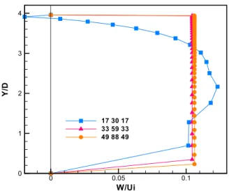
Grid independence tests were performed with different mesh size. The horizontal velocity component, W, is used in Figure 23 to show the grid dependency of the computations. It shows the vertical profiles of the horizontal velocity component, W, at

X/D = 0.53, and plane Z/D =0.035 with different grids. The grid spacing was

non-domain of the solution

Wall 

uniform in all directions. The results were found to be independent of numerical influences with the grids 33 × 59 × 33 and 49 × 88 × 49.

Figure 23: Dimensionless Vertical profile, at X/D=0.53, of the horizontal velocity component, W, at a Z=0.1.

2.7 Summary

This chapter has presented the mathematical model used to study turbulent flows in certain conditions with certain restrictions. A numerical solution for this kind of turbulent flow was obtained from the solution of set of discretized algebraic equations, representatives of momentum (equation 18) and the equations from the turbulent model “ ” and “ ”. When is possible to obtain a convergent solution, the precision is fundamentally a result obtained by the approach method of the convective and diffusive flows in the control volume faces. The use of first-order hybrid difference treatment for the convention terms can cause problems in allowing false diffusion errors to present grid independence achieved in reasonable meshes and, thus, masking the true performance of the turbulence model. For that, the quadratic upstream interpolation QUICK method used in the present study makes possible obtaining the same numerical precision with coarse grids. And finally the grid independence study was presented. W/Ui Y/ D 0 0.05 0.1 0 1 2 3 4 17 30 17 33 59 33 49 88 49

3 Results

3.1 Introduction

Numerical prediction of cross-wind mode was obtained using the computational method described in section 2. In this chapter, the effect of the non-dimensional height, the effect of the non-dimensional velocity and three ⁄ with equal / were studied

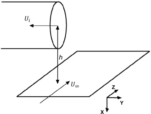
3.2 Geometry Model

To investigate the effects of ground vortices, the intake represents a 1/1th _{scale model}

with a diameter of 2.83m which correspond to the engine Trent 900 with no eccentricity. Figure 24 shows the configuration. In table 1 the test case conditions are summarized.

  Figure 24: Configuration used in the Test-Case simulation.  

  Cross‐Wind Simulation 

/   0.97 

(kg/s)  84.77 

⁄   9.9 

Table 2 : Test-Case conditions.

h

X

Y Z

3.3 Effect of the Height of the Intake

Increasing or decreasing the height of the intake has a significant impact on the vortex characteristics. The first difference is that the vortex increases in size with the reduction in the ground clearance. When the ground is closer to the intake the air drawn in between the ground and the intake (called “gap flow”) reduces, causing more air to be sucked in from above. So as the ground clearance increases the gap flow gets higher and so the vortex location on the ground moves away from the intake plane until it disappears. To demonstrate the effect of the non-dimensional height influence, three ⁄  configurations have been studied Figure 25 shows the results for ⁄  0.97 (a), ⁄   1.02 (b) and ⁄   1.20 (c). The results are represented for all the conditions in the plane facing the intake on a Y plane Y=Ymax.

Figure 25 Flow patterns for ⁄ equal to 0.97 (a), 1.02 (b), and 1.20 (c) in the plane facing the intake on a Y plane Y=Ymax.

From Figure 25 a), for ⁄ 0.97, two recirculation zones can be observed. As long as the height changes, the flow changes dramatically. In the Figure 25 b), for

Z/D Y/ D 0 2 4 6 0 0.5 1 1.5 2 2.5 Z/D X/ D 0 1 2 3 4 5 6 7 0 0.2 0.4 0.6 0.8 Z/D X/ D 0 0.5 1 1.5 2 2.5 3 3.5 4 4.5 5 5.5 6 6.5 7 0 0.2 0.4 0.6 0.8 1 Z/D Y/ D 0 1 2 3 4 5 6 7 0 0.5 1 1.5 2 2.5 3 Z/D X/ D 0 0.5 1 1.5 2 2.5 3 3.5 4 4.5 5 5.5 6 6.5 7 0 0.2 0.4 0.6 0.8 1 1.2 a) b) c)

⁄   1.02, the flow that is sucked directly from the ground to the intake is located far upstream and with lower intensity than in the configuration with lower height. In the Figure 25 c), for ⁄   1.2 which is the configuration with the greatest height, the ground flow cannot reach the intake and so it flows upstream influenced by the neighbor layers.

3.4 Effect of the Cross-Flow Velocity,

Increasing or decreasing the cross-flow velocity, ∞, together with the engine height

(h), has a significant impact of the vortex formation and location. Figure 26 shows the flow patterns for   ⁄  equal to 9.9 (a), 9.4 (b), and 8.7 (c) at X=2.75.

Figure 26: Flow patterns for ⁄  equal to 9.9 (a), 9.4 (b), and 8.7 (c) at X=2.75.

The decrease of the velocity ratio between the intake and the crossflow corresponds to a recirculation moving away from the intake. When the velocity ratio decreases from 9.9 to 9.4, Figures 26 a) and b), the recirculation moved further downstream and became larger with lower intensity. With a further decrease of the velocity ratio the recirculation disappears completely. As shown in Figure 26 c) the lowest velocity ratio   ⁄ Z/D X/ D 0 1 2 3 4 5 6 7 0 0.2 0.4 0.6 0.8 Z/D Y/ D 0 1 2 3 4 5 6 7 0 1 2 3 Z/D Y/ D 0 1 2 3 4 5 6 7 0 1 2 3 Z/D Y/ D 0 1 2 3 4 5 6 7 0 1 2 3 a) b) c)

3.5 Results from the cross-wind test case,

⁄

.

Figure 27 shows the flow pattern for / 0.97 and / 9.9. The velocity vectors are represented together with W velocity contours in three different planes. In figure 27 a) two horizontal planes ( /  1.76 and 3.72), and one vertical plane ( / 0.33). The vertical plane shows a large region of negative values of W which indicates a strong flow in the opposite direction of the crossflow. In figure 27 b) two vertical planes ( / 1.75 and 5.17), and one horizontal plane ( / 1.76). The vertical plane ( / 5.17 ) and the horizontal plane as Figure 27 a) confirms a strong flow in the opposite direction of the crossflow. In general the flow is in the direction of the intake which located at Z=10m, and Y=h. The negative values of W indicate a flow pattern of the type shown in Figures 25 a) and 26 a) which corresponds to a eccentrical flow type.         0 5 10

Y

X

Z

a)

  Figure 27 : Flow pattern and isolines of W for / . and / . .  

Figure 28 shows isolines of U,V and k in the vertical plane of symmetry at X=0. These results confirm the conclusions drawn from Fig. 27 with large positive (upwards) values of the vertical velocity component near the axis of the engine intake (Z/D=3.5). The highest values of the turbulent kinetic energy are observed in the downstream side (in the Z direction) of the flow.

0 5 10

Y

X

Z

a)

b)

  Figure 28 : Isolines of U,V and k in the vertical plane of symmetry at

X=0 ( / =0.97, and / =9.9).  

Figure 29 shows isolines of U, V, W and k in the vertical plane which contains the the engine axis (at Z=Zmax/2), and perpendicular to the crossflow. These results showed

that closer to the engine axis, the values of U, V, W and k were stronger. Figure 29 b) which represents the isolines of V, showed that at the engine axis plane (Z=Zmax/2)

could be found two zones with pronounced negative velocities. Z/D Y/ D 0 1 2 3 4 5 6 7 0 1 2 3 V 2 1.5 1 0.5 0 -0.5 -1 -1.5 -2

b)

c)

Figure 29: Isolines of U,V, W and k in the vertical plane which contains the the engine axis (at Z=Zmax/2), and perpendicular to the crossflow ( / =0.97, and

/ =9.9). X/D Y/ D 0 0.25 0.5 0.75 0 0.5 1 1.5 2 2.5 3 3.5 _2.5U 2 1 0.5 0 -0.5 -1 -2 X/D Y/ D 0 0.25 0.5 0.75 0 0.5 1 1.5 2 2.5 3 3.5 _2.5V 2 1 0.5 0 -0.5 -1 -2 X/D Y/ D 0 0.25 0.5 0.75 0 0.5 1 1.5 2 2.5 3 3.5 _2.5W 2 1.5 1 0 -0.5 -1 X/D Y/ D 0 0.25 0.5 0.75 0 1 2 3 k 40 35 30 25 20 15 10 5 0 -5

b)

a)

c)

d)

Parallel ground planes also have been studied. Figure 30 a) shows the Pressure in ground plane, X=h, Figure 30 b) shows the Pressure between the intake and the ground, X=h/2, and Figure 30 c) shows Pressure at the axis of the engine intake, at X=0.

  Figure 30 : Isolines of pressure in (a) ground plane, X=h, (b) plane parallel to the axis intake and the ground, X=h/2, and (c) plane containing the axis of the intake,

X=0, ( / =0.97, and / =9.9).       Z/D Y/ D 0 1 2 3 4 5 6 7 0 1 2 3 P 500 375 125 0 -50 -125 -250 -375 -500

a)

b)

c)

Figure 30 shows that the pressure decreases when approaching the axis of the engine intake (X=0). Figure 30 c) reveals the presence of negative pressure, indicating some vorticity effect.

Figure 31 sustains the conclusions drawn from Figure 30 and demonstrates a 3D particle visualization showing the formation and location of a vortice at the same place of negative pressure, P, in Figure 30 c).

a)

  Figure 31 : 3D particle visualization showing the formation and location of a

vortice ( / =0.97, and / =9.9).

5 Conclusions

This section presents the more important results and findings of the present work. Computational Fluid Method tools have been applied to predict and understand ground vortices forming between the ground and a 1/1th _{scale model intake of a engine.}

Calculations have been performed under cross-wind ground vortice mode of formation. The effect of the height of the intake to the ground and the effect of the cross-flow velocity have been studied in term of velocities and turbulent kinetic energy. The cross-flow velocity test-case was made for / 0.97, and / 9.9 and showed the formation of one vortice at an upstream location. The study of the effect of cross-flow velocity and the effect of the height of the intake showed that are fulcral parameters for the appearance and strength of the vortice.

Recommendations for further work

Only one configuration has been studied under one mode of ground vortice formation. It would be very interesting to determinate ground vortice characteristics for more configurations to obtain a more detail set of data on the ground vortice.

6 References

[1] Yadlin, Y. “Simulation of Vortex Flows for Airplanes in Ground operations”, AIAA Paper 2006-56, 2006

[2] Hünecke, K. “Jet Engines: Fundamental of theory, design and operation”, UK: Airlife publishing, 1997

[3] Mattingly, J. “Elements of Gas Turbine Propulsion”, Singapore: McGraw-Hill, 1996

[4] Green, S. “Fluid Vortices: Fluid Mechanics and its Applications”, Vol. 30, Kluwer Academic Publishers, 1995

[5] Leishman, J. “Principles of Helicopter Aerodynamics”, Cambridge University Press, 2000

[6] Seddon, J. & Goldsmith, E. “Intake Aerodynamics”, Blackwell science, 1985

[7] Johns, C. “The Aircraft Engine Inlet Vortex Problem”, AIAA’s Aircraft Technology, Integrations and Operations (ATIO) 2002 Technical, 1-3rd 2002, Los Angles, California, AIAA 2002-5894

[8] Swainston, M. “Vortex Formation Near Intakes to Turbomachinery and Duct Systems”, Heat and Fluid Flow, Vol. 4, No. 2, 1974

[9] Nakayama, A. & Jones, J. “Correlation for Formation of Inlet Formation”, AIAA Journal, Vol. 37, No. 4: Technical Notes, 1998

[10] Brix, S., Neuwerth, G. & Jacob, D. “The Inlet-Vortex System of Jet Engines Operating Near the Ground”, AIAA Paper 2000-3998, 2000

[11] De Siervi, F., Viguier, H., Greitzer, E. & Tan, C. “Mechanisms of Inlet Vortex Formation”, J. Fluid Mech., Vol. 124, pp. 173-207, 1982

[12] Motycka, D. & Walter, W. “An Experimental Investigation of Ground Vortex Formation During Reverse Thrust Operation”, AIAA Paper No. 75/1322, AIAA/SAE 11th Propulsion Conference, 1975

[13] Rehby, L. “Jet Engine Ground Vortex Studies”, MSc Aerodynamics , Crandfield University, 2007

[14] Launder, B. E. and Spalding, D. B. "The Numerical Computation of Turbulent Flows", Computer Methods in Applied Mechanics and Engineering, Vol. 3, No. 2, pp. 269-289, 1974.

[15] Leonard, B. P., Leschziner, M. A., and McGuirk, J. J. “Third-Order Finite-Difference Method for Steady Two-Dimensional Convection”, Procedings of the 1st _{International}

Conference on Numerical Methods in Laminar and Turbulent Flow, edited by C. Taylor et al., Pentech Press, London 1978

[16] Leonard, B. P. “A Stable and Accurate Convective Modelling Procedure Based on Quadratic Upstream Interpolation”, Computer Methods in Applied Mechanics and Engineering, Vol. 19, No.1, pp. 59-98, 1979

[17] Barata, J. M. M., Durão, D. F. G., McGuirk, J. J. “ Numerical Study of Single Impinging Jets Through a Crossflow”, Journal Of Aircraft, Vol. 26, pp. 1002-1008, 1989

[18].Gosman, A. D. and Pun, W. M. “Calculation of Recirculating Flows”, Imperial College Ret. HTS/74/2, Imperial College, London, 1974

[19] Barata, J. M. M., Cometti, A., Mendes, A. and Silva, A. R. R. "Numerical Simulation of an Array of Droplets Through a Crossflow", AIAA paper 2002-0872, 40th AIAA

Aerospace Sciences Meeting and Exhibit, Reno, Nevada, 14-17 January 2002a.

[20] Barata, J. M. M., Cometti, A., Mendes, A. and Silva, "Numerical Simulation of an Array of Droplets Through a Crossflow", AIAA Meeting Paper on Disc, Reno, Nevada, ISSN 1087-7215, ISBN 1-56347-532-4, 2002b.

[21] Silva, A. R. R., Mendes, A., Cometti, A. and Barata, J. M. M., "Numerical Studies of biphasic tridimensional Flows", V Congresso de Métodos Numéricos en

[22] Patankar, S. V. and Spalding, D. B. "A Calculation Procedure for Heat, Mass and Momentum Transfer in Three- Dimensional Parabolic Flows", International Journal of

Heat and Mass Transfer, Vol. 15, No. 10, pp. 1787-1805, 1972.

[23] Jermy, M. and Ho. W. H. “Location of the vortex formation threshold at suction inlets near ground planes by computational fluid dynamics simulation”, Department ofMechanical Engineering, University of Canterbury, Christchurch, New Zealand, July, 2008