Topology optimization applied to 2D elasticity problems considering the geometrical nonlinearity

Topology optimization applied to 2D elasticity problems considering the

geometrical nonlinearity

Walliston S. Fernandes

a

, Valério S. Almeida

b,⇑

_{, Francisco A. Neves}

c

_{, Marcelo Greco}

a a_{Graduate Program in Structural Engineering, Department of Structural Engineering, Federal University of Minas Gerais (UFMG), Brazil} b_{Department of Geotechnical and Structural Engineering, School of Engineering, University of São Paulo, Brazil}

c_{Department of Civil Engineering, Federal University of Ouro Preto (UFOP), Brazil}

a r t i c l e

i n f o

Article history:

Received 16 September 2014 Revised 25 May 2015 Accepted 26 May 2015 Available online 19 June 2015

Keywords:

Topological optimization Geometrical nonlinearities Evolutionary heuristic formulation Finite element method

a b s t r a c t

Topological Optimization (TO) of structures in plane stress state with material elastic-linear behavior, but taking into consideration the geometrical nonlinearities, was performed and the results are presented herein. For this process, an evolutionary heuristic formulation denominated SESO (Smoothing Evolutionary Structural Optimization) associated with a finite element method was applied. SESO is a variant of the classic evolutionary structural optimization (ESO) method, where a smoothing process is applied in the ‘‘hard-kill’’ process of element removal – that is, their removal is done smoothly, reducing the values of the constitutive matrix of the element as if it were in the process of damage. It has been demonstrated that this non-linear geometric phenomenon clearly influences the final optimized topology when compared to an optimum configuration obtained with the equilibrium equations written at an undeformed position. Some numerical examples from literature are presented in order to show the differences in the final optimal topology when linear and non-linear analyses are used, allowing the verification of the importance of correctly analyzing the final optimum topology and as such, demonstrate the advantages of SESO as a structural optimization method.

Ó2015 Elsevier Ltd. All rights reserved.

1. Introduction

The optimizing process aims to find a suitable model, according to one or more cost criteria, so that certain design constraints can be minimized or maximized. It can involve a different production methodology in an industrial plant, aiming to improve production within less time or to reduce the cost of a product to replace a cer-tain type of constitutive material. In the structural design field, it can be stated that optimization is the search for a better model to meet a specific project request.

Optimization can be divided into three types: parametric, where the structure presents a fixed shape and topology and varies (optimizes) only in constitutive materials used and/or the dimen-sions of the structural elements [1]; shape, where the structure presents a fixed topology, varying its shape and not having hole insertions; in other words, the design variables define the bound-ary of the domain whose shape is altering during the optimization process [2]; and topological, which is a generalization of other

optimization modes, since in this case, the insertion of holes in the initial domain is permitted and the initial boundary can be eliminated [3]. Regarding the methods of optimization, according to[4], they can be classified as: Density approach (such as SIMP), Topological derivatives, Level set approach (for example, Hamilton–Jacobi equation), Phase field approach and Evolutionary approaches (such as ESO/BESO/SESO), the latter being considered as Discrete approaches, of which one (the SESO – Smooth Evolutionary Structural Optimization approach) was adopted in the method used in this work.

According to[5], when compared to the large amount of publi-cations regarding small displacement topology optimization for-mulation, very few research works have been done on large displacements optimization field. Thus, the authors applied con-cepts of optimization considering geometrical nonlinear analysis under full loads using compliance as the objective function. The sensitivity of the mean compliance, since the optimization was accomplished by a gradient-based approach, used the adjoint method to calculate the derivatives.

Furthermore, according to[6], when a very large load is applied or structural deformation is also very large, material or geometrical nonlinearity, or both, may occur due to mechanical conditions. In order to obtain a more useful and valuable optimal structural

http://dx.doi.org/10.1016/j.engstruct.2015.05.042

0141-0296/Ó2015 Elsevier Ltd. All rights reserved.

⇑Corresponding author.

E-mail addresses:walliston@dees.ufmg.br(W.S. Fernandes),valerio.almeida@ pq.cnpq.br(V.S. Almeida),fassis@em.ufop.br (F.A. Neves),mgreco@dees.ufmg.br

(M. Greco).

Contents lists available atScienceDirect

Engineering Structures

topology, satisfying the given constraints, the above nonlinearities should be considered in analysis and design. To carry out the non-linear optimization problem, a modified algorithm based on the ant colony optimization algorithm was applied by the authors [6], but the search procedure is still not simple in terms of numer-ical implementation.

Applying the procedures performed by [5,6]led to numerical manipulation in the finite element analysis program, and insertion of more sophisticated mechanical models, such as dynamic, elasto-plasticity, and non-linear geometric analyses, requiring more com-plex algorithms which need to be altered. SESO is a method that can easily be applied for a commercial program, since it evaluates the macroscopic part of each domain. The formulation presented in [7] for topology optimization of linear plane problems demon-strated to be a fast, reliable and robust optimization and it is there-fore extended herein in the context of geometric nonlinear analysis. In order to verify the effects of geometric nonlinearity in the final topology, some examples are run with the SESO algo-rithm. The results show that the consideration of this kind of non-linear effect leads to a distinct topological configuration from that obtained with linear models. This demonstrates that a geo-metric nonlinear analysis is indispensable for the topological opti-mization process of structures undergoing large displacements.

The algorithm to solve topology optimization problems for geo-metrically nonlinear structures is illustrated using a flowchart (Fig. 4) and could easily be extended to others finite element mod-els incorporating more complex phenomena related to material or dynamic behavior.

2. Smoothing evolutionary structural optimization (SESO)

SESO consists of a gradual removal of finite elements previously generated, in regions that do not effectively contribute to the struc-ture (‘‘inefficient materials’’) by any of the criterion for rejection. This is a variant of the ESO (Evolutionary Structural Optimization) method that was developed by[8]. The authors pre-sent a method dedicated to perform modifications on the topology of a structure, in a simple way, using a heuristic (approximated) technique that gradually removes finite elements corresponding to the regions that do not effectively contribute to a better perfor-mance of the structural system.

Therefore, the entire structure is discretized with a fixed finite element mesh, also named design or extended domain, that

includes the boundary conditions (forces, displacements, cavities and other initial conditions) of the elastic problem to be solved iteratively via FEM. Afterwards, the principal stress is evaluated at each element, and the highest stress value of the whole struc-ture, the maximum von Mises stress, is taken as reference to be used in inequality(1a), as described in[7].

r

vm

e <RRk

r

vm

i;max ð1aÞ

RRkþ1¼RRkþER ð1bÞ

where

r

vm

e is the equivalent von Mises stress of thei-th element in the iteration and

r

vm

i;maxis the maximum effective stress of the struc-ture in the iteration ‘‘i’’;RRkis the Rejection Ratio at the k-th steady state (0.06RRk61.0), which is an input parameter that is updated using the Evolution Rate (ER). The evolutionary process is defined by adding the evolution rate to the Rejection Rate, presented in Eq. (1b), which is applied to control the removal process of the structure.

Hence, the elements that satisfy Eq.(1a)are gradually removed in the mesh by an iterative process until a steady state is achieved. This removal is done by altering the constitutive matrix, for exam-ple, by setting a very small value to that element’s stiffness (for instanceD= 1012_{), which makes this element inefficient without}

the need to remake the mesh of the problem.

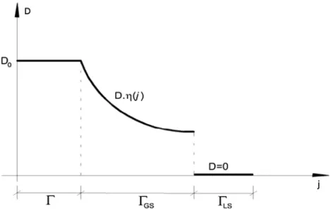
However, just the removal of the elements in the iteration, according to Eq.(1a), can often leads to an early or precipitated withdrawal of elements that should not be removed. This happens often due to the fact that during the evolutionary process a certain element that should not have been taken out was removed just to reach this equation. The generated solution is forced, non-optimal and possibly generates an unstable region called ‘‘chessboard’’ (or ‘‘checkerboard’’), considered to be one of the major problems in topological optimization. To solve this problem, SESO proposes an organization of elements that does not satisfy Eq.(1a)such that (p%) of these elements are removed and (1p%) is are returned to the structure. This return is accomplished by a regulating function that performs a smoothing procedure or, in other words, it weights elements with a higher potential for removal and removed ele-ments that can be returned to the mesh. This procedure can mini-mize, or even eliminate, the ‘‘chessboard’’ because the voids of possible unstable regions are returned due to their neighbors. This procedure can be interpreted as follows:

DiðjÞ ¼

D0; if j2

C

i D0

g

jð

C

Þ; if j2

C

GS

0; if j2

C

LS

8 > < > : 9 > = > ;

ð2Þ

whereC¼CLSiþCGSi,CLSiis the domain of elements that should be

effectively excluded, CGSi the domain of elements which will be

returned to structure, for 06

g

ðCÞ61 is the regulating function that weights the value of the rate

r

vm

e =r vm

maxwithin theCdomain, and this procedure can eliminate the checkerboard problem.

The proposed smoothing can be, for example, performed by

g

ðCÞusing a linear function of the

g

ðCÞ ¼

a

jþbtype or a trigono-metric function of the

g

ðCÞ ¼sinð

a

jÞtype. Because these two func-tions are continuous, they can be differentiated over all the C

domain, and they have an image varying from 0 to 1, Fig. 1. Nonetheless, here the trigonometric function was used to weight theCGSdomain. It is noteworthy that for smaller values of the ele-ment removal ratio used by the SESO optimization criterion, the more accurate the final design is, the more expensive it becomes because of greater computational time.

In addition, SESO also proposes a stopping criterion for element removal. The Performance Index (PI) is a dimensionless parameter that measures the efficiency of structural performance. Therefore, from the expression proposed by[9]and the smoothing generated by Eq.(3)that modifies the constitutive matrix in terms of struc-tural thickness due to a direct linear relationship, the Performance Index, as demonstrated by [7], can be written as follows:

PI¼

r

VM 0;max

r

VM

i;max !

_PA_NE0t

j¼1Ajtj

¼

r

VM 0;max

r

VM

i;max !

_PNEA0t0

j¼1Ajtj

g

ðjÞ

ð3Þ

wheret0is the initial thickness andtjis the thickness of thejth ele-ment at thei-th iteration. Thus, the definition of the optimal topol-ogy is verified by this performance index, which is a factor of monitoring the structural performance. If this rate falls sharply, it is a strong indication that it exceeded a possible ideal or stationary configuration. However, there is no guarantee that this is the global optimum topology, but rather an ideal setup for an engineering design.

In terms of removal criteria for geometrical nonlinear problems, some authors such as[10–13]use mean compliance as the objec-tive function to remove elements. The proposal of the present paper is to adopt a simpler criterion, regarding the computational implementation that guarantees acceptable results when com-pared to the results obtained from other techniques found in the literature. Thus, the methodology presented in Simonetti et al. [14], originally used for the optimization of linear structures, is applied here for the optimization of geometrical nonlinear struc-tures. Moreover, the proposed geometrical nonlinear formulation (positional) is also different from the usual nonlinear formulations. It is an original approach that presents good results when com-pared to the literature. Another advantage of the proposed method is that it can be extended to optimization of dynamic problems. The negative effect is the maximum stress values that can occur during the removal process, as the inequality that governs the problem, Eq.(1a), is entirely dependent on the maximum stress

of the structure. That is, the maximum stress caused by the redis-tribution of the stress field can be inappropriate for larger topolo-gies or for the case of slender structures. To minimize this problem, a filter was applied, with it consists in using an average value of stress considering the top ten stress values.

3. The adopted nonlinear finite elements approach

The formulation used in this article is based on the principle of stationary total potential energy of a structural system in equilib-rium. The equilibrium position is related to a non-linear problem and the Newton–Raphson method is used for iterative processing of the displacement calculations. Of all the possible configurations in a flexible structure system with its actuating forces, that which corresponds to the maximum (or minimum) value of the total potentialPis the equilibrium configuration. The total potential energy,P, is the sum of the total strain energy,Ut, and the poten-tial energy of the total external forces,P¼P

FX, in the analyzed initial structural volumeV[15]. The energy functionPis given by:

P

¼UP ð4Þ

where U¼ Z V udV¼ Z V Z e

r

d

e

dV ð5Þ

The specific strain energy, or strain energy by unit of volume, can be written in matrix form as follows:

u¼1

2

r

T

_e

_ð6Þ

For the case of a plane stress state the specific strain energy can be written as follows:

u¼1

2 c11e

2

Xþc22

e

2Yþc44c 2 XY

þ1

2ð2c12eX

e

Yþ2c14cXY

e

Xþ2c24cXY

e

YÞ ð7Þ

With the aim of developing a numerical method in accordance with[15], Eq.(4)was minimized for the energy function.

@

P

@X¼ Z

V

@u

@XdVF¼0 ð8Þ

It is important to observe the non-linear nature of Eq. (8), becauseu¼uð

e

X;

e

Y;

c

XYÞ. The variable (X) represents nodal posi-tions, horizontal as well as vertical. In reality, Eq.(8)represents a set of non-linear equilibrium equations for each nodal position. The solution for the set of equations represented by(8)is the equi-librium of the structure in the deformed position for maximum and

Table 1

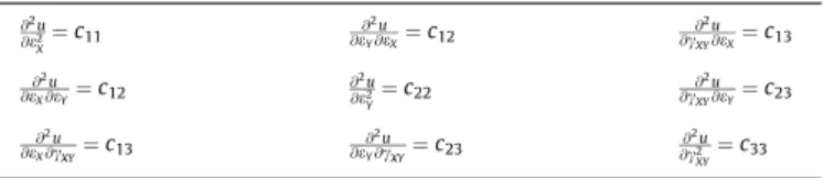
Second derivatives for specific strain energy.

@2_u @e2

X¼c11

@2_u @eY@eX¼c12

@2_u @cXY@eX¼c13

@2_u @eX@eY¼c12

@2_u @e2

Y¼

c22 @

2_u @cXY@eY¼c23

@2_u @eX@cXY¼c13

@2_u @eY@cXY¼c23

@2_u @c2

XY¼c33

minimum energy conditions and can be solved directly by algo-rithms of Quasi-Newton type, where the iterative process includes only the vectors related to the external forces applied and the internal equilibrium forces of the nonlinear problem to achieve the equilibrium position. The most stable strategy is the solution of the equations by algorithms of the Newton–Raphson procedure. Consider that there is a nonlinear function represented in Eq.(9), whose residual vector (gðXÞ) in the equilibrium position is zero.

gðXÞ ¼

Z

V

@u

@XdVF¼0 ð9Þ

Then the function gðXÞ is linearized by a first order Taylor expansion, whose solution is performed via an iterative search pro-cedure. Purposely considering the first order Taylor expansion, an approximation error is introduced that will be compensated by the iterative algorithm:

0¼gðXÞ ¼gðX0Þ þ

r

gðX0Þ

D

X ð10Þ

Eq.(10)is used to calculate the deformed positions in nonlinear equilibrium.

r

gðX0Þ

D

X¼ gðX0Þ ð11Þ

The gradient of the residues functiongðXÞis the Hessian matrix

rgðX0Þof the problem. The vector for the residuals is calculated

based on Eq.(9).

The first derivatives for the specific strain energy in relation to the nodal positions are integrated into the volume according to Eq. (9), and it can be developed according to the chain rule:

@u

@Xi

¼@u @

e

X

@

e

X

@Xi

þ@u @

e

Y

@

e

Y

@Xi

þ @u @

c

XY

@

c

XY

@Xi

ð12Þ

The specific strain energy derivatives in relation to the (deformed) components are calculated according to Eq.(7).

@u

@

e

X

¼c11

e

Xþc12eYþc14cXY ð13Þ

@u

@

e

Y

¼c22

e

Yþc12eXþc24cXY ð14Þ

@u

@

c

XY

¼c44cXYþc14eXþc24eY ð15Þ

The second derivatives for specific strain energy in relation to the strain components that were utilized to calculate the Hessian matrix are presented inTable 1. The second strain derivatives for specific strain energy in relation to the nodal positions are inte-grated in the volume for the Hessian matrix calculation and it can be developed according to the following chain rule:

@2u

@Xj@Xi¼

@ @Xj

@u

@Xi

¼ @

@Xj

@u

@

e

X

@

e

X

@Xiþ

@u

@

e

Y

@

e

Y

@Xiþ

@u

@

c

XY

@

c

XY

@Xi

ð16aÞ

r

gðXÞ ¼

Z

V

@2u

@Xj@Xi

dV ð16bÞ

where

@ @Xj

@u

@

e

X

@

e

X

@Xi

¼ @

@Xj

@u

@

e

X _@

_e

X

@Xi

þ@u @

e

X

@ @Xj

@

e

X

@Xi

¼ @

2 u

@Xj@

e

X

@

e

X

@Xi

þ@u @

e

X

@2

e

X

@Xj@Xi

¼ @

2_u

@

e

2 X

@

e

X

@Xj

þ @

2_u

@

e

X@

e

Y

@

e

Y

@Xj

þ @

2_u

@

e

X@

c

XY

@

c

XY

@Xj !

@

e

X

@Xi

þ@u @

e

X

@2

e

X

@Xj@Xi

ð17Þ @ @Xj

@u

@

e

Y

@

e

Y

@Xi

¼ @

@Xj

@u

@

e

Y _@

_e

Y

@Xi

þ@u @

e

Y

@ @Xj

@

e

Y

@Xi

¼ @

2_u

@Xj@

e

Y

@

e

Y

@Xi

þ@u @

e

Y

@2

e

Y

@Xj@Xi

¼ @

2_u

@

e

Y@

e

X

@

e

X

@Xjþ

@2u

@2

e

Y

@

e

Y

@Xjþ

@2u

@

e

Y@

c

XY

@

c

XY

@Xj !

@

e

Y

@Xi

þ@u @

e

Y

@2

e

Y

@Xj@Xi ð

18Þ

@ @Xj

@u

@

c

XY

@

c

XY

@Xi

¼ @

@Xj

@u

@

c

XY

@

c

XY

@Xi

þ @u

@

c

XY

@ @Xj

@

c

XY

@Xi

¼ @

2 u

@Xj@

c

XY

@

c

XY

@Xi

þ @u

@

c

XY

@2

c

XY

@Xj@Xi

¼ @

2_u

@

c

XY@

e

X

@

e

X

@Xj

þ @

2_u

@

c

XY@

e

Y

@

e

Y

@Xj

þ@

2_u

@

c

2 XY

@

c

XY

@Xj !

@

c

XY

@Xi

þ @u

@

c

XY

@2

c

XY

@Xj@Xi

ð19Þ

Thus, the Newton–Raphson iterative process is summarized as follows:

Assume X0 as the initial configuration (non-deformed).

Compute the vector of residuesgðX0Þthrough Eq.(9);

Find the Hessian matrixrgðX0Þthrough Eq.(16b);

Solve the system defined in Eq.(11)to findDX;

Update nodal positions:X¼X0þDX. Return to step 1 untilDX

is sufficiently small.

The finite element utilized to solve the nonlinear system is the Quadratic Strain Triangle (QST), being that the element in study is of triangular geometry with a total of 10 nodes, according toFig. 2. The non-dimensional parametersn1,n2andn3are the

homoge-neous coordinates of the triangular element (or triangular coordi-nates) given byn3¼1n1n2.

The displacements distributions are expressed as complete cubic. To satisfy the displacement compatibility between the ele-ments, the displacement function should only depend on the dis-placement of the nodes of the side in question. As the function is cubic, four nodes per face of the element are necessary, together with one node in its interior. This node is necessary to maintain the integrity of the polynomial, since if the polynomial is not com-plete, the rigidity will have an undesirable direction. Besides this, the node should be preferentially in the centroid of the element [16]. The QST is not an isoparametrical element, but it has good approximation for the stress and strain fields.

The numerical integrationsR

V @ u

@XidV and rgðX0Þ ¼

R

V @

2_u @Xj@XidV,

presented in Eqs. (20) and (21), are calculated using 7 Hammer points per finite element.

Z

V

@u

@Xi

dV¼X

7

g¼1

@uðn;XiÞ

@Xi

x

gdetðA0ðngÞÞ ð20Þ

r

gðX0Þ ¼ Z

V

@2u

@Xj@Xi

dV¼X

7

g¼1

@2uðn;XiÞ

@Xj@Xi

x

gdetðA0ðngÞÞ ð21Þ

4. Topology optimization applied to geometrical nonlinear problems

When considering geometric imperfections or large configura-tion changes in structural analyzes, there are no longer linear

relation between displacements and applied forces. The change in geometry, compared to a preset initial configuration, may be due to an error in the manufacturing of the structural part, due to a mounting error of the material according to its purpose or due to displacements and rotations of the original setting by any load. When the structure undergoes large displacements according to the load applied, problems can appear from struc-tural instability and internal forces that are not initially foreseen will appear too. Thus, a geometric nonlinear analysis is necessary.

The nonlinear analysis must be taken into account during the topology optimization process in order to influence on the stress flux developed in the structure and consequently on the optimal topology configuration.

According to the flowchart below (Fig. 3), in order to obtain the optimum topology, the elements are removed by respecting an established stop criterion (Performance Index or Maximum Volume). The element removal criterion presented herein was per-formed using stresses, or in other words, the elements that have values lower than the maximum active stress are removed. In this sense, whether it is a linear or a nonlinear analysis, that optimizer only removes the elements that do not satisfy the preset stress cri-terion. Still, it is interesting and important to observe that the opti-mum models for linear and nonlinear analysis are not always behaves in the same manner. This is due to the difference in the stress distribution of the finite elements along the iterations that remove these elements and also due to the nonlinear nature of some structures, depending on the geometry and conditions of the initial boundaries.

After ending all load steps, an analysis of the von Mises Stress of the element and Maximum von Mises Stress of the structure is per-formed in order to define the elements to be removed. Further, the next optimization iteration is performed.

5. Numerical examples

The results from the linear and nonlinear modeling are now presented. In the unmentioned cases, the linear results were obtained by the formulation presented in[7], where not only the finite element with 9 degrees of freedom, three at each vertex of the triangle, but also all formulation is distinct from the one previ-ously shown.

For the nonlinear case, the algorithm was implemented using the Fortran 90 programming language (compiled using Compaq Visual Fortran v6.6 environment) by authorship of the authors of the manuscript. The solver used for iterative Newton–Raphson procedure is the free subroutine MA27 by HSL Mathematical Software Library. To generate DXF images along optimization steps, the free source routines DXFortran were used. The same rou-tines were used for the linear case. But the main difference for the linear case, besides the formulation, is the absence of the Newton– Raphson procedure.

For the first three numerical examples, analyses were per-formed and depicted through curves load versus displacement dur-ing the iterative optimization process.

The variation of maximum von Mises stress and displacement versus iteration during the optimization process is illustrated graphically. These elements and nodes monitored are located at the same position where the load is applied. For the last numerical example, a displacement evolution, regarding the upper-right node, is shown. For numerical analyses, a simpler membrane finite element has been used.

In the nonlinear analyses for the optimum topology and its respective displacements, the total load is applied in ten incremen-tal load steps.

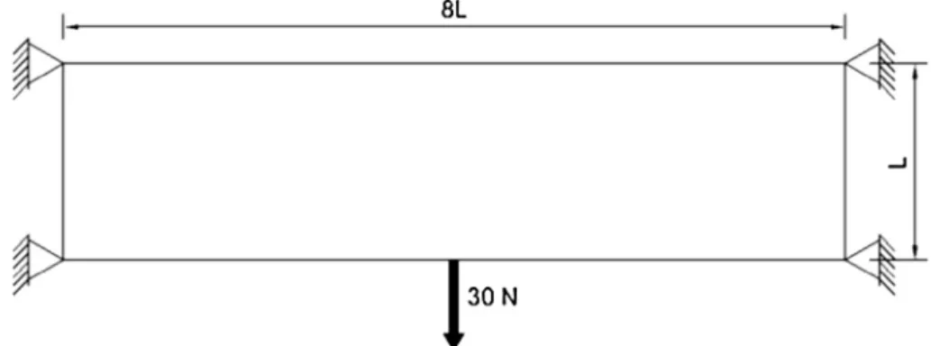
5.1. Plate attached at each end at the center node

This example consists of a rectangular plate simply supported at the center of both extremities. The load is applied upwards, in the upper center, and has the support conditions and structural geom-etry indicated inFig. 4.

The data for the problem has 2700 triangular finite elements in the linear analysis, and for the nonlinear analysis. The Young’s modulus is E= 10,000 N/cm2_{; the Poisson’s ratio is}

_t

_{= 0.3 and}

the thickness is 0.1 cm. For the linear analysis, the parameters are: final volume equal to 20%; the optimization procedure used

the parametersRR= 0.75%,ER= 1% and volume removal by itera-tion equal to 75%. For the nonlinear analysis, the same values apply, butRR= 3.5% andER= 5.85%.

These are the same data used by[5], for the same problem. The evolution of the optimization process during linear analysis is shown inFig. 5and is compared with the results obtained by[5], indicated inFig. 7. The evolution of the optimization process for the geometrically nonlinear analysis is shown in Fig. 6, which can be compared with that obtained by[5],Fig. 8.

By making a comparison between the maximum von Mises stress and the optimization iteration for linear and nonlinear cases, obtained was the graph indicated inFig. 9. Notice that the maxi-mum stress for the optimaxi-mum structure, when the nonlinear effect is considered, is around 1.2 times greater than the maximum ten-sion for the optimized linear configuration. Inevitably, the final

topologies are very distinct, since the influence of reaching the equilibrium condition in the deformed position creates stress flows that result in strong differences, showing how important it is to evaluate the optimization problem considering this effect in struc-tures where this phenomenon is relevant.

In addition, when a comparison is made between the displace-ments in accordance with each analysis, theFigs. 10 and 11are obtained, respectively.

Moreover, for the nonlinear analysis, it can be seen that the model presents a smooth curve, appearing in the interface between the linear and nonlinear results and remembering that the point of analysis is the same as that of the load application. Notice that for the final iterations, the geometrically nonlinear problem presents smaller displacements that the linear one. Furthermore, the slope

Fig. 4.Design domain of the supported plate.

Fig. 5.Optimal topology obtained by present model, linear analysis.

Fig. 6.Optimal topology obtained by present model, nonlinear analysis.

Fig. 7.Optimal setting by[5], linear analysis.

Fig. 8.Optimal setting by[5], nonlinear analysis.

Fig. 9.Maximum von Mises Stress versus number of iteration: both analyses of plate attached at each end at the center node.

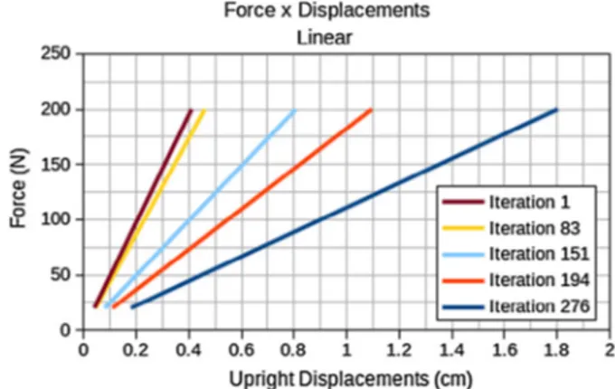
Fig. 10.Force versus Displacement during the iterative linear optimization process of plate attached at each end at the center node.

of the resulting curve for the nonlinear problem is greater than that of the linear case, consequently indicating greater structural stiffness.

5.2. A slender plate attached at the vertices

This example consists of a slender rectangular sheet simply supported at all vertices. The load is applied on the lower center, and has the support conditions and structural geometry displayed inFig. 12.

The data for the problem are: 2880 triangular finite elements in the linear analysis, and for the nonlinear analysis; the Young’s mod-ulus isE= 3000 N/cm2_{; the Poisson’s ratio is equal to 0.3, the}

thick-ness is 0.1 cm, the height is 2 cm and the length is 16 cm. For the linear analysis the parameters are: final volume equal to 40%, the optimization procedure used parametersER= 1.75%,RR= 1%, vol-ume removed per iteration is 1.75%. For the nonlinear analysis, the same values was applied, butRR= 3.5% andER= 10.75%.

This problem was also studied by[6]and by[17]. The optimal topology for linear analysis is indicated inFig. 13, and inFig. 14 is shown the optimal topology for the nonlinear analysis. The final optimum topologies found by[6]for the linear and nonlinear anal-ysis, respectively, are presented inFigs. 15 and 16.

When comparing the maximum von Mises stress of the itera-tions displayed inFig. 17, their behavior shows that the maximum stresses in the nonlinear cases are superior to those of the linear, as is expected.

Fig. 18displays a comparison between the displacements in accordance with each analysis. The displacements in the linear analysis increase a lot after the removal of the lower members, but beginning with a relatively smaller difference. Given their fast initial removal in the nonlinear analysis, the displacements already increase considerably in the third iteration, since the plate is long.

After this, the values undergo very small variation. In the present example, the curve is well defined, demonstrating the relevance of the nonlinearity for the model. For this same example, notice inFig. 19that the final iteration of the nonlinear problem displays an initial stiffness that is greater than in the linear case and increases in an asymptotic manner, characterizing an increase in structural stiffness for this type of analysis.

5.3. Square plate loaded at the geometric center

The design domain and the boundary conditions of the square plate are shown inFig. 20, designed to support a concentrated load of 20 kN.

The data for the problem are: 1800 finite elements for the linear analysis, and for the nonlinear analysis; the Young’s modulus is E= 2E6 N/cm2_{; the Poisson’s ratio is equal to 0.3, the thickness is}

1 cm. For the linear analysis the parameters are: final volume equal to 20%, the optimization procedure used parameters ER= 1.5%, RR= 1%, volume removal per iteration is 15%. For the nonlinear analysis, the same values apply, butRR= 3.5% andER= 12.75%.

This problem was also studied by[6]. The evolution of the opti-mization process for the linear analysis is shown inFigs. 21–23, the latter being its optimum topology.

The evolution of the optimization process for the geometrically nonlinear analysis using the formulation presented herein is shown inFigs. 24–26. The final optimum topologies found by[6] for the linear and nonlinear analyses are displayed in Figs. 27 and 28, respectively.

The optimized shape of this example is analogical with the opti-mized shape of the bi-supported square plate subject to pure

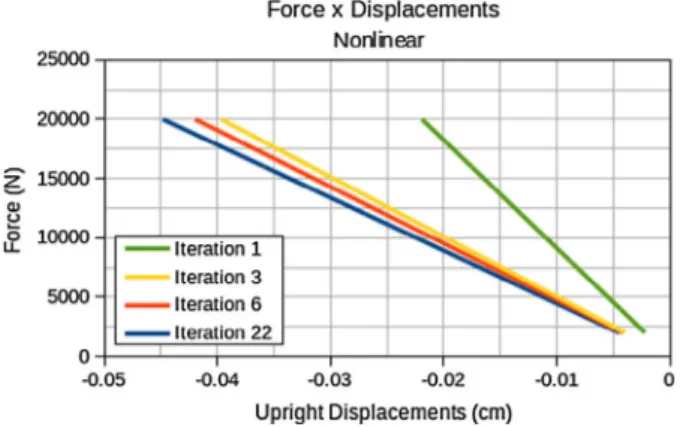
Fig. 11.Force versus Displacement during the iterative nonlinear optimization process of plate attached at each end at the center node.

Fig. 12.Design domain of the slender plate.

Fig. 13.Optimal topology obtained by present model, linear analysis.

Fig. 14.Optimal topology obtained by present model, nonlinear analysis.

shearing as presented in[17]. Notice that in the nonlinear case, the members subjected to compression result in a region of greater area in comparison with members subjected to tension, in contrast with the linear case, where they are almost symmetrical. This occurs in function of the nonlinear effect that mobilizes a greater compressed region, due to the second order effect that increases

the region of the compression struts.Fig. 29shows a comparison between the maximum stress for each iteration of the two models. It should be observed that the maximum stresses in the final topol-ogy for the linear case is 10% greater to that of the nonlinear one, since the compression struts in the linear model are narrower, gen-erating greater stresses. In the nonlinear case, greater stresses are found in the lower elements and for this reason, they are thicker compared to the linear ones.

Fig. 16.Optimal setting by[6], nonlinear analysis of a slender plate attached at the vertices.

Fig. 17.Maximum Von Mises Stress versus number of iteration: both analyses of a slender plate attached at the vertices.

Fig. 18.Force versus Displacement during the iterative linear optimization process of a slender plate attached at the vertices.

Fig. 19.Force versus Displacement during the iterative nonlinear optimization process of a slender plate attached at the vertices.

Fig. 20.Design domain of the square plate.

Fig. 21.Optimization history at iteration 30, linear analysis.

Fig. 30demonstrates a comparison between the displacements in accordance with each analysis. The displacement values from the linear analysis greatly increase during the last iterations, in contrast with those of the nonlinear analysis, where the values greatly increase in the first iterations (fast initial removal) and do

not undergo great alterations until the final optimum topology. The displacement values for final iterations of the nonlinear anal-ysis are less than those of the linear one, since the inclination of the straight line in the final iteration in the case of the nonlinear

Fig. 23.Optimal topology obtained by present model, linear analysis.

Fig. 24.Optimization history at iteration 3, nonlinear analysis.

Fig. 25.Optimization history at iteration 6, nonlinear analysis.

Fig. 26.Optimal topology obtained by present model, nonlinear analysis.

Fig. 27.Optimal setting by [6], linear analysis of square plate loaded at the geometric center.

Fig. 28.Optimal setting by[6], nonlinear analysis of square plate loaded at the geometric center.

Fig. 29.Maximum von Mises stress versus number of iterations: both analyses of square plate loaded at the geometric center.

one is greater than that of the linear one, i.e. the optimized form of the nonlinear problem presents greater stiffness than that of the linear problem. For this example, the curve of the linear analysis is smooth (short plate) since it is at the interface between the lin-ear and nonlinlin-ear ones, according toFigs. 30 and 31.

5.4. Support plate for an eolic turbine

The objective of this example is to apply the TO method pre-sented in this article for the optimization of a support plate to gen-erate electricity in an eolic turbine.

The optimized conception should present the same volume of the initial proposed conception, presented in[18], i.e., a new func-tional topology without holes.

The TO process begins with a rectangular plate base that is attached at each end on the left-hand side. A load distribution is applied on its upper side and has the dimensions displayed in Fig. 32. The objective of the analysis is to obtain the lightest

Fig. 31.Force versus Displacement during the iterative nonlinear optimization process of square plate loaded at the geometric center.

Fig. 32.Design domain of the suspended plate.

Fig. 33.Topology at iteration 10, linear analysis.

Fig. 34.Topology at iteration 28, linear analysis.

possible self-weight for the plate to meet the structural demands of supporting a turbine generator.

The data for the problem are: 2880 triangular finite elements for the linear and nonlinear analyses; the Young’s modulus is E= 2.05E7 N/cm2_{; the Poisson’s ratio is equal to 0.29, the thickness}

is 1 cm. For the linear analysis, the parameters are: the final vol-ume is equal to 45%, the optimization procedure used parameters ER= 2.5%,RR= 1.5%. For the nonlinear analysis, the same values apply, butRR= 3.5% andER= 4%.

The evolution of the optimization processes for the linear and nonlinear analyses are displayed inFigs. 33–38.

Fig. 39displays a comparison of the maximum stress of each iteration between the two models.

The results for the TO in geometrically linear and nonlinear con-ditions were similar due to the imposed initial concon-ditions (dis-tributed load) and the final volume to be achieved by the optimized structure. The achieved volume should be great so that the imposed load can be efficiently distributed to the turbine’s mast. It is notable that the topologies for both of the analyses

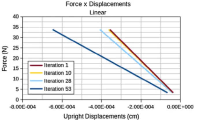
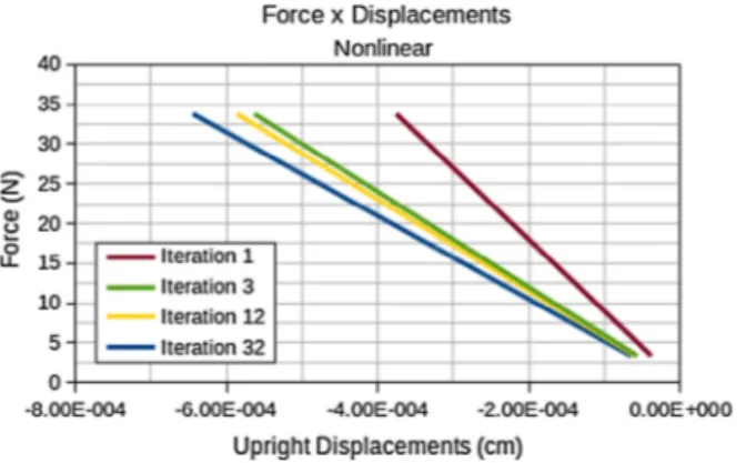
was similar, which suggests that the final optimum topology is ideal for the proposed problem. The maximum von Mises stress for both analyses were close to each other, seeFig. 37, guarantying that the optimization problem can be treated in a linear form when considering small displacements. The graphics inFig. 42present a comparison between the displacements in accordance with each analysis, as indicated inFigs. 40 and 41.

Fig. 36.Topology at iteration 3, nonlinear analysis.

Fig. 37.Topology at iteration 12, nonlinear analysis.

Fig. 38.Final optimum topology at iteration 32, nonlinear analysis.

Fig. 39.Maximum von Mises stress versus number of iterations: both analyses of support plate for a wind turbine.

The displacements, as well as the stresses of each analysis, were similar, reinforcing the hypothesis that the optimum topology is adequate for the considered problem.

6. Conclusion

The optimal topologies generated by the linear and nonlinear analysis, mainly when in presence of large displacements, can be completely different. Therefore, the geometric nonlinearities effects, in this case, are indispensable and must be incorporated into the topology optimization procedure in order to avoid yielding a false optimal topology or even an uneconomic structural design, if a linear analysis is carried out. The structures of the examples presenting with a moderate to large nonlinear geometric behavior, analyzed through curves load versus displacement during the iter-ative optimization process, show an optimal topology much stiffer than those linear ones. This demonstrates how important is to take into account these nonlinear geometric effects, mainly for those structures with large configuration changes. As already mentioned, the incorporation of these effects produce a different flux of stres-ses during the evolution of optimization and consequently in dif-ferent optimized shapes. In the last case presented, the linear and nonlinear geometric optimizations furnished almost the same solutions, but differed in the total number of iterations.

In all of the examples, significant differences were observed between the number of iterations needed to search for the linear and nonlinear geometric optimization solutions. Finally, different behaviors were observed for problems with concentrated and dis-tributed forces, suggesting that in the latter case, there was a smoothing of the initial conditions.

The main advantage of ESO based methods is that they do not require gradient calculation of the objective function, usually resulting in a faster convergence. Indeed, even the objective

function is not usually available for most of structural optimization problems found in real engineering applications[19]. The calcula-tion of the gradient is computacalcula-tionally expensive and for cases where the objective function presents discontinuity or complex functions this calculation is not always easy, or feasible, to achieve [20].

In conclusion, the SESO optimization method coupled with a positional finite element formulation applied for geometrically nonlinear plane stress problems proved to be precise and efficient, demonstrated by results that were very similar to those produced by other different methods and formulations.

Acknowledgements

The authors thank the brazilian sponsors: the Federal University of Minas Gerais (UFMG), the Federal University of Ouro Preto (UFOP), the Department of Structural and Foundation Engineering, School of Engineering of the University of São Paulo (EPUSP), the Brazilian Research Funding Agencies CAPES (Coordination of Improvement of Higher Education Personnel), CNPq (National Council of Scientific and Technological Development), and Minas Gerais State Research Foundation (FAPEMIG) for their financial supports, under Grant Numbers 304691/2009-7, 304275/2013-1 and TEC-PPM-00026-13.

References

[1]Vanderplaats GN. Numerical optimization techniques for engineering design: with applications. Boston: McGraw-Hill Book Company; 1984.

[2]Haftka RT, Gandhi RV. Structural shape optimization – a survey. Comput Meth Appl Mech Eng 1986;57:91–106.

[3]Bendsøe MP, Kikuchi N. Generating optimal topologies in structural design using a homogenization method. Comput Meth Appl Mech Eng 1988;71: 197–224.

[4] Sigmund O, Maute K. Topology optimization approaches – a comparative review. Struct Multidisc Optim 2013 [published online].

[5]Gea HC, Luo J. Topology optimization of structures with geometrical nonlinearities. Comput Struct 2001;79:1977–85.

[6] Chang DH, Yoo KS, Park JY, Han SY. Optimum design for nonlinear problems using modified ant colony optimization. In: International conference on software and computer application (ICSCA). Singapore; 2012.

[7]Almeida VS, Simonetti HL, Oliveira Neto L. Comparative analysis of strut-and-tie models using smooth evolutionary structural optimization. Eng Struct 2013;56:1665–75.

[8]Xie YM, Steven GP. A simple evolutionary procedure for structural optimization. Comput Struct 1993;49(5):885–96.

[9]Liang QQ, Xie YM, Steven GP. Topology optimization of strut-and-tie models in reinforced concrete structures using an evolutionary procedure. ACI Struct J 2000;97(2):322–30.

[10] Gea H, Luo J. Topology optimization of structures with geometrical nonlinearities. Comput Struct 2001;79:1977–85.

[11]Nishiwaki S, Frecker MI, Min S, Kikuchi N. Topology optimization of compliant mechanisms using the homogenization method. Int J Num Meth Eng 1998;42:535–59.

[12]Gea H, Jung HC. Topology optimization of nonlinear structures. Finite Elem Anal Des 2004;40:1417–27.

[13]Jansen M, Lombaert G, Schevenels M. Robust topology optimization of structures with imperfect geometry based on geometric nonlinear analysis. Comput Meth Appl Mech Eng 2015;285:452–67.

[14]Simonetti HL, Almeida VS, Oliveira Neto L. A smooth evolutionary structural optimization procedure applied to plane stress problem. Eng Struct 2014;75:248–58.

[15]Greco M, Ferreira IP. Logarithmic strain measure applied to the nonlinear positional formulation for space truss analysis. Finite Elem Anal Des 2009;45:632–9.

[16]Rades M. Finite element analysis. Romania: University Politehnica of Bucharest; 2006.

[17]Jung D, Gea C. Topology optimization of nonlinear structures. Finite Elem Anal Des 2004;40:1417–27.

[18]Lanes RM, Greco M. Application of a topological evolutionary optimization method developed through python script. Sci Eng J 2013;22:1–11 (in portuguese).

[19]Gournay F, Allaire G, Jouve F. Shape and topology optimization of the robust compliance via the level set method. ESAIM: Control, Opt Calc Variat 2008;14:43–70.

[20] Das R, Jones R, Xie YM. Optimal topology design of industrial structures using an evolutionary algorithm. Opt Eng 2011;12:681–717.

Fig. 41.Force versus Displacement during the iterative nonlinear optimization process of support plate for a wind turbine.

Fig. 42.Force versus Displacement of the final optimum topologies of each analysis.