Abstract
In the article, a new approach considering structural local failure for topology optimization of continuum structure is proposed. It aims at not only lowering the risk of local failure in the concerned structural regions, but also ensuring a good stiffness of the struc-ture. The local failure may be caused by the structural uncertain-ties or possible structural fatigue. To this end, a criterion to evalu-ate the effect of one local failure on the structure is introduced. This criterion is minimized to reduce the probability of structural damage based on an initialized structure whose compliance is opti-mized. Solid Isotropic with Material Penalization (SIMP) method and Optimality Criteria (OC) method are combined to solve the design problem. The effectiveness of the proposed algorithm is verified by a series of numerical examples. Furthermore, experi-ments merging with additive manufacturing technique are taken to prove the practical ability of the method in actual engineering.
Keywords
local failure, topology optimization, SIMP method, additive manu-facturing
Continuum Structural Layout in Consideration of the Balance
of the Safety and the Properties of Structures
1 INTRODUCTION
Since topology optimization emerged, it has been received increasing attention and has taken an important place in the activities of engineering design. There are thousands of research papers
pub-Hongxin Wang a Jie Liu a,b Xiuyang Qian a Xiaonan Fan a Guilin Wen a,*
a State Key Laboratory of Advanced
Design and Manufacturing for Vehicle Body, Hunan University, Changsha 410082, Peoples Republic of China
b Centre for Innovative Structures and
Materials, School of Civil, Environmental and Chemical Engineering, RMIT University, GPO Box 2476, Melbourne 3001, Australia
* Corresponding author: Tel.: +86 731 88823929; Fax: +86 731 88822051 Email: [email protected]
http://dx.doi.org/10.1590/1679-78253679
lished and also massive subjects about topology optimization to improve its application into engi-neering. Topology optimization is usually classified into two types, namely, topology optimization of discrete structures (Achtziger, 1997; Mortazavi and Toğan, 2016) and topology optimization of con-tinuum structures (Suzuki and Kikuchi, 1991; Sigmund, 2001; Wang et al., 2003; Bendsoe et al., 2013; Huang et al., 2010; Xie et al., 1993; Eschenauer et al., 1994; Aage et al., 2015). The former one’s target is to determine the optimum numbers, positions, and mutual connectivity of the struc-tural members. The latter one aims at finding the optimum distribution of material in a predefined design domain with given objectives and constraints (Frandsen et al., 2015; Dede et al., 2015; Jing et al., 2015; Fuchi et al., 2015; Christiansen et al., 2016; Otomori et al., 2016). Bendsøe and Kikuchi presented a method which makes the optimal shape design as the material distribution problem based on the theory of homogenization (Bendsøe and Kikuchi, 1988; Bendsøe, M. P. 1989). In addition, there is another research branch such as incorporating uncertainties into structural topology optimi-zation (Guest et al., 2008; Asadpoure et al., 2011; Chen et al., 2011; Liu et al., 2016; Jung et al., 2004; Schevenels et al., 2011; Liu et al., 2016; Xu et al., 2016; Xu et al., 2015). The method that we proposed in this article is to resist the structural local failure that may be caused by those uncer-tainties or possible structural fatigue.
With the risk of human’s errors and mistakes increasing, as well as the complexity of current structural mechanical properties, a limited redundancy and a good robustness for key structures is urgently needed. The collapse of the World Trade Centre towers and a number of collapses of struc-tural systems have demonstrated the importance of the strucstruc-tural fail-safe robustness (Sørensen et al., 2012). A structure with good fail-safe robustness can avert this situation, which can decrease the risk when a possible failure or crack emerges.
To our best knowledge, there are mainly two ways to consider the local failure in topology op-timization. One way is to set structural stress as constraints, to introduce the failure criterion (Ver-bart et al., 2013; Ver(Ver-bart et al., 2016), in which material is considered damaged when a stress con-straint is violated. The problem usually can be written as:
Minimize: Mass
Subject to: F(s( ) £x ) 0," Î Wx (1)
where the material failure function F depends on the stress field (x), and the constraint sets von
misses stress is usually seen as a yielding criterion of material for this kind of method. It is used to restrict the stress within a limit to eliminate the area of stress concentration and resist the occur-rence of damage. However, it is well-known that there are several difficulties to solve the concerned problems, such as singular optima, expensive computational cost and highly non-linear.
es-tablished a rigorous framework for fail-safe topology optimization of general 3D structures based on the method.
Analyzing the aforementioned remarkable works, most of them usually set the local failure as a constraint. They just attain the limit of the constraints for topology optimized designs but cannot minimize the effect of the worst damage case on the performance of the structures. In addition, some works remove the damaged regions with the form of patches to obtain the structure that is insensitive to the occurrence of a crack or a hole. However, many patches are removed in the final optimization results. Also, the aim of considering local failure in the optimization process should increase the safety under the premise of maintaining the properties of intact structures. But the aforementioned method just obtains a structure which is insensitive to the occurrence of a crack or a hole, not considering the stiffness of the intact structure. Therefore, a new approach is developed in this paper to balance the safety and the properties of structures. The method is to reduce the risk of prescribed regions which are to be possibly damaged in an initialized structure, at the same time, ensure the stiffness of the intact structure. To balance the safety and the stiffness, just a few areas are considered into the optimization objective, which are involved into one damaged scenario in the paper to reduce the computational cost. It should be pointed out that the possible damaged scenarios can be integrated by the Kreisselmeier-Steinhauser (KS) function (Jansen et al., 2014).A criterion which is also the optimization objective to evaluate the effect of one local failure on the initialized structure is introduced. The purpose of the method is to obtain the structure which gains the safety and a good stiffness at the same time.
This paper is organized as follows. Topology optimization method for continuum structures is briefly discussed in Section 2. The theory of damaged model in density-based topology optimization and the definition of influence coefficient of local failure on the optimized structure are respectively presented in Section 3. Section 4 presents an innovative algorithm considering local failure using the sensitivity analysis information. Section 5 shows some examples to demonstrate the effectiveness of the proposed algorithm. In section 6, the experiment merging with additive manufacturing is taken to affirm the practical ability of the method in actual engineering. Finally, the paper is closed with some concluding remarks.
2 TOPOLOGY OPTIMIZATION METHOD FOR CONTINUUM STRUCTURES
In this section, the general approach without considering local failure for topology optimization of continuum structure is overviewed briefly.
Topology optimization of continuum structure is to optimize the layout of material in the de-sign domain with prescribed boundary conditions and loadings. In the presented work, the SIMP method (Eschenauer et al., 1994; Bendsøe and Sigmund, 1999) is used. The design domain is discretized with finite elements, and the distribution of material is represented by a physical density
e
r per element, namely, the design variable which varies in the field of [0,1]. The Young’s modulus of element Ee is defined as follows:
e min
E = E +
0 min
( )
p
e E E
where E0 and Emin indicate the Young’s modulus of the solid and void of materials, respectively. p denotes penalization which is used to make intermediate densities inefficient in the optimization and tend to discrete 0-1 design. The elements’ Young’s modulus Ee is used to construct the global
stiffness matrix K in the finite element analysis:
0 p i i i r =
å
K k (3)( ) ( )r r =
K U F (4)
where 0 i
k denotes the elemental stiffness matrix associated with solid material properties. U is the
global displacement vector and F is the global load vector. In the traditional OC method, the compliance is usually set as the objective of optimization, and the problem after using the SIMP method can be formulated as follows:
0 1 Min N p T i i i i i
C r
=
=
å
u k u0
( ) subject to V f
V r £
KU =F
0<rmin £ £r 1
(5)
3 DAMAGE MODEL IN DENSITY-BASED TOPOLOGY OPTIMIZATION
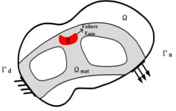
First, a mechanical body of an isotropic elastic material that occupies the design domain W ÎRd
(d=2 or 3) with a boundary that consists of two disjoint parts: G = G È Gd n is considered. A trac-tion force t is defined on
n
Figure 1: The damaged model in the design domain Ω, and the material domain Ωmat.
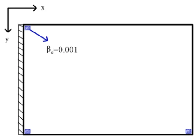
For damaged domain, in which the material is assumed degraded, accordingly, the Young’s modulus of material becomes Emin. To not affect the update of elemental densities in the process of
optimization, we introduce the coefficient be, where be =1 denotes material of the element
un-damaged, be =0.001 denotes material of the element damaged, by which every element will be endowed the coefficient like elemental density. The predefined damaged areas are described through endowing coefficient of the element with be =0.001, and the coefficient of other elements are
1 e
b = , then multiplying the coefficient by the elemental densities for all the elements. The func-tion of introducing the coefficient be is to hold the assumed areas of local failure in the final
struc-ture and do not affect the elemental density. A new global stiffness matrix K constructed with e b
is obtained as:
0
1 N
e e i i
b r
=
=
å
K k (6)
Then, the new equilibrium equation for damaged model becomes:
(b r, ) =
K W F (7)
where W denotes the global displacement of the damaged model, F is global load vector. The theory and equilibrium equation for the damaged model have been presented as above. Next, the criterion to evaluate the effect of one local failure on the structure will be discussed as follows.
3.1 The Influence Coefficient of Local Failure in Optimized Structure
Traditionally, compliance is the common optimization objective, which equals to the work of exter-nal load, expressed by the following formulation:
0
1 N
p T T
i i i i i
C r
=
where N denotes the number of elements, F and U are the global load vector and global dis-placement vector, respectively. Suppose that a crack or a hole occurs in the optimized structure, so materials in the region of crack or hole occurs become degenerated, resulting the coefficient of mate-rial turning from be( ) =i 1 to be( ) =i 0.001. The change leads to the change of the stiffness matrix
and W is obtained by E.q(7). The compliance of damaged model becomes:
T
C =F W (9)
where F is fixed. As mentioned in (Verbart et al., 2016), suppose that the overall performance of the structure can be measured by a scalar function that depends monotonically on the local materi-al properties. In that case, the damaged model will never perform better than the originmateri-al model. Therefore, in this purely mechanical problem, we use the compliance as a measure of the overall performance. Consequently, the damaged model will be always more (or at best equally) compliant:
T T
C =F W ³ C =F U (10)
The effect of local failure on the compliance of the structure can be weighed by the increased proportion between C and C, where the effect is the change of compliance between the damaged structure and original structure, indicating whether the structure is easy to be destroyed or not. An influence coefficient of local failure on the final design is introduced here in order to measure the aforementioned effect, where the percentage of the influence coefficient is adopted because the influ-ence coefficient for some smaller regions are too small and have trouble at sensitivity filtering. The coefficient is defined as:
C C C
G
C 100% (C 1) 100%
-= ´ = - ´ (11)
4 LOCAL FAILURE OF MATERIAL
In practice, it requires a good robustness for the optimized structure due to the uncertainties of manufacture and accidental event. Typically, modern structural design requires that consequence of damages to structures should not be fatal to the causes of damage.
Figure 2: The vertical displacements for intact model and damaged model.
(a) (b) (c) (d)
Compliance (N·mm) 220.5029 275.9644 275.9644 256.5163
Table 1: Compliance for intact model and damaged models.
The goal of the presented approach is to enhance the safety of structure based on the original structure. For balancing the safety and the properties better, usually, just some worst damaged scenarios are considered, the influence coefficient of these regions is set as optimization objective. Thus the design problem is formulated as follows:
Min:G (C 1) 100%
C
= - ´ (12a)
Subject to: 0 ( )
V f V
r
£ (12b)
:K( ) ( )rU r =F (12c)
:K(b r, )W( )r =F (12d)
:0<rmin £r£ 1 (12e)
where the second equilibrium equation in E.q(12d) is used to compute the displacement of the dam-aged model, the global stiffness matrix of the damdam-aged model is obtained based on the stiffness matrix of intact model in E.q(12c). The two equilibrium equations are performed simultaneously over all the iteration, so the computational cost is heavier, while the aim of involving the two equi-libriums is to obtain the designs which are insensitive to the occurrence of local failure at the prem-ise of guaranteeing the stiffness of the intact structure.
original structure. In the process of optimization, the structure derived in every iterative step will be assumed damaged in the predefined regions, however, the final optimization result holds the areas of predefined local failure.
4.1 Sensitivity Analysis
Based on the analysis mentioned above, the optimization objective considering local failure is shown in Equation (12a). Sensitivity analysis is needed when gradient-based optimization method is em-ployed to solve the above problem. Due to massive design variables, the adjoint method is adapted to obtain sensitivity analysis. The details of obtaining the total derivative of the objective function will be shown as follows. Using the chain rule, the total derivative of the objective function with regard to a design variable can be obtained as follow:
2 1
e e e
dG dC C dC
dr =C dr -C dr (13)
where C in the second term is the compliance of the original model, and it’s derivative can be de-rived by self-adjoint:
1 0
1 N
p T i i i i i
i
dC p
dr r
-=
= -
å
u k u (14)where ui denotes the nodal displacement vector per element, 0 i
k is the elemental stiffness matrix in
the original model. The derivative of the compliance of damaged model C in the first term of equa-tion (13) is also straightforward to derive. The coefficient of be is independent of density, so the
sensitivity also can be calculated using the self-adjoint.
1 0
1 N
p T i i i i i i
i
dC p
dr b r
-=
= -
å
w k w (15)where wi denotes the nodal displacement vector of the damaged model and ki0 is the elemental
stiffness matrix. Finally the sensitivity of the objective is shown as follow:
1 0 1 0
2
1 1
1 N p T N p T
i i i i i i i i i
i i
i
dG C
p p
dr C b r C r
-
-= =
= -
å
w k w -å
u k u (16)5 EXAMPLES
In this section, four numerical examples are discussed to illustrate the validity of the approach. Optimization results obtained by traditional approach and those obtained by the presented method are compared. In the examples, the neighborhoods of the loads and boundaries are also included to optimize, because the method just redistributes the elements based on the original structure. And the singularity for the computation of the point supports and point loads have been considered in the optimization. In the examples, just the regions which are easy to be damaged are only consid-ered.
5.1 Cantilever Beam
First, a simple example of optimizing cantilever beam is shown in Fig. 3 to test the proposed meth-od. The dimension of design domain is 100mm×60mm and is discretized by equally sized finite ele-ments with the size of 1mm×1mm. The volume fraction is limited to 0.5, the density is filtered using the filter radius R= 2. For the properties of the material, the Young’s modulus of solid mate-rial equals to E0 =1 Mpa, and the Poisson ratio is assumed 0.3. A unit external load F =1N is
imposed on the lower right corner.
Figure 3: Design domain and boundary conditions for cantilever beam.
Figure 4: The prescribed damaged regions which are in blue for cantilever beam.
(a) case 1 (b) case 2
(c) case 3 (d) case 4
Figure 5: Optimization results of the four cases for cantilever beam.
(a) (b)
(c)
Prescribed damaged regions {1≤x≤3,1≤y≤3} {1≤x≤3,57≤y≤59} {97≤x≤99,57≤y≤59}
Case 1 6.4894 3.3260 5.1119
Case 2 4.9662 3.2458 5.2692
Case 3 4.8789 2.7072 5.3080
Case 4 4.8892 2.7108 4.5046
Table 2: The influence coefficient in prescribed damaged regions for cantilever beam.
To observe the changes of influence coefficient in other regions, the distribution of densities for the optimized structure are recorded. The influence coefficient of each element calculated using Eq.(11) is shown in Fig. 7.
(a) case 1 (b) case 2
(c) case 3 (d) case 4
Figure 7: Diagrams of influence coefficient in the whole structure for cantilever beam.
increasing, influence coefficients of the element which are away from the optimized regions tend to increase accordingly. The goal of the method is to balance the safety and the stiffness, so the effect of other unimportant regions is not considered in the optimization. Although the influence coeffi-cients of some regions increase, the effect of local failure on the structure for these unimportant regions is little compared with the prescribed regions.
The selected regions (1,5) (1,10) (1,20) (1,30)
Case 1 0.6184 0.3940 0.2104 0.1025
Case 2 0.5041 0.3828 0.2504 0.1369
Case 3 0.4963 0.3852 0.2548 0.1442
Case 4 0.4960 0.3835 0.2579 0.1482
Table 3: Comparison of influence coefficient in some elements for cantilever beam.
5.2 MBB Beam
This example considers fail-safe robustness optimization in MBB beam. The boundary condition and dimension are shown in Fig. 8(a). The rectangular design domain is discretized into 130×40 mesh and the downward load is applied at the center of the top. The move limit becomes 0.1, the volume fraction is limited to 0.5, and other parameters are the same as the previous example. The prescribed damaged regions are plotted in Fig. 8(b). In the example, the size of assumed damaged regions is 10mm×3mm near the load and 5mm×5mm near the boundary. Where the coordinate coefficients are {60≤x≤70, 1≤y≤3}, {1≤x≤5, 36≤y≤40} and {126≤x≤130, 36≤y≤40} respectively, the elements on which the load and the boundary apply are excluded. And two cases are chosen, where case 1 is to optimize compliance, case 2 is to optimize the influence coefficient in these prescribed regions.
(a)
(b)
In Fig. 9, the optimization results of normal design and robust design are plotted respectively. It can be observed more obviously that the basic members don’t change, instead, angles and posi-tions change a lot. From the structural point of view, the approach is to optimize the layout of members to change the load path and strengthen the prescribed regions. The final compliance for intact model and damaged model obtained by traditional method and presented method are listed in Fig. 10, which illustrate the superiority of the method at balancing the safety and the stiffness of structures. The influence coefficients of each area with the size of 2mm×2mm in the whole design domain are calculated using Eq. (11), and are shown in Fig. 11. The elements which are applied load and boundary constraints are excluded to avoid the singularity for calculating the influence coefficient. Then the max influence coefficient in each prescribed damaged region is listed in Table 4.
(a) case 1
(b) case 2
Figure 9: The optimization results of the two cases for MBB beam.
(a) case 1 (b) case 2
Figure 11: Diagrams of influence coefficient in the whole structure for MBB beam.
Prescribed damaged regions
1 2
37 38
x y £ £ £ £
61 62
1 2
x y £ £
£ £
129 130
37 38
x y £ £ £ £
Case 1 13.3386 2.8749 13.3386
Case 2 12.7611 2.8683 12.7611
Table 4: The maximal influence coefficient in prescribed damaged regions for MBB beam.
5.3 L-Bracket
Then the effectiveness of the method will be tested in L-type beam. The structure is modeled using four node finite elements with the size of 1mm×1mm, where the number of elements is 6400. The volume constraint is 30% of the design domain; other parameters are identical to those used in ex-ample 5.1. The external load is F =1N and is imposed on the top of the lower right corner (shown
in Fig. 12).
In the example, two cases are compared. The first case is to optimize compliance which is called L1, the second is to optimize the influence coefficient in the region of {36≤x≤45, 56≤y≤65} (Fig. 13) which is easy to be damaged and is called case L2. It is supposed that the size of local failure is 10mm×10mm, because the corner in the L bracket is very important, so the predefined region is larger than other examples. And the optimization results of normal design and robust design are shown in Fig. 14.
Figure 13: The prescribed damaged region which is in blue for L-bracket.
(a) case L1 (b) case L2
Figure 14: Optimization results of the two cases for L-bracket.
members alter the load path, which offer more braces for the corner. Also the compliance of intact model and the damaged model for case L1 and case L2 are compared in Fig. 15, which justifies that the method is to improve the stiffness of damaged model at the premise of keeping the good proper-ties of intact model. Also the objective function of G decreases greatly, which indicates that the method is valid. Then the elemental densities for the optimized structure are used to calculate the influence coefficients of each element, and they are shown in Fig. 16. The maximal influence coeffi-cient near the structural corner is selected from the diagram and is listed in Table 5.
Figure 15: The comparison of compliance of intact model and damaged model for L bracket.
(a) case L1 (b) case L2
Figure 16: The influence coefficient of each element in the L-bracket for the two cases.
Some selected regions (41,61) (1,1) (40,1)
Case L1 1.9723 0.3082 0.2689
Case L2 0.7330 0.2803 0.2767
Table 5: Comparison of influence coefficient in some local regions for L-bracket.
5.4 U-Shape Structure
In the last test, the U-shape structure is optimized to verify the proposed algorithm. The design domain has a width of 120mm and a length of 100 mm, the mesh size of each element is defined as 1mm×1mm, so the total elements number of design domain is 10400. The external load and bound-ary condition are shown in Fig. 17(a). The volume constraint is 30% of the design domain. In Fig. 17(b), the prescribed damaged regions are shown in blue. And two cases are compared, where case 1 is to optimize compliance and case 2 is to optimize the scenario that assume local failures occur in the prescribed regions.
(a)
(b)
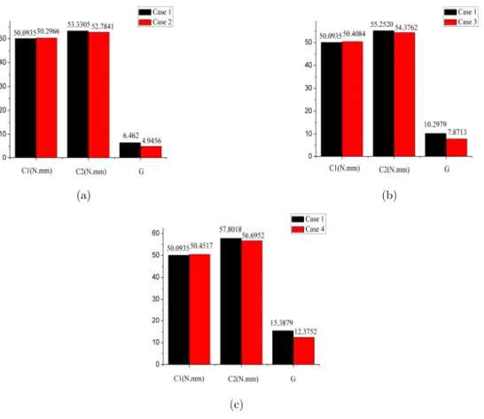
The compared results are shown in Fig. 18(a) and (b) respectively. It can be obviously seen that the predefined regions are strengthen by more elements compared with the normal design. Also, new bars appear to resist the damage, and the critical section in case 2 is stronger than case 1, which, once again, illustrate that the algorithm is to redistribute the elements or members based on the normal structure. For the U-shape structure, it is obvious that the two corners are the most serious areas where the stress concentrates, so they are the only prescribed optimization regions when the components are used under the regular work. The compliance of intact model and dam-aged model are also compared, which is more intuitive to illustrate the availability of the method. In Fig. 19, C1 is the compliance of intact model, C2 is the compliance of damaged model and the G is the optimization objective. The influence coefficient of each element is shown in Fig. 20, where the influence coefficients in the prescribed regions are listed in Table 6. From the Table 6, it can be seen that the reduced proportion of influence coefficient approaches to 50%, which demonstrates the effectiveness of the method once again.
(a) case 1 (b) case 2
Figure 18: The optimization results of the two cases for U-shape structure.
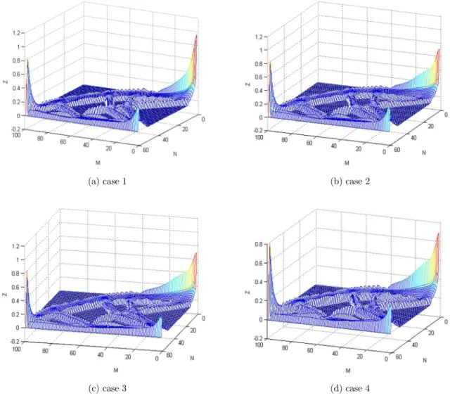
(a) case 1 (b) case 2
Figure 20: The influence coefficient of each element in the U-shape structure for the two cases.
The prescribed regions (80,31) (80,70)
Case 1 2.0896 2.0896
Case 2 1.1230 1.1230
Table 6: Comparison of influence coefficient in prescribed regions for U-shape structure.
6 THE EXPERIMENT COMPARISON BY ADDITIVE MANUFACTURING
In this section, the effectiveness of the method will be proved further through the test with the op-timization results listed in the last section, and the optimal structures are fabricated by additive manufacturing. Due to the limit of experimental equipment, only the MBB beam and the U-shape structure are selected in the test. The experiment simulates the loading and boundary condition on the tensile machine, and tests the additively manufactured components to verify the effectiveness of the method in the practical engineering. The details are stated as follows.
6.1 Additive Manufacturing Related to Topology Optimization
Additive manufacturing, which is known as 3D printing is popular recently because of the superiori-ty at the fabrication of the components with the geometrical complexisuperiori-ty. Topology optimization, which is restricted at the conceptual design due to traditional manufacturing process is hard to fabricate the complex structure created by topology optimization, such as casting and machining. However, the advanced development of the additive manufacturing makes them an ideal fit.
Much less re-engineering needed; (3) Optimal performance remains intact. Therefore, it will be a promising research direction for the topology optimization with additive manufacturing.
6.2 The Experiment of MBB Beam
First, the optimization results of MBB beam shown in the section 5.2 were built artificially in the SolidWorks. Unavoidably, there would be some deviations with theoretical results due to the inter-mediate densities near the boundary. However, we had tried our best to draw it as a unified stand-ard to decrease the effect. For increasing the accuracy, we endued the plane optimization results a thickness of 10mm. Then the test specimens were additively manufactured by means of the fused filament fabrication technique (Clausen et al., 2016) using a machine of Makerthink x1, where the printing material adopts polylactide (PLA). The aim of the experiment is to compare the structures obtained with the two different algorithms, so the influence of the material and the influence of infill density can be ignored. The fill density is 20% of the whole structure, and the filament was extruded with a layer height of 0.2 mm and an extrusion width of approximately 0.4 mm.
With the components fabricated by additive manufacturing, the three-point bending test of MBB beam was carried on the tensile machine of TFW-108. A steel loading head was placed on the loading point of the beam, and the beam was placed on the two supports of the steel bracket (shown in Fig. 21) to simulate the loading and boundary condition in the problem of topology op-timization. The loading head was applied on the loading point with the velocity of 5mm/min, the data of force and displacement was measured by the transducer in the machine and was plotted as curve. The components of normal design and robust design fabricated by additive manufacturing were tested uniformly as the step. Where the test results are shown in Fig. 22, and the curves of force and displacement are shown in Fig. 23. Seen from the test results, the component of case 1 lost the ability of normal working because of the entire fracture at one side of the supports, due to some uncertainties of manual operations, there may be some mistakes that cause the case 1 which is symmetric just fractured at one side. For case 2, the component were injured at the two supports, however, it still survived for a long time, which can be observed clearly from the curve of force and displacement. And seen from the curve, the displacement of case 2 is larger than the displacement of case 1 when the structure is damaged. In other words, the structure of case 1 is destroyed howev-er the structure of case 2 is safe when these two structures undhowev-ergo the identical strain.
(a) case 1 (b) case 2
Figure 22: The experiment results of the two cases for MBB beam.
Figure 23: The force-displacement curve of the two cases for MBB beam.
6.3 The Experiment of U-Shape Structure
Figure 24: The loading condition on the tensile machine for U-shape structure.
Figure 25: The curve of force and displacement for aramid fiber.
(a) case 1 (b) case 2
Figure 26: The experiment results for U-shape structure.
Figure 27: The curve of force and displacement for U-shape structure.
7 CONCLUSIONS
introducing a constraint of length scale control on the member to ensure the safety of some thin members in the final results.
Acknowledgment
The second author is partially supported by the scholarship No. 201506130053 of China Scholarship Council. This work was supported jointly by the project of “Chair Professor of Lotus Scholars Pro-gram” in Hunan province, the National Natural Science Foundation of China (No. 11672104 and No.11302033) and the National Science Fund for Distinguished Young Scholars in China (No. 11225212). The authors also would like to thank the support from the Collaborative Innovation Center of Intelligent New Energy Vehicle, and the Hunan Collaborative Innovation Center for Green Car.
References
Aage, N., Andreassen, E., & Lazarov, B. S. (2015). Topology optimization using PETSc: An easy-to-use, fully paral-lel, open source topology optimization framework. Structural and Multidisciplinary Optimization, 51(3), 565-572. Achtziger, W. (1997). Topology optimization of discrete structures. In Topology optimization in structural mechanics (pp. 57-100). Springer Vienna.
Asadpoure, A., Tootkaboni, M., & Guest, J. K. (2011). Robust topology optimization of structures with uncertainties in stiffness–Application to truss structures. Computers & Structures, 89(11), 1131-1141.
Bendsøe, M. P. (1989). Optimal shape design as a material distribution problem. Structural optimization, 1(4), 193-202.
Bendsøe, M. P., & Kikuchi, N. (1988). Generating optimal topologies in structural design using a homogenization method. Computer methods in applied mechanics and engineering, 71(2), 197-224.
Bendsøe, M. P., & Sigmund, O. (1999). Material interpolation schemes in topology optimization. Archive of Applied Mechanics, 69(9-10), 635-654.
Bendsøe, M. P., & Sigmund, O. (2013). Topology optimization: theory, methods, and applications. Springer Science & Business Media.
Ben-Tal, A., & Nemirovski, A. (2002). Robust optimization–methodology and applications. Mathematical Program-ming, 92(3), 453-480.
Bourell, D. L. (2016). Perspectives on Additive Manufacturing. Annual Review of Materials Research, 46, 1-18. Chen, S., & Chen, W. (2011). A new level-set based approach to shape and topology optimization under geometric uncertainty. Structural and Multidisciplinary Optimization, 44(1), 1-18.
Christiansen, R. E., & Sigmund, O. (2016). Designing meta material slabs exhibiting negative refraction using topol-ogy optimization. Structural and Multidisciplinary Optimization, 1-14.
Clausen, A., Aage, N., & Sigmund, O. (2016). Exploiting Additive Manufacturing Infill in Topology Optimization for Improved Buckling Load.Engineering, 2(2), 250-257.
Dede, E. M., Joshi, S. N., & Zhou, F. (2015). Topology optimization, additive layer manufacturing, and experimental testing of an air-cooled heat sink. Journal of Mechanical Design, 137(11), 111403.
Eschenauer, H. A., Kobelev, V. V., & Schumacher, A. (1994). Bubble method for topology and shape optimization of structures. Structural optimization, 8(1), 42-51.
Frangopol, D. M., & Curley, J. P. (1987). Effects of damage and redundancy on structural reliability. Journal of Structural Engineering, 113(7), 1533-1549.
Fuchi, K., Ware, T. H., Buskohl, P. R., Reich, G. W., Vaia, R. A., White, T. J., & Joo, J. J. (2015). Topology opti-mization for the design of folding liquid crystal elastomer actuators. Soft Matter, 11(37), 7288-7295.
Guest, J. K., & Igusa, T. (2008). Structural optimization under uncertain loads and nodal locations. Computer Methods in Applied Mechanics and Engineering, 198(1), 116-124.
Huang, X., & Xie, M. (2010). Evolutionary topology optimization of continuum structures: methods and applications. John Wiley & Sons.
Jansen, M., Lombaert, G., Schevenels, M., & Sigmund, O. (2014). Topology optimization of fail-safe structures using a simplified local damage model. Structural and Multidisciplinary Optimization, 49(4), 657-666.
Jing, G., Isakari, H., Matsumoto, T., Yamada, T., & Takahashi, T. (2015). Level set-based topology optimization for 2D heat conduction problems using BEM with objective function defined on design-dependent boundary with heat transfer boundary condition. Engineering Analysis with Boundary Elements, 61, 61-70.
Jung, H. S., & Cho, S. (2004). Reliability-based topology optimization of geometrically nonlinear structures with loading and material uncertainties. Finite Elements in Analysis and Design, 41(3), 311-331.
Liu, J., Wen, G., & Xie, Y. M. (2016). Layout optimization of continuum structures considering the probabilistic and fuzzy directional uncertainty of applied loads based on the cloud model. Structural and Multidisciplinary Optimiza-tion, 53(1), 81-100.
Liu, J., Wen, G., Zuo, H. Z., & Qing, Q. (2016). A simple reliability-based topology optimization approach for con-tinuum structures using a topology description function. Engineering Optimization, 48(7), 1182-1201.
Mortazavi, A., & Toğan, V. (2016). Simultaneous size, shape, and topology optimization of truss structures using integrated particle swarm optimizer. Structural and Multidisciplinary Optimization, 1-22.
Otomori, M., Yamada, T., Izui, K., Nishiwaki, S., & Andkjær, J. (2016). Topology optimization of hyperbolic met-amaterials for an optical hyperlens. Structural and Multidisciplinary Optimization, 1-11.
Schevenels, M., Lazarov, B. S., & Sigmund, O. (2011). Robust topology optimization accounting for spatially varying manufacturing errors. Computer Methods in Applied Mechanics and Engineering, 200(49), 3613-3627.
Sigmund, O. (2001). A 99 line topology optimization code written in Matlab. Structural and Multidisciplinary Opti-mization, 21(2), 120-127.
Sørensen, J. D., Rizzuto, E., Narasimhan, H., & Faber, M. H. (2012). Robustness: theoretical framework. Structural Engineering International, 22(1), 66-72.
Suzuki, K., & Kikuchi, N. (1991). A homogenization method for shape and topology optimization. Computer Meth-ods in Applied Mechanics and Engineering, 93(3), 291-318.
Verbart, A., Langelaar, M., & van Keulen, F. (2013). A new approach for stress-based topology optimization: Inter-nal stress peInter-nalization. In Proceedings of the 10th World Congress on Structural and Multidisciplinary Optimization. USA, Orlando.
Verbart, A., Langelaar, M., & van Keulen, F. (2016). Damage approach: A new method for topology optimization with local stress constraints. Structural and Multidisciplinary Optimization, 53(5), 1081-1098.
Verbart, A., Langelaar, M., & van Keulen, F. (2016). Damage approach: A new method for topology optimization with local stress constraints. Structural and Multidisciplinary Optimization, 53(5), 1081-1098.
Wang, M. Y., Wang, X., & Guo, D. (2003). A level set method for structural topology optimization. Computer Methods in Applied Mechanics and Engineering, 192(1), 227-246.
Xie, Y. M., & Steven, G. P. (1993). A simple evolutionary procedure for structural optimization. Computers & Structures, 49(5), 885-896.
Xu, B., Zhao, L., Xie, Y. M., & Jiang, J. (2015). Topology optimization of continuum structures with uncertain-but-bounded parameters for maximum non-probabilistic reliability of frequency requirement. Journal of Vibration and Control, 1077546315618279.