Implementing a computer algebra system in Haskell
Jose´ Romildo Malaquias
a, Carlos Roberto Lopes
b,*aDepartamento de Computac¸a˜o, Universidade Federal de Ouro Preto, Ouro Preto, Brazil bFaculdade de Computac¸a˜o, Universidade Federal de Uberlaˆndia, Uberlaˆndia, Brazil
Abstract
There are basically two kinds of mathematical computation, numerical and symbolic. Numerical algorithms are usually implemented in strongly typed languages, and compiled with a view to efficiency. Symbolic algorithms are mostly written for interpreters in untyped languages. Therefore, symbolic mathematics is usually slow, and bug ridden. Since symbolic algorithms are usually more difficult to implement, there are also very few computer algebra systems. This paper presents a computer algebra system that is both fast, and implemented in a strongly typed language, and designed to accept com-piled extensions. The authors describe a scheme to achieve these goals without creating difficulties for the end-user. The reason for creating this new computer algebra system is to make feasible mixed computation, i.e., programming software that needs both numerical computation and computer algebra. For instance, Finite Element Methods require a lot of num-ber crunching as well as computer algebra to perform triangularization, manipulating shape functions, etc. Mixed compu-tation requires speed and safety that interpreted computer algebra cannot provide.
2007 Elsevier Inc. All rights reserved.
Keywords: Computer algebra; Mixed computation; Functional programming; Haskell
1. Introduction
Computers have been used for numerical computations since their beginning. These general purpose machines can also be used for transforming and combining symbolic expressions as well. That is, computers can be used not only to deal with numbers, but also with abstract symbols representing mathematical formu-las. This fact was realized much later and is only now gaining acceptance among mathematicians and engineers.
According to Winkler [1] in his short introduction to Computer Algebra, before 1850 mathematicians solved the majority of their problems by extensive calculations. However in the 19th century, the style of mathematical research changed from quantitative to qualitative aspects. The advent of modern digital com-puters and the development of Computer Algebra programs in the 20th century stressed this trend. Notwith-standing even today many mathematicians think that the role of computers is number crunching and their role
0096-3003/$ - see front matter 2007 Elsevier Inc. All rights reserved.
doi:10.1016/j.amc.2007.02.126 * Corresponding author.
E-mail address:[email protected](C.R. Lopes).
is the application of the appropriate algebraic transformations to the problem and thus underestimating the power of computing systems for algebraic manipulation, which was recognized as early as 1844 by Lady Augusta Ada Byron, countess of Lovelace. In describing the possible applications of the Analytical Engine
developed by Charles Babbage, she wrote[1]:
‘‘Many people who are not conversant with mathematical studies imagine that because the business of [Babbage’s Analytical Engine] is to give its results in numerical notation, the nature of its process must consequently be arithmetical and numerical rather than algebraic and analytical. This is an error. The engine can arrange and combine its numerical quantities exactly as if they were letters or any other gen-eral symbols; and in fact it might bring out its results in algebraic notation were provisions made accordingly.’’
Indeed a modern computer is a universal machine that is able to carry out an arbitrary algorithm, being it numerical, symbolic or of any other nature.
What does one mean by Computer Algebra or symbolic algebra computation? R. Loos wrote[2]:
‘‘Computer Algebra is that part of computer science which designs, analyzes, implements, and applies algebraic algorithms.’’
Algebraic algorithms are algorithms that utilize the rules of Algebra to transform algebraic formulas con-taining numbers, variables and function applications. In short, Computer Algebra systems deal not only with integers and reals, but also with variables representing unknown quantities and any expression combining numbers and variables by means of mathematical operations. Numbers are represented exactly. The approx-imations of floating point numbers for reals are not acceptable anymore. So there is no need to be concerned about approximation errors.
Computer Algebra software finds application in any field dealing with the formulation oflawsin mathemat-ical terms, using algebraic equations and/or analytic concepts such as ordinary, partial differential equations and integrals. After the formulation of a law, it should be solved, simplified or reduced to the normal form. This process can be performed with help of Computer Algebra. Normal form is a concept that changes from one branch of Mathematics to another. For instance, in Lambda Calculus, a term in the normal form has no subterms of the formðkx:R SÞ, i.e., terms that can be lambda reduced. In relational algebra, one may have another definition. The fact is that the existence of the normal form makes it possible to compare expressions. After a sequence of transformation, one expects that two equivalent expressions be reduced to the same nor-mal form. In this work, the reader will find a definition of nornor-mal form that allows one to compare two seman-tically equivalent algebraic expressions.
Nowadays there are a handful of programs which perform Computer Algebra. These programs can be applied in areas such as Mathematics, Computer Science, Engineering, Economics, etc. With these pro-grams one can perform algebraic simplifications as well as handle literals, as illustrated by the following examples.
5a
22abþb2
ab ¼5aþ5b;
d dxðax
2þbxþcÞ ¼2axþb;
sin2aþcos2
a¼1:
Most of these programs suffer drawbacks. For instance, their programming languages are not referentially transparent, that is, they do not allow substitution of equals for equals, invalidating the use of certain Math-ematical laws. Even if other areas of thought are able to do without substitution of equals for equals, this is not true of Mathematics, the main subject of Computer Algebra. Therefore, the absence of referential trans-parency is a mortal sin, when it occurs in a Computer Algebra language.
The notion of transparency is due to Whitehead and Russell[3]. Antoni Diller[4]illustrates the invalidation of substitution in natural languages with the following sentence drawn from Russell[5]:
It should be noted that the above sentence is true, since the mad king really wished to know whether Scott was the author of Waverley. However, we do know that Scott and the author of Waverley are indeed the same person. Therefore, we may feel entitled to substitute Scottforthe author of Waverley in Russell’s sentence. In doing so, we get
George IV wished to know whether Scott was Scott.
The result is obviously false, for even being mad, the King knew well that Scott was Scott.
Imperative computer languages suffer from the same lack of transparency as natural languages. For exam-ple, one cannot make use of the commutative property of multiplication to conclude that the C program of listing 1 will print the same number twice, althoughfð2Þ gð5Þ ¼gð5Þ fð2Þin Mathematics. This happens because C functions may change the state of the computing system (by means of assignments to variables) besides (possibly) computing a value. In listing 1 functiong changes the contents of the global variable k
before returning a value and functionfneeds the value ofkin order to compute its result. So calls toghave an effect on calls tof. The return value offdepends on the previous calls tog. This program outputs6¼99 and shows that C is a referentially opaque language. Thus it is highly desirable that the language used to express Computer Algebra algorithms be referentially transparent.
This work has three phases. The authors started by implementing a computer algebra system in Scheme, an imperative language of the LISP family. This was done so as to become familiar with computer algebra algo-rithms by performing a traditional implementation. Besides this, a working Scheme system could be used for comparison, and prototyping. The next step was to implement a Computer Algebra library for Haskell, a lan-guage with the desired referential transparency property, highly popular, and quite flexible, which facilitates the creation of novel algorithms. The Haskell implementation was used as a proof of concept. The next and last step was to translate the Haskell implementation to Clean, a highly efficient language of the same family as Haskell. Then the main purpose of this work is to provide algorithms for manipulation of algebraic expres-sions in a declarative context, compatible with Mathematics, and implement them as a language for Computer Algebra programming embedded in Clean. Its implementation is one more example that shows that functional languages are viable for day to day programming, even beating conventional languages in some aspects, such as the level of abstraction, and even in speed, when the algorithms involve memory manipulation and data structures.
10 years to check it (vide[6]). One hundred years after Delaunay’s efforts Henrard and Rom[7]used a rather primitive computer algebra program to check Delaunay’s work. According to Henrard in a private commu-nication to us, their Computer Algebra program was able to get the result in less than 24 h. The program was almost 1000 times faster than Delaunay. The conclusion is that for purely algebraic problems the speed of available Computer Algebra systems is more than enough. However, numerical calculations often have a strong symbolic component. For instance, the Finite Element Method requires handling shape functions, per-forming triangularization, and finding a node renumbering schemes that produce narrow band matrices. Since these tasks may be performed concurrently with numerical calculations, an efficient Computer Algebra system may be useful.
The development of this library has also lead us to identify some limitations of Haskell and Clean, as well as extensions to these languages that would make the implementation easier and more elegant. These limitations are described in the paper through examples drawn from the library.
The rest of this paper is organized as follows. Section2 presents related works in the area, describing the most popular Computer Algebra Systems. Section3provides a short overview of functional programming lan-guages, which are derived from the Lambda Calculus. Section4describes some relevant aspects of the system design and implementation. Section5discusses some limitations in Haskell that make the library more difficult to design and implement. Finally, Section 6concludes the discussion.
2. Related work
According to Nilsson[8], research in Computer Algebra had its beginnings when James Slagle created the program Saint, which was able to integrate functions by elementary methods. After this first step, Joel Moses improved the algorithms of Saint, creating another program of symbolic integration, which was named SIN. In the sixties, Carl Engleman, Joel Moses and William Martin (at the Massachusetts Institute of Technol-ogy, as part of the MAC project) started the projectMacsyma1[9], which is one of the finest systems of Sym-bolic Mathematics. It is quite large, and written in Lisp. After Macsyma, many other systems of Computer Algebra came to light. Each one of these systems tried to correct a real or imaginary weakness of Maclisp, the original computer language of Macsyma. Some of these systems are:
• Reduce.2In the beginning, Lisp had many dialects. In general, every machine had its own dialect. Macsyma
was developed in Maclisp. Therefore, one could not build the system in a machine running Franz Lisp, Interlisp, etc. The designers of Reduce[10,11]proposed a standard dialect of Lisp, which should be porta-ble to any machine. Although Reduce became very popular, Standard Lisp was badly beaten by Common Lisp in the struggle to become the standard dialect of the main AI language. In the meantime, Macsyma migrated from MACLISP to Common Lisp. The result is that Macsyma runs in a standard language, while Reduce is built on top of an obscure dialect known as Standard Lisp.
• Maple.3Lisp always had a bad reputation for being slow. Therefore, Maple[12]was developed (at
Water-loo University, Canada) in a procedural language (C) with a view to greater efficiency. Since procedural languages like C are not fit for symbolic computation, the implementors of Maple were forced to design a symbolic language. Not being experts in compiler construction, they wrote an interpreter for the Maple language. The result is that Maple is much slower than Macsyma and other Lisp based systems. Maple’s source code is not in the public domain.
• Derive.4This package (and its precursorMuMATH) was designed to offer a small and fast Computer
Alge-bra system[13]. It was the only competitor to Macsyma that really delivered on its promises. The system is indeed very small and reasonably fast. However, it did not meet the commercial success of Reduce and Maple.
1 http://www.macsyma.com/
2 http://www.rrz.uni-koeln.de/REDUCE 3 http://www.maplesoft.com/
Maple, Reduce and Derive were designed to be worthy competitors of Macsyma. There are also systems designed to offer limited functionality in a friendly environment. Among these systems, MatLab5 [14] and
Mathematica6[15]became very popular. It is interesting to note that these two systems that promised limited functionality also failed to deliver on their promise. Due to demands from the market, the implementors of both Matlab and Mathematica have increased the functionality of their systems, which soon became as fat as Reduce. However, neither Matlab nor Mathematica have the well designed architecture of Reduce. In fact, these systems suffered from a chaotic growth.
3. A short overview of functional programming
In this section we describe the main concepts related to functional programming. Functional programming has roots in the lambda calculus. We start by describing the syntax and semantics of the lambda calculus. After we show that lambda calculus presents all the features existent in modern functional programming lan-guages such as Haskell and Clean. In reality a pure functional programming language is an applied lambda calculus.
3.1. Lambda calculus
Functional programming has roots in the lambda calculus. The lambda calculus is a branch of logic, devel-oped in the 1920s and 1930s by logicians who wanted to explore how to define functions formally and how to use this formalism as a foundation for mathematics. The lambda calculus is a simple and powerful formal lan-guage of functions. The first developments were made by Scho¨nfinkel[16], and Curry[17]who defined a var-iation called combinatory logic. Later, Church [18] defined the first version of the actual lambda calculus. Note that these early logicians had no intention of defining any programming languages. Actually, there wer-en’t even any computers at that time. The syntax of the lambda calculus is very simple, because there are only three types of constructs: variables, abstractions, and applications. A brief notion of the meaning of each one of the constructs (intuitive semantics) follows:
1. The variables are just place holders for values. In this section we use lowercase letters for representing vari-ables such asx;y;f;g.
2. Abstraction is a model for function definition, which is not associated to any name. In terms of syntax an expressionkx:Mdenotes an abstraction. The variablexis the parameter of the function, and the expression
Mis the body of the function. All occurrences ofxinkx:M are said to bebound. All unbound occurrences of a variable in a term arefree.
3. Applications are a model for the computation of a functional value. In a lambda expression like (M1M2), the first item (called therator, from operator) is applied to the second item (called therandfrom operand).
In a lambda term like (M1M2), ifM1 (sometimes called theapplicand) is an abstraction, the term may be reduced.M2, the argument, may be substituted into the body ofM1in place of the formal parameter ofM1
and the result is a new lambda term which is equivalent to the old one. As we mentioned earlier, if a lambda term contains no subterms of the formðkx:M1 M2Þthen it cannot be reduced, and is said to be in a normal form. The expressionfN=xgM represents the result of taking the termMand replacing all free occurrences of
xwithN. Thus we write
ðkx:M NÞ ! fN=xgM
The right sidefN=xgM is considered to be simpler thanðkx:M NÞ. This reduction is known asb-reduction. There is an additional rule calleda-conversion, which renames bound variables:
kx:M !ky:fy=xgM y not free inM
Ab-reduction reduction captures the essential behavior of all mathematical functions. For instance, consider the function that computes the square of a number. We might write
The square of xisxx
In the specification above we use the symbol ‘*’ to indicate multiplication. The symbolxis the formal param-eter of the function. To evaluate the square for a particular argument, say 2, we insert it into the definition in place of the formal parameter:
The square of 2 is 22
In order to evaluate the resulting expression 2 * 2 it is necessary to know what the number 2 means and how to multiply two numbers. Since any computation is simply a composition of the evaluation of suitable functions on suitable primitive arguments, this simple substitution principle suffices to capture the essential mechanism of computation.
With respect to the previous example it is important to notice that the number 2 and multiplication oper-ator ‘*’ belong to arithmetic and are not part of the pure calculus. We are going to use the termconstantin the next subsection to describe such constructs. However, in the lambda calculus, notions such as ‘2’ and ‘*’ can be represented without any need for externally defined primitive operators or constants. It is possible to identify terms in the lambda calculus, which, when suitably interpreted, behave like the number 2 and like the multi-plication operator.
Computation in the lambda calculus is symbolic. A term is ‘‘reduced’’ into the simplest form as possible. A reduction strategy for the lambda calculus is a rule for choosing redexes (‘‘reduction expressions’’). A redex is a term of the formðkx:M NÞ:There are two reductions strategies, which are known ascall-by-valueand call-by-name.
The call-by-name reduction strategy chooses the leftmost-outermost redex while the call-by-value reduction strategy chooses the leftmost-innermost redex in a term. The expressions inner and outer refer to nesting of terms. The call-by-name strategy is also referred to as normal-order reduction. If there exists a normal form then the call by value reduction strategy is going to find it. On the other hand, call-by-value strategy can get stuck, forever evaluating an argument that will never be used. Next we show the reduction of the expression ðkx:xþxÞ(2 * 2) by using both strategies.
Call-by-name strategy:
ðkx:xþxÞð22Þ ! ð22Þ þ ð22Þ !4þ ð22Þ !4þ4
!8
Call-by-value strategy:
ðkx:xþxÞð22Þ ! ðkx:xþxÞ4 !4þ4
!8
It is possible to combine call-by-name evaluation withupdating. By using call-by-name an expression is eval-uated only when its value is needed. Updating means that if the value of an expression is needed more than once, the result of the first evaluation is stored and subsequent requests for it will return the stored value immediately without further evaluation. The resulting strategy is known aslazy evaluation.
3.2. Applied lambda calculus: functional programming languages
are: true, false, if. The intended use of a constant is formalized by defining reduction rules. Reduction rules for constants are calleddrules. The following lines describe two reduction rules.
if True MN !M
if false MN !N
The symbol!should be read as ‘‘is reduced to’’. The following example makes use of the rules defined above. Consider a combinatorordefined bykxy:ifxtruey. A combinator is a lambda term without free variables. The
or combinator resembles an important construction in programming languages: the if–then–else statement. The remaining rules simulate integer arithmetic.
if true MN !M
if false MN !N
iszero0!true
iszeroðsucck 0Þ !false where kP1
iszeroðpredk 0Þ !false where kP1
succðpred MÞ !M
pred ðsucc MÞ !M
The constantssuccandpredcorrespond to the successor and predecessor functions, respectively. The notation
MkN, fork>+0, corresponds toksuccessive applications ofMtoN. An important feature in applied lambda calculus is how to define a recursive function, which is a function defined in terms of itself. Recursion is achieved by means of fixed-point combinators.M is a fixed-point combinator ifMf ¼fðMfÞ. Next we are going to use the fixed-point combinator designated byYto introduce recursivity into the language. The def-inition ofYfollows:
Y ¼kf:ðkg:fðggÞÞðkgfðggÞÞ
The relationship between a fixed-point combinator and recursive functions is going to be illustrated by means of an example. We start by defining theplusfunction:
xþy¼y if x¼0; otherwise; xþy¼ ðx1Þ þ ðyþ1Þ:
Using the reduction rules described above we arrive at
plus!kxy:if ðiszero xÞy ðplusðpred xÞðsucc yÞÞ
A suitable term forplusisY M, whereYis the fixed-point combinator described earlier and Mis
kf:xy:if ðiszero xÞy ðfðpred xÞðsucc yÞÞ
In a similar way we can define a termtimes:
Ykf:xy:if ðiszero xÞ0ðplus yðf ðpred xÞyÞÞ
By usingplusandtimeswe can define a well-known function: the factorial function.
factorial¼Ykf:x:if ðiszero xÞðsucc0Þðtimes xðf ðpred xÞÞÞ
Restrictions on the use of constants are possible by introducing types into the lambda calculus. The notion of type is the same that we find in programming languages. For instance, an identity function from integers to integers is written as
It is interesting to note that a function likeidentitymight be defined not only for integers but also for reals or any other type. This means that identity should be defined as polymorphic function. In fact it is possible to write polymorphic functions in functional programming languages. The extended syntax for covering type al-lows a variable to be bound to a general type rather than a specific type like integer.
The lambda calculus is known to be computationally equivalent in power to many other plausible models for computation (including Turing machines); that is, any calculation that can be accomplished in any of these other models can be expressed in the lambda calculus, and vice versa.
4. The library design
4.1. Formulas
Formulasare expressions that can be manipulated in Algebra. They can be added and multiplied. They can be squared. Trigonometric transformations may be applied to them. They can be differentiated and integrated. There is a large number of operations that can be applied to formulas. These algebraic expressions are made up of numbers and variables, which can be combined in different ways.
Formulas can be grouped, according to their structure, in several classes, including
• Integers, correspond to the integer numbers, as defined in axiomatic theories like Peano’s axioms, Church’s
numbers, or in one of the many brands of the Set Theory. A few examples of this class are 416, 7453 and 3291.
• Constants, represent known mathematical entities. They are expressed by a symbol or name, likep,e
(nepe-rian number) and i (imaginary unit). In general, a constant formula stands for a number without an exact representation in a given numeric system.
• Variables, correspond closely to mathematical variables. Logicians call them literals more often than not.
Examples of literals:x,y,a,b,a,b.
• Applications, which are formulas built from simpler formulas by applying a functional operator to
argu-ments, which are formulas too. Exempli gratia: sinx; cothx; lnx; log10x; xþ2; a, p2 and 5sin½3pðaþ2Þ. Applications may have different forms, depending on the operator. The basic arithmetic applications are
– Sum, denotes the sum of two formulas. Examples areaþb and 13þy4x.
– Product, denotes the product of two formulas. For example 4xandðaþbÞ ðaþcÞ. – Power, denotes the power of two formulas, as inx2andðaþbÞ12.
Other common applications are
• Logarithmof a formula in a given base. Examples are log
10y, logeðxþyÞ, and logbb c.
• Trigonometric formulas, like sines, cosines and tangent, of a formula. Examples: sinx; cosa2; tanðx2þy2Þ.
There are many other possible forms of applications (hyperbolic formulas, derivatives, integrals, vectors, matrices, series,. . .)
• Indeterminates, which are formulas whose value cannot be determined, like those obtained by dividing by
zero. Examples are3 0, 0
0and ln 0x.
4.2. Trivial representation of formulas
The representation of formulas in the implementation language is tricky. One could simply use an algebraic data type to obtain the disjoint union of the relevant formula classes. Listing 2 is a first attempt in defining the type of (a simplified set of) formulas using this approach. It contemplates only the most basic classes of for-mulas: integers, named constants, variables, sums, products, powers and indeterminates.
Table 1exemplifies mathematical formulas and their corresponding representation in the data type declared in listing 2.
In the representation, operators (that is, the value constructors) take a prefix form, where the constructor precedes the arguments. This prefix form is somewhat harder to read, but it eases the handling of expressions. Note that the mapping between the integer representation and the integer field is constrained only by the amount of memory available in the computer, as the jIntegerj type represents arbitrary precision integers: its values can be as large as there is room for storing them in memory. There is no fixed number of bits for representing them as happens in conventional languages like C, Pascal and Java.
A naive addition operation is defined in listing 3. It is based on the following rules of Mathematics:
mþn¼the sum of mandnm;n2Z;
xþ0¼x;
0þx¼x;
ðxþyÞ þz¼xþyþz;
xþ ðyþzÞ ¼xþyþz:
Some identifiers we would like to use (such as +, *,^and sin) are already bound in the Haskell standard libraries. So we will want to overload them. We also want to have some binary function names to have infix status. By doing so, we make sure that the notation used to express operations over formulas resembles the mathematical notation as far as possible, and the mathematical notation should be preferred in computational algebra systems.
A few examples of evaluation of formulas applying arithmetic operations follow.
2þ3 5þ
8x3 x x
2)13
5 þ7x 2;
aðaþbÞ )a2þab;
lnx5lnx)4 lnx;
sin2ðxþyÞ þcos2ð
The examples show that a computer algebra system is supposed to simplify any formula that cannot be reduced to a number. In general, an expression can be simplified in different ways, producing textually differ-ent but mathematically equal results. This issue is investigated in the next section. For the time being, we will take a look at Listing 4 which presents an example of using operations over formulas in a program. The exam-ple shows the symbolic solution of a quadratic equation. Note that symbolic variables are used exactly like numerical ones, making computation over formulas both easy and natural.
4.3. Dealing with context
An algorithm may need to evaluate an expression in many ways, depending on the desired form of the result. For example, the expression b2:a
bþaaþbbþab can be simplified to yielda
2þ2abþb2 or ð
aþbÞ2 depending on whether we need to expand or to factor it. So the employed algorithms may produce different results. Therefore, when using an algorithm, one must state which kind of simplification is to be carried out. This is done by means ofcontrollers, i.e., identifiers associated to values that control evaluation of formulas. The system may check these controllers at function applications, and build its result according to the values of the controllers. The derived set of controllers forms the contextin which expressions are evaluated.
4.4. Representing contexts
The contexts are states represented as a record in the implementation language. Each controller is a field in the record. The value of a controller is the value of the corresponding field. Listing 5 shows an example of context.Appendix Abriefly describes the meaning of some controllers. This initial context is bound to a global variable, since it may be used whenever one needs to restart a chain of state changes.
In the beginning of this section, it was said that context is a state representation. This means that the pro-grammer may change one or more fields of the initial context. If we were dealing with a procedural language or even with a functional language with mutable data structures, we would change the global context directly. Haskell, like other pure functional languages, does not allow this, in order to guarantee referential transpar-ency. However, one may pass the context as argument to a function and change it in the context of a new call. Table 1
Representing mathematical formulas
Math Haskell
831 Int831
p Cte pi
X Varx
4 +x Sum [Int4, Varx]
ax App Pro [Vara, Varx]
x2a App Pow [Varx, App Pro [Int2, Vara]]
xyz App Sum [Varx, App Pro [Int(1), Vary, Varz]]
p/2 App Pro [Cte pi, App Pow [Int2,Int(1)]]
5. Haskell limitations
5.1. Data type extensions
The first limitation of Haskell is related to type extensibility. By that we mean the possibility of extending a data type with new value constructors in a new data type declaration. We highly desire a modular design, so a program that makes use of this system should mention only the relevant modules, i.e., a basic algebra and a linear algebra module. But the linear algebra module extends theFndata type with new value constructors for the new formula formats it introduces, let us sayVecfor vectors, andMatfor matrices. This cannot be accom-plished in the current Haskell definition. And these new constructors have to be introduced in the module that defines theFn data type.
If the user wants to build a new module to deal with a new kind of formula, let us say tensors, and needs to introduce a new value constructor, it has to be done by modifying the module definingFnand we will have to distribute the source code of our library so that the user can recompile the modified module.
There are some research works that propose type extensibility for the Haskell type system. They include extensible union types[19], extensible records [20]and polymorphic subtyping[21].
5.2. Function definition extension
Another aspect of extendibility is the possibility of adding new equations for an already defined function. This is desired because, in our modular approach to the system design, we augment the definition of some functions as we deal with some new specific kinds of formulas.
For example, when implementing the algorithms related to trigonometric expressions (those involving sine and cosine) we need to add the rules for multiplication so that expressions like 2 sinðxÞcosðxÞcan be trans-formed into sinð2xÞ. As we already have basic multiplication defined, we want to extend it to deal with such additional algorithms.
Haskell requires all the equations defining a function to be grouped (that is, in the same module, without any code intervening between them) and this greatly damages our modular design. At the end we had to have something like a big, really big, module with most of the definitions, or else, a collection of modules with very tight coupling, each one exporting many definitions that should be hidden in principle, and the general functions like the one implementing multiplication, dealing with all possibilities on a single module.
5.3. Passing an environment around
The problem of passing an environment around while a computation takes place certainly is not new to Haskell and to modern functional programming. But in our case it has some peculiarities.
As discussed before, the way formulas are manipulated depends on a context (environment) containing the controllers. With different environments, the same simplification may produce different results. So the environment has to be passed to the functions that implement the simplification algorithms in some way. At first it would be enough to add an extra argument corresponding to the environment of the relevant functions.
Passing the context as an extra argument is an acceptable solution, but it has a drawback: the arity of each function will be incremented by one. For instance, the binary functions will become ternary. The deleterious consequence of this increase in arity is that one cannot overload operators belonging to Haskell’s primitive environment. For example, there will be no way of writingxþyas the + function now needs a third argument. To solve this we tried the following:
1. Encapsulating the environment into the formulas themselves creating a new data type definition. This works well until we need to retrieve a controller in a function with more than one value as an argument: which one will be used as the environment supplier? There is no easy way to decide, as all of them carry an environment (the one that was visible when the value was constructed).
2. Making the function arguments not formulas, but a more elaborate construct: functions having the envi-ronment as input and the resulting formula as output. Then, the function would be called with some func-tional arguments which should be applied to an environment to find out the values on which to operate, and its result would be another function also to be applied to an environment to produce the desired result value. The definition would be something like the example from listing 6. The problem with this solution is the loss of sharing among intermediate results[22]. To avoid this problem, one has to make the functional values memorize their results, which generally imposes drastic performance penalties on the system. This is the case unless there is a good library for function memorization that could be implemented independently to the specific Haskell implementation being used.
3. Implicitly passing the environment as an additional parameter to the functions, simulating dynamic scope from other languages[23]. In this way the additional parameter does not have to be written explicitly in the function calls, allowing one to use infix notation as desired. Some Haskell implementations offer this func-tionality as an extension.
6. Conclusions
Haskell, as a modern functional language, and with its referential transparency, is one of the best languages for implementing systems with high Mathematical backgrounds. Such a system has been developed by the authors and its development has demonstrated the viability of Haskell in real-world applications development. But some drawbacks in the design of Haskell have been met. It is therefore that these be removed in future revisions of the language.
The main problems we encountered are related to
• type extensibility
• function definition extensibility
• passing the environment around
To overcome these problems our design was not as sophisticated as we would like it to be and the modular principle was seriously damaged.
Currently there are some proposals of extensions to Haskell that would greatly reduce the difficulties we encountered, allowing for a better modular design of our system. We really look forward to seeing them in future versions of the language.
Appendix A. The meaning of some controllers
The algebraic controllers described in Section 4.4 enable the library user to apply fine control over the transformations used to simplify an expression.
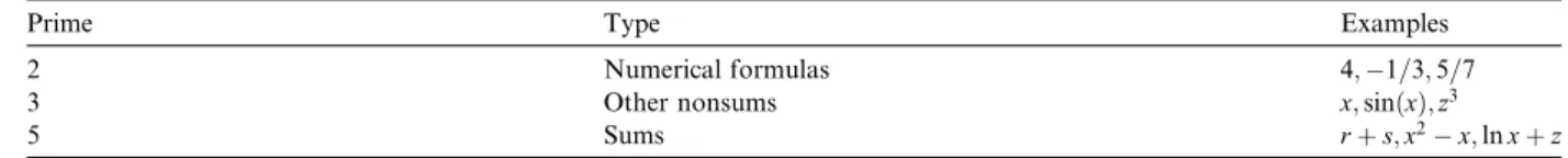
The kinds of subformulas that are distributed or factored from a formula can be precisely controlled by setting an appropriate value to the appropriate controller. Positive integer values cause distribution whereas negative values cause factoring. The exact type of formula which is distributed or factored can be determined fromTable 2.
If the value of the controllersnum_num, den_num, num_denorden_denis an integer multiple of one of
the primes listed inTable 2. Then formulas of the type associated with that prime are distributed (or factored if the controller is negative) in accordance with the transformations associated with that control variable.
• num_num– controls the distribution (factoring) of factors in the numerator of a formula over (from) the
terms of a sum in the numerator using the transformation:
a ðbþcÞ ¼abþac
Table 3has an example of the use of num_num to control the distribution of factors over a sum. Note that differences are internally represented as sums involving negative coefficients.
• den_den– controls the distribution (factoring) of factors in the denominator of a formula over (from) the
terms of a sum in the denominator using the transformation: 1
a ðbþcÞ 1
abþac
Table 2
Meaning of controllers
Prime Type Examples
2 Numerical formulas 4;1=3;5=7
3 Other nonsums x;sinðxÞ;z3
For example, ifden_denis 15, the formula
y x
1 1þx
1 1x
is transformed into
y xx3
• den_num– controls the distribution (factoring) of factors in the denominator of a formula over (from) the
terms of a sum in the numerator using the transformation:
bþc
a
b aþ
c a
For example, ifden_numis 6, the formula
xþ3 3
x
is transformed into
1 3þ
1
x
• num_den– controls the distribution (factoring) of factors in the numerator of a formula over (from) the
terms of a sum in the denominator using the transformation:
a bþc
1 b aþ
c a
This transformation yields a kind of continuation-fraction expansion. For example, ifnum_denis 5, the
formula 3þx
1þx
is transformed into 1
x
3þxþ
1 3þx
Ifnum_denis 30, the result is 1
1 1þ3
x þ 1
3þx Table 3
Transforming 3x ð1þxÞð1xÞwith different values for num_num
num_num Result
0 3x ð1þxÞð1xÞ
2 x ð1þxÞð33xÞ
3 3ð1þxÞðxx2Þ
5 3x ð1þxx ð1þxÞÞ
6 ð1þxÞð3x3x2Þ
10 x ð3þ3xþx ð33xÞÞ
15 3ðxx3Þ
References
[1] F. Winkler, Polynomial Algorithms in Computer Algebra, Springer-Verlag, 1996.
[2] B. Buchberger, G.E. Collins, R. Loos (Eds.), Computer Algebra, Symbolic and Algebraic Computation, second ed., Springer, 1983. [3] A.N. Whitehead, B. Russell, Principia Mathematica, vol. 1, Cambridge University Press, 1925, chapter Appendix 3.
[4] A. Diller, Compiling Functional Languages, John Willey & Sons Ltd, 1988. [5] B. Russel, Logic and Knowledge: Essays, George Allen & Unwin, 1956.
[6] C.E. Delaunay, The´orie du Mouvement de la Lune, 2 Vols., Mem. Acad. Sci., 28 and 29, Gauthier-Villars, Paris, 1867. [7] A. Deprit, J. Henrard, A. Rom, Ephemeris: Delaunay theory revisited, Science 168 (1970) 1569.
[8] N.J. Nilsson, Principles of Artificial Intelligence, Morgan Kaufman, 1980, pp. 35–47. [9] C.M. Chang, Mathematical Analysis in Engineering, Cambridge University Press, 1994.
[10] A. Hearn, Reduce: A user-oriented interactive system for algebraic simplification, in: M. Klerer, J. Reinfelds (Eds.), Interactive Systems for Experimental Applied Mathematics, Academic Press, 1968, pp. 79–80.
[11] F. Brackx, D. Constales, Computer Algebra with LISP and REDUCE, Kluwer Academic Publishers, 1992. [12] G. Andersson, Applied Mathematics with Maple, Chartwell-Bratt, 1997.
[13] D.C. Arney, Exploring Calculus with DERIVE, Addison-Wesley Publishing Company, 1992. [14] G.L. Bradley, K.J. Smith, Calculus, Prentice Hall, 1995.
[15] A.D. Andrew, G.L. Cain, S. Crum, T.D. Morley, Calculus Projects Using Mathematica, McGraw-Hill, 1996. [16] M. Scho¨nfinkel, Uber die Bausteine der mathematischen Logik, Mathematische Annalen 92, 305–316. [17] H.B. Curry, R. Feynes, Combinatory Logic, vol. 1, North-Holland, Amsterdam, 1958.
[18] A. Church, The calculi of lambda conversion, Annals of Math. Studies, vol. 6, Princeton University Press, Princeton, NJ, 1941. [19] S. Liang, P. Hudak, M. Jones, Monad transformers and modular interpreters, in: Conference Record of POPL’95: 22nd ACM
SIGPLAN- SIGACT Symposium on Principles of Programming Languages, San Francisco, CA, January 1995.
[20] M.P. Jones, S.P. Jones, Lightweight extensible records for haskell, in: Proceedings of the 1999 Haskell Workshop, October 1999. [21] J. Nordlander, Polymorphic subtyping in o’haskell, in: Proceedings of the APPSEm Workshop on Subtyping and Dependent Types in
Programming, Ponte de Lima, Portugal, 2000.
[22] S.P. Jones, S. Marlow, C. Elliott, Stretching the storage manager: weak pointers and stable names in haskell, IFL, 1999.