GENETIC ALGORITHMS APPLIED TO A FASTER DISTANCE
PROTECTION OF TRANSMISSION LINES
Denis V. Coury
∗M´
ario Oleskovicz
∗ [email protected]Silvio A. Souza
∗ [email protected]∗SEL-EESC-USP S˜ao Carlos
Av. Trabalhador Sancarlense. 400 Centro CEP 13566-590 - S˜ao Carlos – SP
RESUMO
Algor´ıtmos Gen´eticos Aplicados a uma Mais R´ a-pida Prote¸c˜ao de Distˆancia de Linhas de Trans-miss˜ao
O principal objetivo deste trabalho ´e implementar uma nova metodologia baseada em Algor´ıtmos Gen´eticos (AGs) para extra¸c˜ao de fasores fundamentais de tens˜ao e corrente em sistemas que possibilite uma prote¸c˜ao de distˆancia mais r´apida. Os AGs resolvem problemas de otimiza¸c˜ao baseados nos princ´ıpios da sele¸c˜ao natural. Esta aplica¸c˜ao foi formulada como um problema de oti-miza¸c˜ao, tendo como principal objetivo o de minimizar a estima¸c˜ao do erro entre as formas de ondas em an´alise. Uma linha de transmiss˜ao de 440 kV, com 150 km de extens˜ao foi simulada atrav´es dosoftwareATP ( Alterna-tive Transients Program) para testar a eficiˆencia do novo m´etodo. Os resultados desta aplica¸c˜ao mostram que o desempenho geral do AG foi altamente satisfat´orio no que diz respeito a velocidade e a precis˜ao na resposta quando comparado ao m´etodo tradicional utilizando a Transformada Discreta deFourier.
PALAVRAS-CHAVE: Prote¸c˜ao de Distˆancia, Transfor-mada Discreta de Fourier, Linhas de Transmiss˜ao e Al-gor´ıtmos Gen´eticos.
Artigo submetido em 23/02/2010 (Id.: 01106) Revisado em 20/08/2010, 09/12/2010
Aceito sob recomenda¸c˜ao do Editor Associado Prof. Julio Cesar Stacchini Souza
ABSTRACT
The main purpose of this paper is to implement a new methodology based on Genetic Algorithms (GAs) to ex-tract the fundamental voltage and current phasors from noisy waves in power systems to be applied to a faster distance protection. GAs solve optimization problems based on natural selection principles. This application was then formulated as an optimization problem, and the aim was to minimize the estimation error. A 440 kV, 150 km transmission line was simulated using the ATP (Alternative Transients Program) software in order to show the efficiency of the new method. The results from this application show that the global performance of GAs was highly satisfactory concerning speed and ac-curacy of response, if compared to the traditional Dis-crete Fourier Transform (DFT).
KEYWORDS: Distance Protection, Discrete Fourier Transform, Transmission Lines and Genetic Algorithms.
1
INTRODUCTION
and current signals are badly corrupted by noise, in the form of a DC offset (exponentially decaying transient), as well as harmonic components. Therefore, a protective relaying system has to detect them as soon as possible and isolate the faulty region from the rest of the system, preventing the propagation of the fault.
Many research groups have been working on digital pro-tection of transmission lines. Much attention has been paid to distance relaying techniques lately (Osman and Malik, 2001; Sidhu et al., 2002). Among many ap-proaches considered, transmission line protection based on the fundamental frequency signals is widely used. Ba-sically, the objective of a relaying scheme is to estimate the fundamental frequency components from the cor-rupted voltage and current signals following the fault oc-currence. For distance relaying, these fundamental com-ponents are used to determine the apparent impedance (Phadke and Thorp, 1988). According to the calculated impedance, the fault is identified as internal or external to the protection zone.
Some filtering techniques found in the literature can be applied to this problem. Various digital signal-processing techniques based on static and dynamic esti-mation have been suggested to evaluate the fundamental frequency (60 Hz). Some examples of static estimation are the Least-Squared Method (LSM) (Alfuhaid and El-Sayed, 1999) and the Discrete Fourier Transform (DFT) (Altuve et al., 1996). On the other hand, the Kalman Filter is an example of a dynamic estimation (Girgis and Brown, 1985). Genetic Algorithms (GAs) (Osman et al., 2003a; Macedo et al., 2003) and Artificial Neu-ral Networks (ANNs) (Osman et al., 2003b) have also been applied to the distance protection of power sys-tems. However, the DFT filter has been the most pop-ular for this purpose and has become a standard in the industry. This is because its computational cost is low and a good harmonic immunity can be reached. On the other hand, its performance can be adversely affected by the DC component leading to erroneous estimations, de-pending on the window length utilized. A shorter data window would give a faster response but an unstable output. A longer data window would give a stable re-sult, but the response of the filter would be delayed. For protection purposes, a data window of one cycle has been largely used (Chen et al., 2006).
The main purpose of this paper is to implement a new methodology based on GAs to extract the fundamen-tal voltage and current phasors in power systems to be applied to the distance protection. The optimization procedure follows an evolutionary strategy to find the best solution for a search problem. In order to obtain
a faster distance protection decision, the window length for the new methodology was analyzed in comparison to the standard DFT filter, showing some advantages concerning the new approach.
2
BASIC CONCEPTS RELATED TO
GE-NETIC ALGORITHMS
A Genetic Algorithm (GA) is a search algorithm based on the mechanism of natural selection and natural genet-ics. Its fundamental principle is “the fittest member of a population has the highest probability for survival”. A GA operates in a population of current approximations, the individuals, initially drawn in a random order, from which improvement is sought. Individuals are encoded as strings, the chromosomes, so that their values repre-sent a possible solution for a given optimization problem (Goldberge, 1989).
There is a fitness value associated to each chromosome. The better the solution the chromosome represents, the larger its fitness and its chances to survive and produce offspring. In this context, the objective function estab-lishes the basis of selection.
At the reproduction stage, a fitness value is derived from the raw individual performance measure given by the ob-jective function, as is used to bias the selection process. The selected individuals are then modified using genetic operators. Afterwards, individual chromosomes are de-coded, evaluated, and selected according to their fitness, and the process continues for different generations. By manipulating a population of possible solutions simulta-neously, the GAs can explore various areas of the search space.
The GAs rely on two basic kinds of operators: genetic and evolutionary. Genetic operators, namely crossover and mutation, are responsible for establishing how in-dividuals exchange or simply change their genetic fea-tures in order to produce new individuals. Evolutionary operators deal with determining which individuals will experience crossover or mutation.
3
THE REPRESENTATION OF THE
ES-TIMATION PROBLEM
3.1
The mathematical model of the input
signals
A periodic signal can be represented as a sum of its exponential DC, the fundamental frequency, as well as its harmonic components. In order to estimate the har-monic components of a nonsinusoidal waveform, a math-ematical expression can be written as (Pascual and Ra-pallini, 2001):
xe(t) =x0e−λ·t+ N
X
i=1
Ac,icos (iw0t) +As,isin (iw0t)
(1)
where x0 is the amplitude of the decaying DC compo-nent andλis its time constant; and are the cosine and sine amplitudes of theith harmonic respectively; is the fundamental frequency (377 rad/sec - 60 Hz) andN is the number of harmonics used to representx(t).
Assuming that the signal xs(t) is sampled at a pre-defined time interval ∆t, after (m−1)∗ ∆t seconds
there will be m samples, xs(t1), xs(t2). . . . .xs(tm), for
t1, t2. . . . .tm, where t1 is an arbitrary time reference. The system of equations given by equation (2), where
e(tk),k= 1. . . . .m, is the equation error at timetk, and can be written as:
xs(t1)
xs(t2) .. .
xs(tm)
=
e−λt1
· · · cos(N w0t1) sin(N w0t1)
e−λ2
· · · cos(N w0t2) sin(N w0t2) ..
. . .. ...
e−λtm
· · · cos(N w0tm) sin(N w0tm1)
· · x0
Ac,1
As,1 .. . Ac,N As,N +
e(t1)
e(t2) .. .
e(tm)
(2)
In this work, the system (2) is solved using GAs. Solving the system of equations given by (2), we would be able to find, λ, x0, and , i = 1, . . . , N. However,
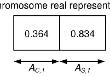
concern-ing the distance protection application, only the funda-mental phasors are required to calculate the apparent impedances seen by a local relay during a faulty situa-tion. Therefore, equation (1) was drastically simplified considering only the cosine and sine amplitudes of the fundamental component, and, respectively. Taking this into account, a real-coded GA scheme was used to repre-sent the cosine and sine amplitudes of the fundamental voltage and current, as illustrated in Figure 1. Consid-ering this approach, the GA worked as a filter for the voltage and current inputs, which is well known for be-ing corrupted by noise (as mentioned before).
0.364
0.834
A
C,1A
S,1Chromosome real representation
Figure 1: Individual representation.
3.2
The fitness function
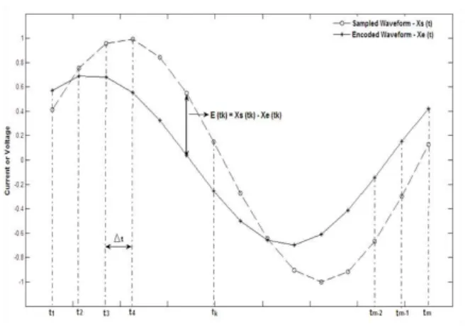
The evaluation function (FA) is responsible for deter-mining the fitness of each individual. Its objective is to evaluate the estimation error (e), in (3) . The coded pa-rameters in equation (2) are compared to the measured value in each time step in order to calculate the error (e) (Figure 2).
e(tk) =xs(tk)−xe(tk) k= 1...m (3)
The error represented in (4) was used in this work.
ET =
v u u u t m P i=1 ei m (4)
As the objective of the GAs is to maximize the chro-mosome’s fitness, it is necessary to transform ET into a fitness function (F). This is done using equation (5) , where ∆ is a very small positive constant, 0.00001, aimed to avoid overflow problems.
FA= 1
ET + ∆
(5)
Figure 2: The estimation error evaluation.
100 individuals, chromosomes with real representation, the tournament operator; the considered crossover and mutation rates of 90% and 10%, respectively. The stop criterion in each run was 5,000 generations or 100 gen-erations without improvement.
3.3
The Discrete Fourier Transform
Traditionally, the Fourier technique is widely used to analyze currents and voltage waveforms from an electric power system. In this work, the DFT technique is used in order to compare it to the new methodology proposed.
Considering the Fourier filter, the real and imaginary components of the fundamental frequency phasor (for one cycle of data with Nc samples per cycle), are given by the following equations (Pascual and Rapallini, 2001):
∧
x or= 2
N c
N c−1
X
n=0
x(n) cos
2π n N c
(6)
∧
x oi=− 2 N c
N c−1
X
n=0
x(n) sin
2π n N c
(7)
where and are the peak value of the real and imaginary components of the fundamental frequency phasor of the input signalx(n), respectively. For a half cycle and one quarter of a cycle,2/Ncshould be replaced by4/Ncand
8/Nc in equations (4) and (5) , respectively.
4
TEST RESULTS
4.1
Transmission line simulation
In order to obtain the voltage and current signals, which will be applied to distance protection, transmission lines with source equivalents at the ends were simulated (Fig-ure 3). This work makes use of a digital simulator of faulted EHV (Extra High Voltage) transmission lines known as the Alternative Transients Program - ATP (ATP, 1987).
A typical 440 kV transmission line, illustrated in Figure 4, from CESP (Companhia Energ´etica de S˜ao Paulo – a Brazilian utility) was utilized.
It should be mentioned that although the technique de-scribed is based on Computer Aided Design (CAD), practical considerations such as the Capacitor Voltage Transformer (CVT) and Current Transformers (CT), anti-aliasing filters and quantisation on system fault data were also included in the simulation. The data obtained was very close to that found in practice. The technique also considered the physical arrangement of the conductors in the structure (Figure 4), the char-acteristics of the conductors, mutual coupling, and the effect of earth return path. Perfect line transposition was assumed.
~
TL1 TL2 TL3~
80 km 150 km 100 km
10 GVA 9 GVA
D E F G
440 kV
Relay
ed using ATP software.
3 E 2
Figure 3: Power system simulated using ATP software.
The transmission line parameters are presented in Ta-ble 1. TaTa-bles 2 and 3 show the equivalent parameters concerning the generators and data fromD and G ter-minals, respectively.
For this approach, the voltage and current fault values from busbarE were utilised as inputs. A sampling fre-quency of 2.400 Hz to distance protection calculations was used.
11,93m
7,51m
24,07m 9,27m
0,40m
PHASE 1
PHASE 0
PHASE 3 PHASE 2
3,60m
Figure 4: Transmission line structure (440 kV).
Table 1: Transmission line parameters Positive Sequence
R (ohms/km) L (mH/km) C (uF/km)
3.853E-02 7.410E-01 1.570E-02
Negative Sequence
R (ohms/km) L (mH/km) C (uF/km)
1.861E+00 2.230E+00 9.034E-03
Table 2: Equivalent parameters fromD andGgeneration ter-minals
Generation TerminalD Positive Seq. Negative Seq.
R (ohms/km) 1.6982 0.358
L (mH/km) 5.14E+01 1.12E+01
Generation TerminalG Positive Seq. Negative Seq.
R (ohms/km) 1.7876 0.4052
L (mH/km) 5.41E+01 1.23E+01
Table 3: Data fromD andGGeneration Terminals Generation
TerminalD
Generation TerminalG
Power (GVA) 10 9
Voltage (pu) 1.05 0.95
Phase (grade) 0 -10
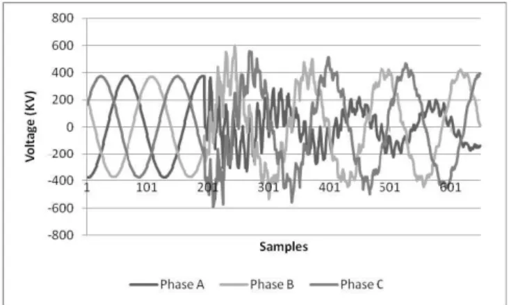
Figures 5 and 6 show a typical situation of an a-phase-to-earth fault in the TL2 transmission line at 75 km from busbar E.
Figure 5: Voltage waveforms at the TL2 transmission line.
Figure 6: Current waveforms at the TL2 transmission line.
The obtained data (voltage and current waveforms) were filtered using a 2ndorderButterworth filter with a cut-off frequency of 360 Hz in order to eliminate some of the high frequency components, as well as to prevent the aliasing effect. Moreover, the voltage and current wave-forms were digitalized using a 12 bit analog to digital converter (ADC).
4.2
Distance protection algorithm results
Impedance relays are from the family of distance relays. They are used to calculate the apparent impedance up to the fault point by measuring voltages and currents at one single end. As is known, they compare the apparent impedance/fault distance measured to a protection zone to determine if a fault is inside or outside it.
from the power system shown in Figure 3, simulated in the ATP software. The first step of the algorithm was the fault detection. Samples of current signals were stored in the memory. When a new sample came, it was compared to the corresponding sample one cycle earlier. If the change was bigger than 0,05 p.u and this change was confirmed by a counter four consecutive times, the fault situation was detected.
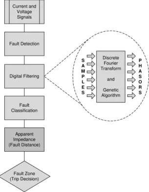
The next step was digital filtering. In this work, the tra-ditional DFT, as well as an alternative method, Genetic Algorithms (GA), were utilized in order to estimate the fundamental frequency phasors, as shown in 7 . Both methodologies were used to appropriately estimate these phasors as discussed in section 3.
The fault classification was also implemented because of the need to choose the voltages and currents involved in a fault adequately in order to correctly calculate the apparent impedance seen by the distance relay. The method adopted in the design consists of calculating the peak value of the three line currents and zero sequence current from the estimated states from the filters, as mentioned in Girgis and Brown (1985). Table 4 show the equations for fault impedance calculation according to the fault type (IEEE Std. C37.114T M, 2004).
Current and Voltage Signals
Fault Detection
Digital Filtering
Fault Classification
Apparent Impedance (Fault Distance)
Fault Zone (Trip Decision)
Discrete Fourier Transform
and
Genetic Algorithm
S A M P L E S
P H A S O R S
Figure 7. A basic diagram for a distance protection relay
Figure 7: A basic diagram for a distance protection relay.
In Table 4,A,BandCindicate the phases involved,Gis for ground,V andIare voltage and current phasors,k=
Table 4: Fault impedance equations for different types of faults.
Fault Type Equation
AG VA/(IA+ 3kI0)
BG VB/(IB+ 3kI0)
CG VC/(IC+ 3kI0)
ABorABG (VA−VB)/(IA−IB) BC orBCG (VB−VC)/(IB−IC) CAorCAG (VC−VA)/(IC−IA)
ABC The same as a phase-to-phase
(Z0˘Z1)/Z1, Z0andZ1correspond to zero and positive-sequence line impedance, respectively, andI0is the zero-sequence current.
Finally, after the apparent impedance calculation, that is proportional to the distance to the fault, the protected zone is inferred.
Considering the power system shown in Figure 3, all types of faults were simulated in order to test the pro-posed technique compared to the traditional DFT fil-tering method. For brevity, the results presented are concentrated in line-to-ground faults (AG) and phase-to-phase faults. The system behavior for the other fault types is similar to those presented.
These different kinds of faults were obtained considering the TL2 transmission line in Figure 3. The distances considered from busbarEwere: 15, 45, 75, 105, 135 and 145 km. The apparent impedances and fault distances were calculated for all kinds of faulty situations, taking into account not only the DFT but also the GA method. Windows of one, half and quarter of a cycle, i.e., 40, 20 and 10 samples from voltage and current waveforms were used as input for both methodologies. The fault inception angles for the simulations presented here were considered to be 0o
and 90o
. Moreover, fault resistances of 0, 50 and 100 Ohms were also included. Zone 1 was set to 80 % of the total line length. Consequently, fault distances of 15, 45, 75 and 105 km corresponded to the first zone and 135 and 145 km to the second zone.
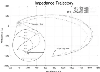
Figure 8 shows the impedance trajectory from the pre-to the post-fault data, considering the use of a DFT filter (one and half cycle windows), as well as a GA filter of a quarter cycle. A single line to ground (SLG) fault was located in the middle of the line with no fault resistance for this case study.
y for a SLG (AG) fault considering DFT and AG filters.
–
–
Figure 8: Impedance trajectory for a SLG (AG) fault considering DFT and AG filters.
figures as well as a representation for the positive se-quence line in question.
Figure 9 illustrates the estimated apparent impedances using both DFT and GA filters, considering the dis-tances described earlier along the line length versus the fault resistance variation for a single line to ground fault. The results show a good and correct estimation for both methods with one cycle data window.
Figure 10 illustrates the same situation using a half cycle data window. It can be observed that both methods presented similar results.
Finally, Figure 11 shows the same situation for a quar-ter cycle window. Considering the quarquar-ter cycle window of data, the use of GA shows a better result, especially because it kept the same type of response of the pre-vious cases. The same did not happen with the DFT technique, as already expected.
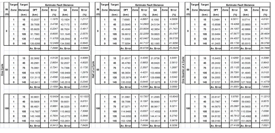
The fault distance estimations, as well as the zone in which the faults are located (1- inside the primary zone and 0- otherwise), for the cases illustrated in Figures 9, 10 and 11 are shown in Table 5. The results are shown in function of the error calculated according to 8:
e(%) =|destimated−dactual|
L ∗100 (8)
where, destimated is the fault distance estimated by the
GA; dactual is the actual fault distance; and L is the
total length of the transmission line.
It can be observed in Table 5 that generally the GA methodology shows a better performance (in terms of
errors) if compared to the DFT method. This can be better observed in the cases using a quarter data win-dow. For these cases, the fault distance estimations, as well as location zones, were on average much more precise, if compared to the traditional method, provid-ing better conditions to the new method to distprovid-inguish different relay zones with this very short window.
–
–
Figure 9: R – X diagram for a SLG (AG) fault with 0, 50 and 100 Ohms fault resistances and one cycle data window.
–
– Figure 10: R – X diagram for a SLG (AG) fault with 0, 50 and 100 Ohms fault resistances and half cycle data window.
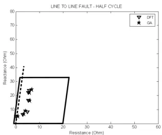
Figure 12 presents a R – X diagram for a double line fault (AB) with fault resistance of 1 Ohm, considering a one cycle data window. A good estimation for both methods can be seen.
Figure 13 shows the same situation for a half cycle data window. Once more, both methods had approximately the same performance.
–
–
–
Figure 11: R – X diagram for a SLG (AG) fault with 0, 50 and 100 Ohms fault resistances and quarter cycle data window.
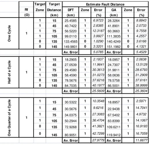
observed considering the GA technology. This behavior can also be found considering the distance estimations presented in Table 6 where the GA technique with a quarter cycle data window presented much smaller av-erage errors if compared to the DFT.
It must be emphasized that, the GA methodology can present different results depending on its initialization. Considering this, in order to have a realistic result, each test was run individually 30 times and its average per-formance is presented in the tables.
The average running times for the proposed algorithm, considering fault detection, classification and location are 19.17 ms, 10.84 ms and 6.67 ms considering one, half and quarter cycle data windows, respectively.
–
–
Figure 12: R – X diagram for a double line (AB) fault with 1 Ohm fault resistance and one cycle data window.
–
–
–
Figure 13: R – X diagram for a double line (AB) fault with 1 Ohm fault resistance and half cycle data window.
– Figure 14: R – X diagram for a double line (AB) fault with 1Ohm fault resistance and quarter cycle data window.
4.3
Practical implementation
This work has been developed on a simulation basis. However, it should be mentioned that an embedded methodology using FPGAs (Field-Programmable Gate Arrays) would be very suitable for this application. The system on chip concept makes intelligent digital distance relays possible in practice. A similar approach was im-plemented in Souza et al. (2008) for on-line applica-tion of a frequency relay (estimating frequency devia-tion, phasor magnitude and phase angle) with very good results, facing all the restraints concerning an on-line re-lay application.
5
CONCLUSIONS
This work presented an efficient technique based on Ge-netic Algorithms applied to distance protection of power systems. Considering the study, the proposed method-ology performed better compared to the traditional Dis-crete Fourier Transform method.
A basic algorithm for distance protection was tested and situations such as different types of faults, fault resis-tances, fault distances and size of the input data window were considered.
It can be concluded that the size of the window is very important for a good estimation. As far as distance protection is concerned, a shorter data window would give a faster response. In this context, the deprecia-tion of the results when the size of the data window was made shorter could particularly be observed in the case of the DFT technique. The use of one, half and quarter cycle data windows showed an interesting com-parison between the Genetic Algorithm and Discrete Fourier Transform with better performances in favor of the GA methodology. This is particularly important if we have in mind the times normally required for com-mercial relays (between one and two cycles) concerning the fault detection, classification and location for trans-mission lines.
ACKNOWLEDGEMENT
The authors acknowledge the Department of Electrical Engineering – Engineering School of S˜ao Carlos - Uni-versity of S˜ao Paulo (Brazil), for the research facilities provided to conduct this project. Our thanks also to FAPESP -Funda¸c˜ao de Amparo `a Pesquisa do Estado de S˜ao Paulo for the financial support.
REFERENCES
Alfuhaid, A. S. and El-Sayed, M. A. (1999). A re-cursive least-squares digital distance relaying algo-rithm. IEEE Trans. Power Delivery, v. 14, n. 4, pp. 1257-1262.
Altuve, F. H. J.; Diaz, V. and Vazquez, M. E. (1996). Fourier and Walsh digital filtering algorithms for distance protection. IEEE Trans. Power Delivery, v. 11, n. 1, pp. 457-462.
ATP (1987). Alternative Transient Program. Leuven EMTP Center – Rule Book.
Chen, C. S.; Liu, C. W. and Jiang, J. A. (2006). Appli-cation of combined adaptive Fourier filtering
tech-nique and fault detector to fast distance protection.
IEEE Trans. Power Delivery, v. 21, n. 2, pp. 619-626.
Girgis, A. A. and Brown, R. G. (1985). Adaptive Kalman filtering in computer relaying: fault classi-fication using voltage models. IEEE Trans. Power Apparatus Systems, v. 104, n. 5, pp. 1167-1177.
Goldberge, D. (1989). Genetic algorithms in search. in: optimization and machine learning. Addison-Wesely.
IEEE Std. C37.114T Mm (2004). IEEE Guide for de-termining fault location on AC transmission and distribution lines. IEEE Publish, New York.
Macedo, R. A.; Silva, D. F.; Coury, D. V. and Carneiro, A. A. F. M. (2003). An evolutionary optimization approach to track voltage and current harmonics in electrical power systems. IEEE Power Eng. Soc. Gen. Meet., v. 2, pp. 1250-1255.
Osman, A. H. and Malik, O. P. (2001). Wavelet trans-form approach to distance protection of transmis-sion lines. IEEE Power Eng. Soc. Summer Meet., 1, pp. 15-19.
Osman, A. H.; Abdelazim, T. and Malik, O. P. (2003a). Genetic algorithm approach for adaptive data win-dow distance relaying. IEEE Power Eng. Soc. Gen. Meet., v. 3, pp. 1862-1867.
Osman, A. H.; Abdelazim, T. and Malik, O. P. (2003b). Adaptive distance relaying technique using on-line trained neural network. IEEE Power Eng. Soc. Gen. Meet., v. 3, pp. 13-17.
Pascual, H. O. and Rapallini, J. A. (2001). Behaviour of Fourier, cosine and sine filtering algorithms for distance protection, under severe saturation of the current magnetic transformer. IEEE Porto Power Tech Conf.
Phadke, A. G. and Thorp, J. S. (1988). Computer Relaying for Power Systems. John Wiley & Sons.
Sidhu, T. S.; Ghotra, D. S. and Sachdev, M. S. (2002). An adaptive distance relay and its performance comparison with a fixed data window distance re-lay. IEEE Trans. Power Delivery, v. 17, n. 3, pp. 691-697.
T ab le 5 : Di st an ce es tim at io n fo r a S L G (A G ) fa u lt w ith o n e, h alf an d q u ar te r d at a w in d ow s.
Table V. Distance estimation for a SLG (AG) fault with one, half and quarter data windows.
Target Target Target Target Target Target
Rf Zone Distance DFT Zone Error GA Zone Error Rf Zone Distance DFT Zone Error GA Zone Error Rf Zone Distance DFT Zone Error GA Zone Error
(Ω) (km ) (km ) (%) (km ) (%) (Ω) (km ) (km ) (%) (km ) (%) (Ω) (km ) (km ) (%) (km ) (%)
1 15 13.2037 1 1.1975 13.1824 1 1.2117 1 15 7.6565 1 4.8957 8.1092 1 4.5939 1 15 5.2484 1 6.5011 8.0714 1 4.6191
1 45 39.7938 1 3.4708 43.7172 1 0.8552 1 45 23.5645 1 14.2903 24.5134 1 13.6577 1 45 15.8598 1 19.4268 23.9893 1 14.0071
1 75 65.6629 1 6.2247 66.7624 1 5.4917 1 75 40.4049 1 23.0634 42.3854 1 21.7431 1 75 23.8415 1 34.1057 42.6866 1 21.5423
1 105 91.7993 1 8.8005 101.1645 1 2.5570 1 105 56.6612 1 32.2259 59.8820 1 30.0787 1 105 33.6484 1 47.5677 62.3094 1 28.4604
0 135 117.4943 1 11.6705128.2942 0 4.4705 0 135 71.9300 1 42.0467 75.6420 1 39.5720 0 135 38.3164 1 64.4557 73.8130 1 40.7913
0 145 126.6266 0 12.2489134.5082 0 6.9945 0 145 77.9294 1 44.7137 82.1065 1 41.9290 0 145 41.2405 1 69.1730 85.9315 1 39.3790
Av. Error 7.2688 Av. Error 3.5968 Av. Error 26.8726Av. Error 25.2624 Av. Error 40.2050Av. Error 24.7999
1 15 22.3692 1 4.9128 22.3633 1 4.9089 1 15 21.6517 1 4.4345 21.9736 1 4.6491 1 15 15.6403 1 0.4269 21.5082 1 4.3388
1 45 49.2981 1 2.8654 52.2037 1 4.8025 1 45 46.4780 1 0.9853 48.8420 1 2.5613 1 45 26.2432 1 12.5045 43.5535 1 0.9643
1 75 76.0861 1 0.7241 74.7398 1 0.1735 1 75 71.4740 1 2.3507 73.0954 1 1.2697 1 75 37.3313 1 25.1125 65.6395 1 6.2403
1 105 104.1978 1 0.5348 106.9469 1 1.2979 1 105 98.3654 1 4.4231 103.4606 1 1.0263 1 105 45.3913 1 39.7391 91.4845 1 9.0103
0 135 131.3115 0 2.4590 133.6485 0 0.9010 0 135 125.3974 0 6.4017 129.6986 0 3.5343 0 135 54.2055 1 53.8630 114.5856 1 13.6096
0 145 142.8411 0 1.4393 145.3518 0 0.2345 0 145 135.0332 0 6.6445 137.0275 0 5.3150 0 145 57.5727 1 58.2849 127.7832 0 11.4779
Av. Error 2.1559 Av. Error 2.0530 Av. Error 4.2066 Av. Error 3.0593 Av. Error 31.6551Av. Error 7.6069
1 15 30.9651 1 10.6434 30.1534 1 10.1023 1 15 31.0961 1 10.7307 31.2065 1 10.8043 1 15 23.8147 1 5.8765 31.8320 1 11.2213
1 45 59.5809 1 9.7206 59.8051 1 9.8701 1 45 58.7096 1 9.1397 58.9060 1 9.2707 1 45 33.7967 1 7.4689 59.9363 1 9.9575
1 75 88.4821 1 8.9881 88.3220 1 8.8813 1 75 87.3271 1 8.2181 88.9817 1 9.3211 1 75 44.5670 1 20.2887 84.5603 1 6.3735
1 105 116.7607 1 7.8405 115.9602 1 7.3068 1 105 114.9460 1 6.6307 117.4552 1 8.3035 1 105 55.9241 1 32.7173 115.5594 1 7.0396
0 135 145.1406 0 6.7604 143.0772 0 5.3848 0 135 144.0050 0 6.0033 144.4114 0 6.2743 0 135 64.8132 1 46.7912 140.4982 0 3.6655
0 145 154.1422 0 6.0948 153.2651 0 5.5101 0 145 153.1298 0 5.4199 153.9517 0 5.9678 0 145 68.0160 1 51.3227 151.0829 0 4.0553
Av. Error 8.3413 Av. Error 7.8426 Av. Error 7.6904 Av. Error 8.3236 Av. Error 27.4109Av. Error 7.0521
0
50
100 Estim ate Fault Distance
O n e C y c le 0 50 100 H a lf o f a C y c le 0 O n e Q u a rt e r o f a C y c le 50 100
Estim ate Fault Distance Estim ate Fault Distance
Table 6: Distance estimation for a double line (AB) fault with one, half and quarter data windows.
Target Target
Rf Zone Distance DFT Zone Error GA Zone Error
(Ω) (km ) (km ) (%) (km ) (%)
1 15 25.4585 1 6.9723 28.3264 1 8.8843
1 45 40.7422 1 2.8385 41.8901 1 2.0733
1 75 56.5220 1 12.3187 60.3663 1 9.7558
1 105 99.0110 1 3.9927 111.3835 1 4.2557
0 135 133.4565 0 1.0290 140.4249 0 3.6166
0 145 149.9801 0 3.3201 151.1982 0 4.1321
Av. Error 5.0785 Av. Error 5.4529
1 15 18.2905 1 2.1937 18.0957 1 2.0638
1 45 27.0539 1 11.9641 24.7307 1 13.5129
1 75 29.4580 1 30.3613 31.9811 1 28.6793
1 105 58.4590 1 31.0273 58.0636 1 31.2909
0 135 78.5676 1 37.6216 78.5758 1 37.6161
0 145 84.7035 1 40.1977 86.5001 1 38.9999
Av. Error 25.5609 Av. Error 25.3604
1 15 30.5322 1 10.3548 18.8957 1 2.5971
1 45 30.5676 1 9.6216 22.9438 1 14.7041
1 75 34.0375 1 27.3083 67.5402 1 4.9732
1 105 50.2944 1 36.4704 83.8399 1 14.1067
0 135 72.9268 1 41.3821 109.6211 1 16.9193
0 145 80.9051 1 42.7299
119.9412 1 16.7059
Av. Error 27.9779 Av. Error 11.6677
Estim ate Fault Distance
1
1 1
O
n
e
C
y
c
le
H
a
lf
o
f
a
C
y
c
le
O
n
e
Q
u
a
rt
e
r
o
f
a
C
y
c