Braz. J. Phys. vol.35 número4B

Statefinder Revisited

´

Emille E. O. Ishida

Universidade Federal do Rio de Janeiro, Instituto de F´ısica, CEP 21941-972, Rio de Janeiro, RJ, Brazil

(Received on 3 October, 2005)

The quality of supernova data will dramatically increase in the next few years by new experiments that will add high-redshift supernova to the currently known ones. In order to use this new data to discriminate between different dark energy models, the statefinder diagnostic was suggested [1] and investigated by Alamet al.[3] in the light of the proposed SuperNova Acceleration Probe (SNAP) satellite. By making use of the same procedure presented by these authors, we compare their analyzes with ours, which shows a more realistic supernovae redshift distribution and do not assume that the intercept is known. We also analyzed the behavior of the statefinder pair{r,s}and the alternative pair{s,q}in the presence of offset errors.

Introduction

Recent observations from type Ia supernovae measure-ments, cosmic microwave background radiation and gravita-tional clustering suggest the expansion of the universe is ac-celerated.

In order to explain this cosmic acceleration a form of negative-pressure matter called dark energy was suggested. The simplest and most popular candidate is Einstein’s cosmo-logical constant. Many others candidates for dark energy have been proposed, including scalar fields with a time dependent equation of state, quartessence, modified gravity, branes, etc. Confrontation between these models and currently observa-tional data doesn’t say much [2], mainly because most of them haveΛCDM as a limiting case in the redshift range already observed. The SNAP (SuperNovae Acceleration Probe) satel-lite is expected to observe∼2000 supernovae per year with redshift up toz=1.7. To differentiate models using the new available data, Sahniet al. [1] introduced thestatefinder di-agnostic, that is based on the dimensionless parameters{r,s}, which are constructed with the scale factor and its time deriv-atives.

In this work we applied the statefinder to a SNAP-like su-pernovae distribution and analyzed its behavior in the pres-ence of systematic and random systematic, beyond statistical errors.

I. DARK ENERGY MODELS

Assuming a Friedman-Robertson-Walker (FRW) metric, the Einstein’s equations reduce to:

H2 = 8πG

3

∑

kc2

a2 (1)

¨

a

a = −

4πG

3

∑

pi

c2) (2)

whereais the scale factor of the FRW metric,His the Hubble parameter, and the sum is over all the components present in the scenario in study.

In the following we assume that the matter content of the universe is given by dark matter (pm =0) and dark energy with an equation of state in the form px=px(ρx). We also takec=1 and consider a flat universe (k=0).

The focus of our discussion will be in the four models listed below:

1. Cosmological Constant(wx=px/ρx=−1)

The cosmological constant model represents a constant energy density. In this model, the Hubble parameter has the form:

H(z) =H0[Ωm0(1+z)3+1−Ωm0] 1

2 ₍₃₎

2. Quiessence (−1/3>wx=px/ρx=cte>−1) This is the next simplest example of dark energy model, and gives rise to a Hubble parameter like:

H(z) =H0[Ωm0(1+z)3+ΩX0(1+z)3(1+w)] 1 2 ₍₄₎

3. Quintessence( w = w ( t ) )

Representing a self-interacting scalar field minimally coupled to gravity. In this model, we have:

ρφ = 1

2φ(z)˙

2_+V(φ(z))

(5)

pφ = 1

2φ(z)˙

2_{−V(φ(z)) (6)}

We shall focus on a special kind of quintessence model that has atrackerlike solution, with the following po-tential: V(φ) =φ(z)−α(α>0). In this case, it can be shown that the present energy density of the dark en-ergy is almost independent of initial conditions.

4. Chaplygin Gas

A different kind of solution is provided by the Chap-lygin gas model. In this model, the Hubble parameter takes the form:

H(z) =H0 ·

Ωm0(1+z)3+Ω_κmo r

A

B+ (1+z) 6

¸1₂

(7) where

κ=_ρρmo ch0

TABLE I: Redshift distribution. The value of z represent the upper edge of each bin [4]

z 0.1 0.2 0.3 0.4 0.5 0.6 0.7 0.8 0.9 1.0 1.1 1.2 1.3 1.4 1.5 1.6 1.7

N(z) 0 35 64 95 124 150 171 183 179 170 155 142 130 119 107 94 80

It is important to note that for all models presented previ-ously, the luminosity distance is :

DL(z) 1+z =

Z z

0 dz′

H(z′₎ (9)

with H(z) given by the model dependent expressions pre-sented before.

II. THE STATEFINDER

The properties of dark energy, as we have seen, are very model dependent. In order to differentiate between the pre-sented models, Sanhiet al.[1], proposed the statefinder diag-nostic. The parameters, {r,s}, are a complement to the al-ready known deceleration parameter, and help the discrimina-tion when the later contains degeneracies. By definidiscrimina-tion:

q=− a¨ aH2≡

1

2(1+3wΩX) (10)

r≡ a¨

aH3=1+

9w

2 ΩX(1+w)− 3 2ΩX

˙

w

H (11)

s≡ r−1 3(q−1

2)

=1+w−1 3

˙

w

wH (12)

III. DARK ENERGY FROM SNAP DATA

Type Ia supernovae are considered standard candles, used to map the expansion history, and its observations lead to the behavior of the scale factor with time. In order to study the data in a model independent way, we use a parametrization for the dark energy density, presented by Sahniet al. [1]. We express the energy density as a power series up to second order in z: ρDE=ρc0(A1+A2x+A3x2), wherex=1+z. For this Ansatz, the Hubble parameter takes the form:

H(x) =H0(Ωm0x3+A1+A2x+A3x2) 1

2 ₍₁₃₎

equation (13) together with equation (9) provides an expres-sion for the luminosity distance, which we shall investigate, using the statefinder parameters, in the light of a SNAP-like experiment simulation.

To simulate the data, we use a binned approach for a SNAP distribution shown in the Table I. We also include 300 su-pernovae in the first bin. These low redshift susu-pernovae are expected from the SNFactory (Nearby Supernovae Factory) experiment and are important in reducing the systematic er-rors. The SNFactory proposal is to provide data to calibrate high redshift experiments, like the SNAP, and then reduce the errors involved.

The luminosity distance of equation (9) is measured in terms of the apparent magnitude, which can be written as:

m(z) = 5 logDL(z) +

[M+25−5 log(H0/(100km/s/M pc))] (14) where M is the absolute magnitude of the supernova and the expression in brackets is calledintercept.

Following what was done by Kimet al. [4], we consider a random irreducible systematic error of 0.04∗(zmed/1.7)(here zmedis the redshift in the middle of each bin), added in quadra-ture to a constant statistical error of 0.15magand study the behavior of the statefinder parameter with this synthetic data. We performed a Monte Carlo simulation considering the in-tercept exactly known and totally unknown. As a second step, we study the situation where offset errors are present, and its consequences in the statefinder.

IV. RESULTS

In the figures 1 to 9 we present the results from simulated data. According to SNAP’s specifications, we generated 500 data sets havingΛCDM as a fiducial model. For each of this experiments we calculated the best fitting parametersA1and

A2for equation (13) and reconstructed the statefindersr(z)e

s(z). The figures below show the mean value of the parame-ters, which were calculated as:

<(r)> = 1

500

500

∑

ri(z) (15)

<(s)> = 1

500

500

∑

si(z) (16)

<(q)> = 1

500

500

∑

qi(z) (17)

0.25 0.5 0.75 1 1.25 1.5 z

0.25 0.5 0.75 1 1.25 1.5 1.75 2

<

r

>

w= -0.8 w= -0.6

k=2 k=1

Α=2

Α=4

CHAPLYGIN GAS

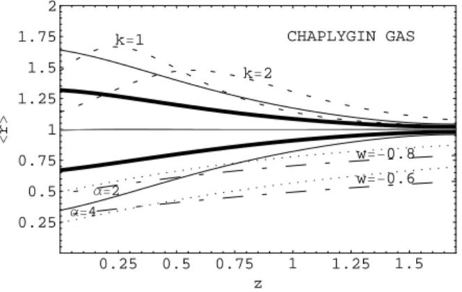
FIG. 1: Shows<r>as a function of redshift. The dark black contour represent 1σand the full line 2σconfidence levels, in the presence of statistical

errors with a known intercept.The line<r>=1 (gray line) represents theΛCDM fiducial model. The dashed lines above theΛCDM are Chaplygin gas with

parametersk=1 andk=2. The dotted lines below it are quiessence models withw=−0.6 andw=−0.8, and the dotted-dashed lines are quintessence models

withα=2 andα=4.

0.25 0.5 0.75 1 1.25 1.5 z

0.25 0.5 0.75 1 1.25 1.5 1.75 2

<

r

>

w=-0.8

w=-0.6 k=2

k=1

Α=2

Α=4

CHAPLYGIN GAS

FIG. 2:Analog to figure 1, but here in the presence of random systematic and statistical errors, with an unknown intercept.

0.25 0.5 0.75 1 1.25 1.5 z

0.25 0.5 0.75 1 1.25 1.5 1.75 2

<

r

>

w= -0.8 w= -0.6

k=2 k=1

Α=2

Α=4

CHAPLYGIN GAS

FIG. 3:Shows<r>as a function of redshift. Again, the dark and full contours are 1σand 2σconfidence levels, in these we considered a known intercept in

the presence of statistical error and a systematic error of+0.03mag.The dotted, dot-dashed and dashed lines are the same as in figure 1.

0.25 0.5 0.75 1 1.25 1.5 z

-0.75 -0.5 -0.25 0 0.25 0.5 0.75 1

<

s

>

k= 1 k= 2 w=-0.6

w=-0.8

Α=4

Α=2

CHAPLYGIN GAS

0.25 0.5 0.75 1 1.25 1.5 z

-0.75 -0.5 -0.25 0 0.25 0.5 0.75 1

<

s

>

k= 1 k= 2

w=-0.6

w=-0.8

Α=2

CHAPLYGIN GAS

Α=4

FIG. 5:Analog to figure II, but here in the presence of random systematic and statistical errors, with an unknown intercept.

0.25 0.5 0.75 1 1.25 1.5 z

-0.75 -0.5 -0.25 0 0.25 0.5 0.75 1

<

s

>

k= 1 k= 2 w=-0.6

w=-0.8

Α=4

Α=2

CHAPLYGIN GAS

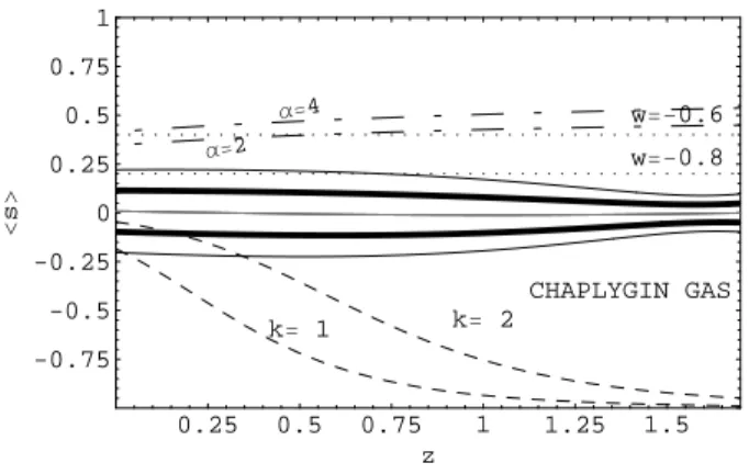
FIG. 6:Shows<s>as a function of redshift. Again, the dark and full contours are 1σand 2σconfidence levels, in this we considered a known intercept in the

presence of statistical error and a systematical errors of+0.03mag.The dotted, dot-dashed and dashed lines are the same as in figure 1.

0.25 0.5 0.75 1 1.25 1.5 z

-0.75 -0.5 -0.25 0 0.25 0.5 0.75 1

<

q

>

Α=2

k=1

k=2 Α=4

FIG. 7:Shows<q>as a function of redshift. The dark contour represent 1σand the full lines 2σconfidence levels. The dashed lines are Chaplygin gas with

parametersk=1 andk=2. The dotted-dashed lines are quintessence models withα=2 andα=4.

0.25 0.5 0.75 1 1.25 1.5 z

-0.75 -0.5 -0.25 0 0.25 0.5 0.75 1

<

q

>

k=1

k=2

Α=2

Α=4

0.25 0.5 0.75 1 1.25 1.5 z

-0.75 -0.5 -0.25 0 0.25 0.5 0.75 1

<

q

>

Α=2

k=1

k=2 Α=4

FIG. 9:Shows<q>as a function of redshift. Again, the dark contour and full line are 1σand 2σconfidence levels, in these we considered a known intercept

in the presence of statistical error and a systematical error of+0.03mag.The dot-dashed and dashed lines are the same as in figure 7.

0.2 0.4 0.6 0.8 1 1.2 1.4 r

 -1

-0.5 0 0.5 1

s



w=-0.9 w=-0.7 w=-0.5 w=-0.33

w=-0.0

k=37 k=1 k=2 k=6 k=15

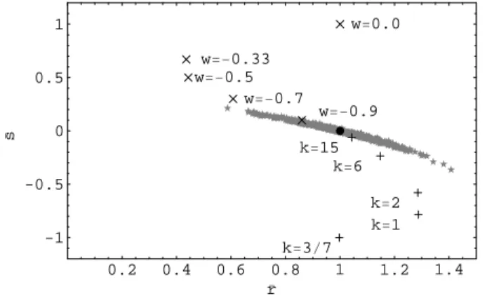
FIG. 10: Shows the variation of ¯rwith ¯s, in the presence of statistical error when the intercept is known. The black circle is theΛCDM fiducial model.

The points marked with ”X” above theΛCDM are quiessence models withw=0.0,−0.3,(−0.5),−0.7 and 0.9 respectively, from top to bottom. The points

represented by ”+” belowΛCDM are Chapligyn gas withk= (3/7),1,2,6,15, from bottom to top.

0.2 0.4 0.6 0.8 1 1.2 1.4 r

 -1

-0.5 0 0.5 1

s



w=-0.9 w=-0.7

w=-0.5 w=-0.33

w=0.0

k=37 k=1 k=2 k=6 k=15

FIG. 11:This is analogous to figure 10, although here we considered an intercept not known and included statistical and random systematic errors.

0.2 0.4 0.6 0.8 1 1.2 1.4 r

 -1

-0.5 0 0.5 1

s



k=37 k=1 k=2 k=6 k=15

w=-0.9 w=-0.7 w=-0.5 w=-0.33

w=-0.0

FIG. 12:Show the variation of ¯rwith ¯swhen the intercept is known, in the presence of statistical error and systematic error of+0.03mag. The circle, ”X” and

-0.4 -0.2 0 0.2 0.4 0.6 0.8 s

 -1

-0.5 0 0.5 1

q



k=37 k=1 k=2 k=6 k=15

w=-0.9 w=-0.7

w=-0.5 w=-0.33

w=-0.0

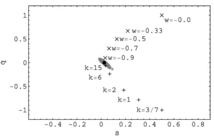
FIG. 13: Shows the variation of ¯swith ¯q, in the presence of statistical error when the intercept is known. The circle is theΛCDM fiducial model. The ”X”

points above theΛCDM are quiessence models withw=0.0,−0.3,(−0.5),−0.7 and 0.9 respectively, from top to bottom. The ”+” points belowΛCDM are

Chapligyn gas withk= (3/7),1,2,6,15, from bottom to top.

-0.4 -0.2 0 0.2 0.4 0.6 0.8 q



-1 -0.5 0 0.5 1

s



w=-0.9 w=-0.7

w=-0.5 w=-0.33

w=0.0

k=37 k=1 k=2 k=6 k=15

FIG. 14:This is analogous to figure 13, although here we considered an intercept not known and included statistical and random systematic errors.

-0.4 -0.2 0 0.2 0.4 0.6 0.8 q

 -1

-0.5 0 0.5 1

s



w=-0.9 w=-0.7

w=-0.5 w=-0.33

w=-0.0

k=37 k=1

k=2 k=6 k=15

¯

r = 1

zmax

Z zmax

0 r(z)dz (18)

¯

s = 1

zmax

Z zmax

0

s(z)dz (19)

¯

q = 1

zmax

Z zmax

0 q(z)dz (20)

wherezmax=1.7 . The expressions forr, sandqwere calcu-lated using equations 13, 11 and the first part of equation 12 for each experiment. The 500 points obtained are plotted in figures 10 to 15.

V. DISCUSSION

Our results suggest that the statefinder is a good diagnostic for dark energy models, although some care must be taken in applying it to data. As expected, the presence of random systematic error and an unknown intercept just added more possible models than those allowed by statistical errors only. There is little problem in this, once the fiducial model is at least within the 2σcontours (Figures 2, 5 and 8).

The presence of offset errors had different outcomes. For a positive offset, the parametersrandssuffered a small reduc-tion in relareduc-tion to the fiducial model, but in different redshift ranges (r for small and s for high redshift). A consequence

of this arises when we compare the integrated averages of the pair{r,s}. In Figure 12 the points are shifted to the negative direction of both axes of the ellipse, resulting a data set where the fiducial model (red point) is on the edge of the distribution. The same kind of shift is observed for a negative offset, but in this case to the positive direction of the axes. So, in order to use the statefinder as a diagnostic, we must be able to control the offset error below 0.03mag.

It is interesting to observe the behavior of the decelera-tion parameter when systematic errors were involved. It does present a very small reduction (positive offset) at high red-shift, but it is irrelevant in front of that suffered byr or s. Comparing figures 10 and 13 we could say, as suggested by Alamet al. [3], that the pair{q,s}is even a better diagnostic than{r,s}, once it restricts the area of the phase space filled by the data. However, if there is a systematic error present, the points will be shifted to the negative direction of theqaxis only (figure 15), letting the distance between the data and the fiducial model bigger than those in figure 12.

Therefore, we concluded that the statefinder pair{r,s}is a better diagnostic than the pair{s,q}, when the involved sys-tematic errors are not random.

Acknowlegments

The author is grateful to Ioav Waga for suggesting this problem and for extensive discussion and encouragement throughout the course of the work. This work was supported by the Brasilian research agency CNPq.

References

[1] V. Sahni, T. D. Saini, A. A. Starobinsky, and U. Alam, JETP Lett.77, 201 (2003)

[2] K. D. Evans , I. K. Wehus , O. Gron, and O. Elgaroy, Astron. Astrophys.430, 399 (2005)

[3] U. Alam, V. Sahni , T. D. Saini, and A. A. Starobinsky, Mon.Not.Roy.Astron.Soc.344, 1057 (2003)

[4] A. G. Kim, E. V. Linder, R. Miquel and N. Mostek, Mon.Not.Roy.Astron.Soc.347, 909 (2004)