Braz. J. Phys. vol.34 número4B

Brazilian Journal of Physics, vol. 34, no. 4B, December, 2004 1673

Determination of Plasma Temperature by a Semi-Empirical Method

F. O. Borges, G. H. Cavalcanti, and A. G. Trigueiros

Laborat´orio de Plasma e Espectroscopia, Instituto de F´ısica, Universidade Federal Fluminense, UFF Campus da Praia Vermelha-Gragoat´a, 24210-340 Niter´oi, Rio de Janeiro, Brazil

Received on 26 January, 2004; revised version received on 28 April, 2004

Doppler or Stark line broadening effects are generally used to determinate plasma temperature. These methods are difficult to apply to spectra of highly ionized atoms due to the short wavelengths involved. It is not at all easy to achieve sufficient wavelength resolution in this spectral range. In this case, a spectroscopic technique based on the relative intensities of lines must be used to measure the electron temperature in a plasma. However the relation of the measure of relative line intensity and the plasma electron temperature is complex and a number of issues must be examined for the diagnostic. In simple cases, only a two levels system need be considered. Here we introduce a semi-empirical method to determine the plasma temperature that takes into account multiple levels structure. In the theoretical model we consider alocal thermodynamic equilibrium(LTE). The greatest difficult in the determination of plasma temperature using a multiple levels approach is overcome by calculating the transition probabilities in terms of the oscillator strength parameters. To check the method we calculated the oscillator strengths for the Cu I using a multi-configurational Hartree-Fock relativistic (HFR) approach. The electrostatic parameters were optimized by a least-squares procedure, in order to obtain the best fitting to the experimental energy levels. This method producesgf-values that are in better agreement with their experimental values than the produced by theab initiocalculation. The temperature obtained was 5739.3 K, what is compatible with direct measurements made for cupper DC discharge.

1

Determination of plasma

tempera-ture

The plasma temperature may be estimated through the relative emission intensities of spectral lines. From the the-ory of atomic structure and spectra [1], the relative intensi-ties of the spectral lines, considering a Boltzmann distribu-tion, are given by the equation

ln

µ_Iλ3

gf

¶

=− Eu

kBT

+constant=−aEu+b, (1)

whereI,λandf are the relative intensity, wavelength, and oscillator strength respectively. Euis the energy of the

up-per level andgis the statistic weight of the lower level;kBis

the Boltzmann constant,T is the temperature andba cons-tant parameter for all ion lines considered. In a few cases,

g,f andEucan be obtained from the handbook of the

spec-troscopic constants, chemistry and physics.

The equation(1) gives the plasma temperature in the case of LTE approximation. To increase the precision a large number of spectral lines must be used to determine plasma temperature. For a given spectrum, a plot of the logarith-mic term in the right hand of equation(1) versusEu yields

a straight line whose slope is equal to1/kBT. Thus we can

obtain the plasma temperature from the slopea. Using

T = 1

kBa

. (2)

We apply the above mentioned method to some copper lines which spectroscopic constants are listed in Table 2.

The major difficult here, is to obtain the oscillator strengths for the observed lines which are absent in the literature. The-refore to obtain the plasma temperature and overcome this diffcult it is necessary to obtain this data in a semi-empirical way.

2

Semi-empirical

gf

calculation

The oscillator strengthf(γγ′_{)is a physical quantity}

re-lated to line intensityI and transition probabilityW(γγ′_).

According to Sobelman [2] it may be writen as:

W(γγ′_{) =}2ω

2_e2

mc3 |f(γγ

′_{)|, (3)}

wheremis the electron mass,eis the electron charge,γis the initial quantum state,ω = (E(γ)−E(γ′_{))/h,E(γ) is the}

energy of initial state,g= (2J+1) is the number of degene-rate quantum states with angular momentumJ (in the for-mula for the initial state). Quantities with primes refer to the final state. The intensity proportionality may be expressed as:

I∝g′_W(γγ′_)∝g′_|f(γγ′_)|=g′_f.

In the equation above, the weighted oscillator strength,

gf,is given by Cowan [3] as:

g′_{f =} 8π

2_mca2 0σ

1674 F. O. Borgeset al.

whereσ=|E(γ)−E(γ′_{)|/hc,his the Planck’s constant,}

c is the light velocity, anda0 is the Bohr radius, and the

electric dipole line strength is defined by: S₌¯¯< γJ

° °P1

° °γ′J′>

¯ ¯

2

. (5)

This quantity is a measure of the total strength of the spectral line, including all the possible transitions between m, m’ differentJzeigenstates. The tensor operatorP1(first

order) in the reduced matrix element is the classical dipole moment for the atom in units ofea0.

To obtain gf we need to calculateS first or its square root through:

S1/2

γγ′ =< γJ ° °P1

°

°γ′J′> . (6) In a multi-configurational calculation it is necessary to expand the wavefunction| γJ >in terms of single confi-guration wavefunctions,| βJ >, for both upper and lower levels. The wavefunctions may be expressed as:

|γJ >=X

β

yγ_βJ |βJ > . (7)

Therefore the multiconfigurational expression forS1γγ/2′ in this case is

S1/2

γγ′ = X

β

X

β′

yγ_βJ < βJ° °P1

°

°β′J′> y

γ′

β′J′. (8) The probability per unit time of an atom in a specific state| γJ >to make a spontaneous transition to any state with lower energy is

P(γJ) =XA(γJ, γ′_J′_{), (9)}

where A(γJ, γ′_J′_{) is the Einstein spontaneous emission}

transition probability rate for a transition from the|γJ >to the| γ′_J′ _{>state. The sum is over all| γ}′_J′ _{>states with} E(γ′_J′_{)< E(γJ).}

According to Cowan [3] the Einstein probability rate is related togfthrough the following relation:

gA=8π

2_e2_σ2

mc g

′_{f = 0.6670×10}16g′f

λ2. (10)

In order to obtain better values for oscillator strengths, we calculated the reduced matrix elementsP1by using op-timized values of energy parameters which were adjusted from a least-squares procedure. In the adjustment, the code tries to fit the energy values to experimental ones by varying the electrostatic parameters. After, the improved wavenum-bers are used in eq. (4) and yγ_βJand yγ_β´_´J´coefficients are used in eq. (8). The theoretical predictions for the energy levels of the configurations were obtained by diagonalizing of the energy matrices with appropriate option Hartree-Fock rela-tivistic (HFR) using the computer code developed by Cowan [3].

The energy level values were determined from the ob-served wavelengths by an interactive optimization proce-dure using the program ELCALC(Energy Level Calculati-ons), where the individual wavelengths are weighted accor-ding to their uncertainties [4]. The energy levels adjusted

by this method were used to optimize the electrostatic para-meters by a least-squares procedure, and finally these opti-mized parameters were used to calculate thegf-values. This method producesgf-values that are in better agreement with the line intensity observed, compared with gf exclusively theoretical.

3

Results and discussion

We have calculated the theoretical Hartree-Fock values for atomic parameters of some Cu I configurations. The picture we used to perform the theoretical calculations: for even-parity configurations, the3d10_4s,3d9_4s2_,3d10_{4d, and}

3d9_{4s5sare involved and for odd-parity configurations, the}

3d10_4pand3d9_{4s4pare studied. Due to the high}

configura-tion interacconfigura-tion value, we have also included the configurati-ons3d9_4p2_and3d9_{4p5pto improve the even-parity}

estima-tives and configuration3d10_{5pinto the theoretical}

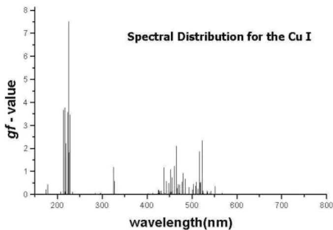
calcula-tion of the odd-parity states. Table 1 shows only the energy parameters for the configurations that are in focus of atten-tion where appear some values for the configuraatten-tion integral which are relevant in the present case. The Fig. 1 shows an illustration of a semi-empirical results for some Cu I lines, where we present a plot of oscillator strengths versus wave-lengths. The figure represents the spectral intensity distribu-tion for copper lines related to the array transidistribu-tions studied here.

Figure 1. Semi-empirical spectrum for the transition of the Cu I.

Brazilian Journal of Physics, vol. 34, no. 4B, December, 2004 1675

Figure 2. Linear plot of equation (1) using Baoming and Hongzhi [5] results for atomic parameters of the Cu I.

Figure 3. Boltzmann plot of equation (1) using semi-empirical gf-values calculated in this work for Cu I spectrum.

4

Conclusions

We hope that the semi-empirical method described in this work can be successfully applied to calculate elec-tron temperature in plasmas. The semi-empirical oscillator strengths calculated by the fitting between theoretical and experimental energy levels produces very good values. This

semi-empirical method produces a very good linear relati-onship betweenln¡

Iλ3_/gf¢

andEu. Its applicability goes

beyond the visible range and may be used in vacuum ultra violet range too. We have made a study of some Cu I lines and determined the plasma temperature of a DC plasma dis-charge that are in acordance with expected. Also, our result is in a very good agreement with the result of Baoming and Hongzhi. The semi-empirical method of measuring tempe-rature gave a difference of 3.5 %.

We present here the oscillator strengths for some known electric dipole transitions in Cu I. The present work is part of an ongoing program, whose goal is to obtain weighted oscil-lator strength,gf, and lifetimes for elements of astrophysical importance. The ions S VII [7], S IX and S X [8], have been concluded.

Acknowledgements

This work was financially supported by the Conse-lho Nacional de Desenvolvimento Cient´ıfico e Tecnol´ogico, CNPq (Brazil), Coordenac¸˜ao de Aperfeic¸oamento de Pes-soal de N´ıvel Superior, CAPES (Brazil), and by Fundac¸˜ao de Amparo `a Pesquisa do Estado do Rio de Janeiro, FAPERJ (Brazil).

References

[1] H. R. Griem,Plasma Spectroscopy, McGraw-Hill: New York (1964).

[2] I. Sobelman, Atomic Spectra and Radiative Transitions. Springer: Berlin (1979).

[3] R. D. Cowan, The Theory of Atomic Structure and Spectra Berkeley, Univ California Press (1981).

[4] L. J. Radziemski and V. Kaufman, J. Opt. Soc. Am.59, 424 (1969).

[5] Baoming Li and Hongzhi Li, 19th International Symposium of Ballistics, 7-11 May 2001, Interlaken, Switzerland.

[6] C. H. Corliss and W. R. Bozman, Experimental Transi-tion Probabilities for Spectral Lines of Seventy Elementes, Washington: National Bureau of Standards Monograph S3, U. S. Government Printing Office (1962).

[7] F. O. Borges, G. H. Cavalcanti, A. G. Trigueiros, and C. Jup´en, J. Quant. Spectrosc. Radiat. Transfer83, 751 (2004).

1676 F. O. Borgeset al.

Table 1: Atomic energy parameters

Configuration Parameter HF Adjusted Adjust/HF

1000cm−1 _1000cm−1

3d104s Eav 0.000 0.000

-3d94s2 Eav 11.580 12.209 1.054

ζ3d 0.810 0.817 1.009

3d104d Eav 45.590 49.942 1.095

ζ4d 0.001 fix

-3d9

4s5s Eav 46.167 64.551 1.398

ζ3d 0.814 0.826 1.015

G2

(3d4s) 9.866 7.828 0.793

G2

(3d5s) 0.711 0.676 0.951

G0

(4s5s) 1.665 0.934 0.561 3d10

4p Eav 27.830 31.752 1.141

ζ4p 0.129 0.183 1.419

3d9

4s4p Eav 28.528 46.553 1.632

ζ3d 0.813 0.663 0.815

ζ4p 0.248 0.203 0.819

F2

(3d4p) 9.289 9.185 0.989

G2

(3d4s) 8.749 8.109 0.927

G1

(3d4p) 3.348 3.103 0.927

G3

(3d4p) 2.619 2.428 0.927

G1

(4s4p) 33.176 20.699 0.624 Integral of Configuration Interaction

3d10

4s-3d9

4s2

R2

d(3d3d,3d4s) -3.744 fix -3d10

4s-3d9

4s5s R2

d(3d3d,3d5s) -0.941 fix -3d10

4s-3d9

4p2

R1

d(3d4s,4p4p) -11.396 fix -3d10

4s-3d9

4p5p R1

d(3d4s,4p5p) -3.344 fix

-R1

e(3d4s,4p5p) -4.126 fix -3d9

4s2

-3d10

4d R2

d(4s4s,3d4d) -1.529 fix -3d9

4s2

-3d9

4s5s R0

d(3d4s,3d5s) 0.235 fix

-R2

e(3d4s,3d5s) 2.341 fix

-R0

d(4s4s,4s5s) 2.189 fix -3d94s2-3d94p2 R1

d(4s4s,4p4p) 36.021 fix -3d94s2-3d94p5p R1

d(4s4s,4p5p) 9.939 fix -3d10

4d-3d9

4s5s R2

d(3d4d,4s5s) 0.861 fix

-R2

e(3d4d,4s5s) -0.215 fix -3d10

4d-3d9

4p2

R1

d(3d4d,4p4p) -2.441 fix

-R3

d(3d4d,4p4p) -1.000 fix -3d10

4d-3d9

4p5p R1

d(3d4d,4p5p) -1.156 fix

-R3

d(3d4d,4p5p) -0.018 fix

-R1

e(3d4d,4p5p) -0.675 fix

-R3

e(3d4d,4p5p) -0.276 fix -3d94s5s-3d94p2 R1

d(4s5s,4p4p) -2.222 fix -3d94s5s-3d94p5p R1

d(4s5s,4p5p) 8.095 fix

-R1

e(4s5s,4p5p) 0.815 fix -3d10

4p-3d9

4s4p R2

d(3d3d,3d4s) -3.715 fix

-R2

d(3d4p,4s4p) -8.208 fix

-R2

e(3d4p,4s4p) -8.398 fix -3d9

4s4p-3d10

5p R2

d(4s4p,3d5p) -3.324 fix

-R1

e(4s4p,3d5p) -3.553 fix

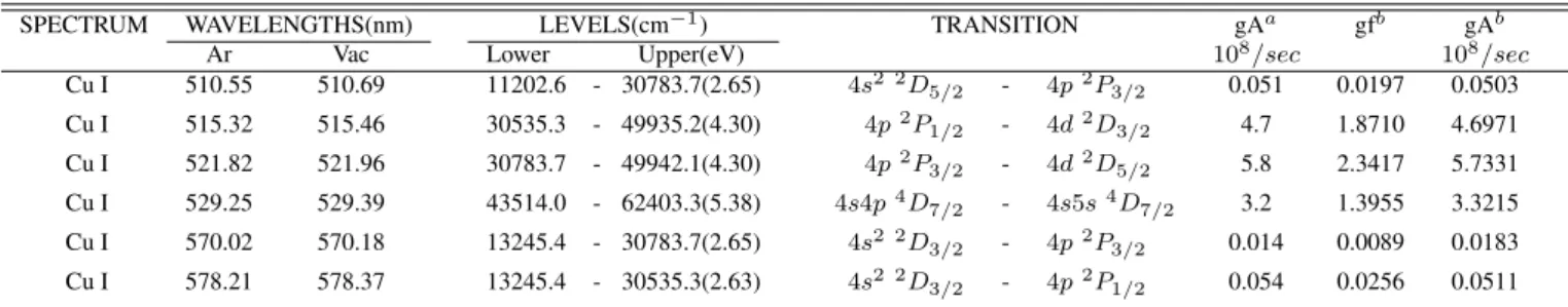
-Table 2: Transition probabilities, oscillator strengths and energy levels for the copper lines

SPECTRUM WAVELENGTHS(nm) LEVELS(cm−1_{) TRANSITION gA}a _gfb _gAb

Ar Vac Lower Upper(eV) 108

/sec 108

/sec

Cu I 510.55 510.69 11202.6 - 30783.7(2.65) 4_s2 2_D5_/2 - 4p 2

P3_/2 0.051 0.0197 0.0503

Cu I 515.32 515.46 30535.3 - 49935.2(4.30) 4_p2

P1_/2 - 4d2D3_/2 4.7 1.8710 4.6971

Cu I 521.82 521.96 30783.7 - 49942.1(4.30) 4_p2

P3_/2 - 4d2D5_/2 5.8 2.3417 5.7331

Cu I 529.25 529.39 43514.0 - 62403.3(5.38) 4_s4_p4

D7/2 - 4s5s 4

D7/2 3.2 1.3955 3.3215

Cu I 570.02 570.18 13245.4 - 30783.7(2.65) 4_s2 2

D3/2 - 4p 2

P3/2 0.014 0.0089 0.0183

Cu I 578.21 578.37 13245.4 - 30535.3(2.63) 4_s2 2

D3/2 - 4p 2

P1/2 0.054 0.0256 0.0511