Lorentz Invariance for Mixed Neutrinos
Massimo Blasone,
Dipartimento di Fisica and INFN, Universit `a di Salerno, 84081 Baronissi (SA), Italy
Jo˜ao Magueijo, and Paulo Pires Pacheco
The Blackett Laboratory, Imperial College London, London SW7 2AZ, U.K.
Received on 23 January, 2005
We show that a proper field theoretical treatment of mixed (Dirac) neutrinos leads to non-trivial dispersion relations for the flavor states. We analyze such a situation in the framework of the non-linear relativity schemes recently proposed by Magueijo and Smolin. We finally examine the experimental implications of our theoretical proposals by considering the spectrum and the end-point of beta decay in tritium.
1
Introduction
The subject of neutrino oscillations has now matured from an insightful prediction by Bruno Pontecorvo [1] and the early results of Homestake [2] to a structured framework backed by a wealth of new quantitative data [3-6]. This advances have been paralleled by much progress on the theoretical front with the efforts divided between phenomenological pursuits of more refined oscillation formulas and attempts to give the theory a sound formal structure within Quantum Field The-ory (QFT).
A major outstanding question was that of the existence of a Hilbert space for the flavour states [7]. The Pontecorvo treatment of the latter in Quantum Mechanics (QM) actually turns out to be forbidden by the Bargmann super-selection rules [8]. This naturally pointed to QFT where the prob-lem found its resolution [9-12]. Subsequently an even more consistent picture emerged with the discovery of an associ-ated geometric phase [13], the extension to the case of three-flavours [14] and bosons [15, 16] and to the case of neutral fields [17]. The study of relativistic flavor currents [18, 19] was recently used to solve the phenomenologically very rele-vant problem of finding a space-oscillation formula [20].
Another important outcome of these studies is the under-standing that the flavour eigenstates constitute the real physi-cal entities, in contrast with the common view where the mass eigenstates are taken to be the fundamental objects [21].
The present paper proceeds in that direction by finding dispersion relations for the mixed neutrinos taking into ac-count their nature as fundamental particles. We find that these dispersion relations no longer have the standard form thus ex-hibiting some form of breakdown of Lorentz invariance. This development is rather timely given the strong interest gener-ated by various schemes involving such modifications [22-27].
We further study the experimental implications of our analysis and compare it with the standard treatment, by
considering the various possibilities which can arise in the end-point of the beta decay of tritium depending on which scenario turns out to be true.
The paper is organized as follows: In section 2 we show how flavor states can be properly defined in QFT. In section 3 we then consider the dispersion relations associated to such states. In section 4 we study the covariance of these forms and the description of the non-linear representation of the Poincar´e algebra necessary to support them. Finally in sec-tion 5 we propose experimental tests, with special emphasis on the end-point of beta decay of tritium. Section 6 is devoted to conclusions.
2
Flavor neutrino states in Quantum
Field Theory
Let us begin our discussion by considering the following Lagrangian density describing two free Dirac fields with a mixed mass term (see Appendix for conventions and further details):
L(x) = ¯Ψf(x) (i6∂−M) Ψf(x), (1)
whereΨT
f = (νe, νµ)andM = µ
me meµ
meµ mµ ¶
. The mix-ing transformations
νe(x) = cosθ ν1(x) + sinθ ν2(x)
νµ(x) = −sinθ ν1(x) + cosθ ν2(x) (2)
withθbeing the mixing angle, diagonalize the quadratic form of Eq.(1) to the Lagrangian for two free Dirac fields, with massesm1andm2:
whereΨT
m = (ν1, ν2)andMd = diag(m1, m2). One also
has me = m1cos2θ +m2sin2θ , mµ = m1sin2θ +
m2cos2θ,m
eµ = (m2−m1) sinθcosθ. Without loss of
generality we takeθranging from0to π4 (maximal mixing) andm2> m1.
The generator for the mixing relations (2) can be intro-duced as [9]:
νσ(x) ≡ G−θ1(t)νj(x)Gθ(t), (4)
Gθ(t) = exp ·
θ
Z
d3x³ν†
1(x)ν2(x)−ν2†(x)ν1(x)
´¸
. (5)
with(σ, j) = (e,1),(µ,2)andt≡x0. Note thatGθ(t)does
not leave invariant the vacuum|0i1,2:
|0(t)ie,µ=G−θ1(t)|0i1,2. (6) We will refer to|0(t)ie,µas to theflavor vacuum: it is
orthog-onal to|0i1,2 in the infinite volume limit [9]. We define the flavor annihilators, relative to the fieldsνe(x)andνµ(x)as
αrk,σ(t) ≡ G−θ1(t)α r
k,jGθ(t) (7)
βr−†k,σ(t) ≡ G−1
θ (t)β r†
−k,jGθ(t) (8)
with(σ, j) = (e,1),(µ,2). The flavor fields can then be ex-panded in analogy to the free field case:
νσ(x) = X
r=1,2
Z d3k
(2π)32
£
ur
k,j(t)αrk,σ(t)
+vr
−k,j(t)β r† −k,σ(t)
i
eik·x.
(9)
with(σ, j) = (e,1),(µ,2).
The symmetry properties of the Lagrangian (1) have been studied in Ref.[18]: one has a total conserved chargeQ as-sociated with the globalU(1)symmetry and time-dependent charges associated to the (broken)SU(2)symmetry. Such charges are the relevant physical quantities for the study of flavor oscillations [10, 14]. They are also essential in the defi-nition of (physical) flavor neutrino states, as the one produced in a beta decay, for example.
In the present case of two flavors, we obtain for the flavor charges [18]:
Qσ(t) = Z
d3xν†
σ(x)νσ(x) (10)
= X
r Z
d3k³αr† k,σ(t)α
r
k,σ(t) −β r† −k,σ(t)β
r
−k,σ(t) ´
,
withσ = e, µ. By indicating with Qj (j = 1,2), the
(con-served) charge operators for the free fields, we obtain the fol-lowing relations:
Qσ(t) =G−θ1(t)QjGθ(t), (σ, j) = (e,1),(µ,2),(11) X
σ
Qσ(t) = X
j
Qj=Q ; [Q, Gθ(t)]6= 0 (12)
Thus the single neutrino and antineutrino states of definite flavor are defined in the following way:
Qσ(t)|νσk(t)i = |ν
k
σ(t)i,
Qσ(t)|ν¯σk(t)i = −|¯ν
k
σ(t)i (13)
and they naturally turn out to be vectors of the flavor Hilbert spaceHe,µ:
|νk
σ(t)i=α r†
k,σ(t)|0(t)ie,µ (14)
|ν¯k
σ(t)i=βkr,σ† (t)|0(t)ie,µ (15)
One can also define the momentum operator for mixed fields [17]:
Pσ(t) = Z
d3xνσ†(x)(−i∇)νσ(x) (16)
=X
r Z
d3k k³αrk†,σ(t)αr
k,σ(t) +β r†
k,σ(t)βkr,σ(t) ´
with
Pσ(t) =G−θ1(t)PjGθ(t), (σ, j) = (e,1),(µ,2),(17) X
σ
Pσ(t) = X
j
Pj =P ; [P, Gθ(t)]6= 0 (18)
wherePj (j = 1,2) are the (conserved) momentum
opera-tors for the free fields andPis the total momentum operator for the system (1), (3). It is immediate to verify that the flavor states Eq.(14),(15) have definite momentum (and helicity):
Pσ(t)|νσk(t)i = k|ν
k
σ(t)i (19)
Pσ(t)|ν¯σk(t)i = k|ν¯
k
σ(t)i. (20)
Note that the above defined flavor states differ from the ones commonly used which are defined by (erroneously) as-suming that the Hilbert spaces for the flavor and the mass fields are the same. For further convenience we denote with a index “P” the Pontecorvo flavor states:
|νeiP = cosθ |ν1i+ sinθ|ν2i
|νµiP = −sinθ|ν1i+ cosθ|ν2i (21)
for which we do not specify the momentum index: as it is well known [28], the flavor states so defined cannot have the same momentum or energy in all inertial frames. Note also that the states (21) are not eigenstates of the momentum and charge operators (defined in Eqs.(13) and (16)) as they are not the vectors of the flavor Hilbert space.
In the following, we will work in the Heisenberg picture, so the Hilbert space is chosen at the reference timet= 0. We thus define our flavor states like
|νk
σi ≡ α r†
k,σ(0)|0(0)ie,µ,
|ν¯k
σi ≡ β r†
3
Dispersion relations for mixed
neu-trinos
Let us now consider the explicit expression for the one electron-neutrino state with definite helicity and momentum (att= 0):
|νk
ei = Y
k G−1
k (θ)α
r†
k,1|0i1,2=
h
cosθ αrk†,1+
+ |Uk| sinθ αrk†,2 −ǫ|Vk|sinθ α
r† k,1α
r† k,2β
r† k,1
i
× × G−1
k,s6=r(θ) Y
p6=k G−1
p (θ)|0i1,2. (23)
where we usedGθ(t) = QkGk(θ). Eq.(23) shows clearly the non-trivial condensate structure of the flavor neutrino states in terms of the mass eigenstates.
Next we consider the energy-momentum tensor. For the massive fieldsνjwe have:
Jjµν(x)≡i νj(x)γν∂µνj(x) , j= 1,2 (24)
from which the Hamiltonians for the free fieldsν1,ν2 triv-ially follow:
Hj=i Z
d3xνj†(x)∂0νj(x)
=X
r Z
d3k³αrk†,j(t)∂0αr
k,j(t) +βkr,j(t)∂0β r† k,j(t)
´
=X
r Z
d3kωk,j ³
αrk†,jαr
k,j−βkr,jβ r† k,j
´
, (25)
with j = 1,2. In a similar way we define the energy-momentum tensor for the flavor fields:
Jµν
σ (x)≡i νσ(x)γν∂µνσ(x) , σ=e, µ. (26)
The energy operators are now: Hσ(t) =i
Z
d3xν†
σ(x)∂0νσ(x) (27)
=X
r Z
d3k³αr†
k,σ(t)∂0α r
k,σ(t) +βkr,σ(t)∂0β r† k,σ(t)
´
withσ=e, µ. We also easily recover the momentum opera-tors (16). Notice that Eq.(27) cannot be further reduced as for Eq.(25), due to the non-trivial time dependence of the flavor ladder operators.
In conclusion we find:
Hσ(t)6=G−θ1(t)HjGθ(t), (σ, j) = (e,1),(µ,2).(28) X
σ
Hσ(t) = X
j
Hj=H ; [H, Gθ(t)]6= 0 (29)
The inequality sign in (28) can be understood by noting the appearance of the time derivative in the definition (27) and the fact that the mixing generator is time dependent. Con-sequently, the result (29) is non-trivial and ensure the fact
that the expectation value of the total (flavor field) energy on states in the flavor Hilbert space is time-independent.
We indeed have:
e,µh0|H|0ie,µ = − Z
d3k(ωk,1+ωk,2)× ×(1 −2 sin2θ|Vk|2) (30)
This has to be compared with the mass vacuum zero point energy:
1,2h0|H|0i1,2 = −
Z
d3k(ωk,1+ωk,2) (31) The flavor vacuum zero-point energy has been studied in Ref.[29] in connection with the cosmological constant.
Of course, both contributions Eqs.(30), (31) are divergent and to properly define energy for flavor states, we need to nor-mal order the Hamiltonian with respect to the relevant vac-uum, namely the flavor vacuum:
::H ::≡ H − e,µh0|H|0ie,µ (32)
where the new symbol for the normal ordering was intro-duced to remember that it refers to the flavor vacuum.
We finally obtain:
Ee(k) ≡ hνek|::H ::|νeki
= ωk,1cos2θ + (1−2|Vk|2)ωk,2sin2θ(33) Eµ(k) ≡ hνµk|::H ::|ν
k
µi
= ωk,2cos2θ + (1−2|Vk|2)ωk,1sin2θ(34) We propose to treat these as modified dispersion relations and to find the corresponding non-linear realization of the Lorentz algebra as outlined in [25]. Obviously the energies in Eqs.(33),(34) are only expectation values subject to fluctu-ations but it is nevertheless sensible to consider the modified Lorentz transformation for these dispersion relations which form the classical limit of the theory.
Note the presence in the above dispersion relations, of the Bogoliubov coefficient|Vk|2: this term is due to the fla-vor vacuum structure and is absent in the usual Pontecorvo case. The maximum of the function|Vk|2occurs fork
max=
√m1m2; we then have:
|Vkmax|
2= 1
2−
1
q
(1 +m1
m2)(1 +
m2
m1)
(35)
If we put a = m1
m2 < 1, then the condition |Vk| 2 ≪ 1
2 is realized for
1> a > b
2−1 + 2b(1−√2b−1)
4
Lorentz invariance for mixed
neutri-nos
In this section, we study the dispersion relations (33), (34) and derive the corresponding non-linear realization of the Lorentz algebra.
First, from Eqs.(33), (34), let us define the rest masses for the mixed neutrinos:
me ≡ Ee(k= 0) = m1cos2θ+m2sin2θ (37)
mµ ≡ Eµ(k= 0) = m2cos2θ+m1sin2θ (38)
Then we investigate the highklimit of Eqs.(33),(34). To first order inm
2
j
2k, it isωk,j ≃k+ m2
j
2k and|Vk|
2≃(m2−m1) 2 4k2 and we obtain:
Ee(k)≃k+ e
m2
e
2k ; me 2
e≡m
2
1cos(2θ) +m1m2sin2θ
Eµ(k)≃k+ e
m2
µ
2k ; me 2
µ≡m22cos(2θ) +m1m2sin2θ where we introduced the effective massesmeeandmeµ. We
thus see that in the high momentum (or equivalently highE since it is a monotonously growing function ofk) limit, the dispersion relations for the flavor neutrinos are indeed of the usual form, although with a modified mass.
Noticing thatωk,1(1−2|Vk|2) = k 2
+m1m2
ωk,2 andωk,2(1−
2|Vk|2) = k2 +m1m2
ωk,1 , we rewrite Eqs.(33), (34) as Ee(k) =
2k2+m1(m2+m1)−m1(m2−m1) cos(2θ)
2pk2+m2 1
(39)
Eµ(k) =
2k2+m2(m2+m1) +m2(m2−m1) cos(2θ)
2pk2+m2 2
(40) By introducinga≡m2/m1≥1, we get
Ee(k) =
k2+m2
1−(1−a)m21sin2θ
p
k2+m2 1
(41)
Eµ(k) =
k2+a2m2
1+a(1−a)m21sin2θ
p
k2+a2m2 1
(42)
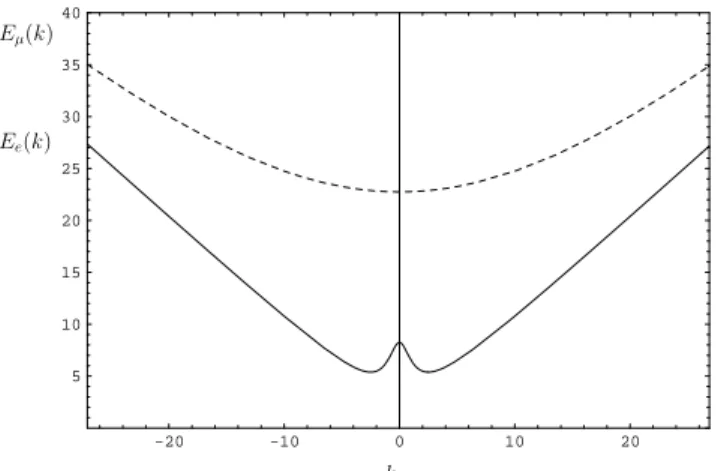
It is easy to realize that, fora >1, the functionEµ(k)has
an absolute minimum atk= 0with the valueEµ(0) =mµ.
The situation is different forEe(k): the minimum is now
atkmin = √12 p
a−3 + (1−a) cos(2θ). This is different from zero whenais above the critical valueac = cos(2cos(2θθ))−−31.
For1 < a < ac, the functionEe(k)has an absolute
mini-mum atk= 0with the valueEe(0) =me.
This is represented in the two figures below for the case θ=π/6⇔ac = 5.
-4 -2 0 2 4
1 2 3 4 5
Eµ(k)
Ee(k)
k
Figure 1.Ee(solid line) andEµ(dashed line) as functions ofkfor
θ=π/6,m1 = 1,a= 2,a c= 5.
-20 -10 0 10 20
5 10 15 20 25 30 35 40
Eµ(k)
Ee(k)
k
Figure 2.Ee(solid line) andEµ(dashed line) as functions ofkfor
θ=π/6,m1 = 1,a= 30,a c= 5.
In the following we consider only the subcritical case a < ac. The casea > acwill be treated elsewhere.
Following Ref.[25], we now set the dispersion relations in the following form:
Ee2fe2(Ee) −k2g2e(Ee) = m2e (43)
Eµ2fµ2(Eµ) − k2gµ2(Eµ) = m2µ (44)
It is now possible to identify the non-linear realization of the Lorentz group which leaves these dispersion rela-tions invariant. They are generated by the transformation U◦(E,k) = (Ef,kg)applied to the standard Lorentz gen-erators (Lab=pa∂p∂b −pb∂p∂a):
Ki=U−1[p0]L0iU[p0]. (45) This amounts to requiring linearity for the auxiliary variables
˜
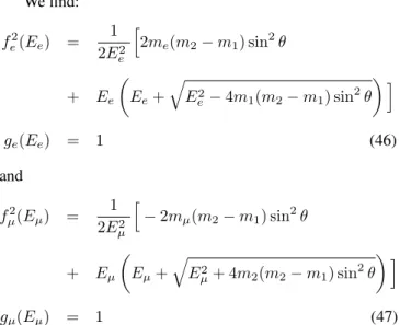
We find: f2
e(Ee) =
1 2E2
e h
2me(m2−m1) sin2θ
+ Ee µ
Ee+ q
E2
e−4m1(m2−m1) sin2θ ¶ i
ge(Ee) = 1 (46)
and
fµ2(Eµ) =
1 2E2
µ h
−2mµ(m2−m1) sin2θ
+ Eµ µ
Eµ+ q
E2
µ+ 4m2(m2−m1) sin2θ ¶ i
gµ(Eµ) = 1 (47)
It is easy to check that, form1 =m2and/orθ= 0, we have f2
e(Ee) =fµ2(Eµ) = 1. Alsofµ2(mµ) = 1(for anya ≥1)
andf2
e(me) = 1(only forac≥a≥1)
A plot of these two functions is given below:
2 4 6 8 10
1.02 1.04 1.06 1.08 1.1
Figure 3.feas a function ofEe(solid line) andfµas a function of
Eµ(dashed line) forθ=π/6,m1= 1,a= 4,ac= 5.
For large values ofEeandEµ,fe2(Ee)andfµ2(Eµ)can
be approximated as:
fe2(Ee) ≃ 1 −
1
E2
e
(m2−m1)2sin4θ (48)
fµ2(Eµ) ≃ 1 −
1
E2
µ
(m2−m1)2sin4θ (49)
showing that the Lorentzian regime is approached quadrati-cally as the energy (momentum) grows.
5
Phenomenological consequences
We now focus on some phenomenological consequences which arise from considering the flavor states as fundamental and consequently the non-standard dispersion relations (33), (34) as characterizing mixed neutrinos.
We consider the case of a beta decay process like tri-tium decay, which allows for a direct investigation of neu-trino mass. In the following we take into account the various possible outcomes of this experiment in correspondence of the different theoretical possibilities for the nature of mixed neutrinos. We show that significative differences arise at phe-nomenological level between the standard theory and the sce-nario above described.
Let us then consider the decay: A→B+e−+ ¯ν
e
whereAandBare two nuclei (e.g.3H and3He).
The electron spectrum is proportional to phase volume factorEpEepe:
dN
dK =CEp(Q−K)
p
(Q−K)2 −m2
e (50)
whereE = m+K andp =√E2−m2are electron’s en-ergy and momentum. We denote by methe electron
(anti-)neutrino mass.
The endpoint ofβ decay is the maximal kinetic energy Kmaxthe electron can take (constrained by the available
en-ergyQ=EA−EB−m≈mA−mB−m). In the case of
tritium decay,Q= 18.6KeV.Qis shared between the (un-measured) neutrino energy and the ((un-measured) electron ki-netic energyK.
It is clear that if the neutrino were massless, thenme= 0
andKmax=Q.
On the other hand, if the neutrino were a mass eigenstate (say withme=m1), thenKmax=Q−m1.
We now consider the various possibilities which can arise in the presence of mixing:
•If, following the common wisdom, mass eigenstates are considered fundamental, theβ spectrum is
dN
dK =CEp Ee
X
j
|Uej|2 q
E2
e−m2j Θ(Ee−mj) (51)
whereEe=Q−KandUej= (cosθ,sinθ)andΘ(Ee−mj)
is the Heaviside step function.
The end point is atK=Q−m1and the spectrum has an inflexion atK≃Q−m2.
If flavor neutrinos are to be taken as fundamental, we have the following two options:
• Assuming that nuclei and the electron satisfy linear Lorentz transformations, and that Eefe(Ee)transforms
lin-early, the only covariant law of energy conservation is EA=EB+E+Eefe(Ee).
The endpoint ofβ decay is nowKmax = Q−meand
the β spectrum is proportional to the phase volume factor EpEefe(Ee)pe:
dN
dK =CEp(Q−K)
p
(Q−K)2−m2
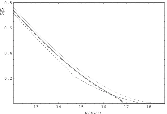
13 14 15 16 17 18 0.2
0.4 0.6 0.8
dN dK
K(K eV)
Figure 4. The tail of the tritiumβspectrum for: - a massless neutrino (dotted line); - a Lorentz invariant flavor state (solid line); - preferred frame (long-dashed line); - superposed prediction for 2 mass states (short-dashed line): notice the inflexion in the spectrum where the most massive state switches off. We usedme= 1.75KeV,m1 = 1KeV,m2= 4KeV,θ=π/6.
• If, on the contrary, we insist upon the standard law EA=EB+E+Ee
we have introduced a preferred frame, and are in conflict with the principle of relativity.
ThenKmax=Q−meand the spectrum is proportional
to the phase volume factorEpEepe:
dN
dK =CEp(Q−K)
p
(Q−K)2f2
e −m2eΘ(Ee−me)
(53) The above possibilities are plotted in Fig.(), together with the spectrum for a massless neutrino, for comparison.
We note that the next generation tritium beta decay exper-iments will allow a sub-eV sensitivity for the electron neu-trino mass [31], thus hopefully allowing to unveil the true nature of mixed neutrinos.
6
Conclusions
In this paper, we have investigated some aspects of neutrino mixing in Quantum Field Theory. From a careful analysis of the Hilbert space structure for flavor (mixed) fields it has emerged that the flavor states, defined as eigenstates of the flavor charge, are at odds with Lorentz invariance. Indeed they exhibit non-standard dispersion relations, which how-ever reduce to the usual (Lorentzian) ones in the relativistic limit.
We have then shown that it is possible to account for such a modified dispersion relations, by resorting to a recent pro-posal [25]: According to this, we could identify a non-linear
representation of the Lorentz group allowing for these disper-sion relations and ensuring at the same time the equivalence of inertial observers.
Finally, we have considered possible phenomenological consequences which can arise from our analysis, by looking at the beta decay. We have considered various possibilities, including that of introducing a preferred frame, and shown that observable differences arise in correspondence of the var-ious cases.
Acknowledgments
M. B. acknowledges partial support from MURST, INFN, INFM and ESF Program COSLAB. P. P. P. thanks the FCT (part of the Portuguese Ministry of Education) for financial support under scholarship SFRH/BD/10889/2002.
Appendix A: Flavor Hilbert space
The free fieldsν1(x)andν2(x)are written as
νj(x) = X
r=1,2
Z d3k
(2π)32
eik·x£ur
k,j(t)αrk,j
+vr−k,j(t)β r† −k,j
i
, j= 1,2. (54)
Hereur
k,j(t) =e−iωk,jturk,j andvkr,j(t) = eiωk,jtvrk,j, with
ωk,j = q
|k|2+m2
The orthonormality and completeness relations are: urk†,jus
k,j =v r† k,jv
s
k,j =δrs,
urk†,jv s
−k,j =v r† −k,ju
s
k,j = 0, X
r
(ur
k,ju r† k,j+v
r
−k,jv r†
−k,j) = 1I2. (55)
where1Inis then×nunit matrix.
The αr
k,j and the βrk,j, j, r = 1,2 are the
annihila-tion operators for the vacuum state |0i1,2 ≡ |0i1 ⊗ |0i2: αr
k,j|0i12=βkr,j|0i12= 0.
The anticommutation relations are: {να
i(x), ν β†
j (y)}t=t′ = δ3(x−y)δαβδij, α, β= 1, ..,4,
{αr
k,i, αsq†,j}=δ
3(k
−p)δrsδij,
{βkr,i, β s† q,j}=δ
3(k
−q)δrsδij, i, j= 1,2. (56)
All other anticommutators are zero.
In the reference frame where k is collinear with kˆ ≡
(0,0,1), the flavor annihilation operators have the simple form:
αr
k,e(t) = cosθ αrk,1 + sinθ
¡
U∗ k(t)αrk,2
+ǫr
kVk(t)β
r† −k,2
´
(57) αrk,µ(t) = cosθ αrk,2 − sinθ
¡
Uk(t)αrk,1
−ǫrkVk(t)β
r† −k,1
´
(58) βr
−k,e(t) = cosθ βr−k,1 + sinθ
¡
U∗
k(t)β−rk,2 −ǫrkVk(t)α
r† k,2
´
(59) βr
−k,µ(t) = cosθ βr−k,2 − sinθ
¡
Uk(t)βr
−k,1
+ǫr
kVk(t)α
r† k,1
´
(60) whereǫr
k ≡ (−1)r+k· ˆ
k+1 andUk(t),Vk(t)are Bogoliubov coefficients given by:
Uk(t) ≡ urk†,2(t)ur
k,1(t) =vr−†k,1(t)vr−k,2(t)
= |Uk|ei(ωk,2−ωk,1)t ,
Vk(t) ≡ ǫr
ku
r†
k,1(t)vr−k,2(t) =−ǫrku
r†
k,2(t)vr−k,1(t)
= |Vk|ei(ωk,2+ωk,1)t
(61) with
|Uk|= |k|
2+ (ω
k,1+m1)(ωk,2+m2)
2pωk,1ωk,2(ωk,1+m1)(ωk,2+m2) ,
|Vk|= (ωk,1+m1)−(ωk,2+m2) 2pωk,1ωk,2(ωk,1+m1)(ωk,2+m2)
|k|,
|Uk|2+|Vk|2= 1. (62)
References
[1] B. Pontecorvo, Zh. Eksp. Theor. Fiz.33, 549 (1958); Sov. Phys. JEPT 6, 429 (1958); Z. Maki, M. Nakagawa, and
S. Sakata, Prog. Theor. Phys.28, 870 (1962); V. Gribov and B. Pontecorvo, Phys. Lett. B28, 493 (1969); S. M. Bilenky and B. Pontecorvo, Phys. Rep.41, 225 (1978).
[2] J. Davis, D. S. Harmer, and K. C. Hoffmann, Phys. Rev. Lett.
20, 1205 (1968).
[3] M. Koshiba, in: *Erice 1998, From the Planck length to the Hubble radius* 170; S. Fukuda et al. (Super-Kamiokande col-laboration), Phys. Rev. Lett.86, 5656 (2001).
[4] Q. R. Ahmad et al. (SNO collaboration) Phys. Rev. Lett.87, 071301 (2001); Phys. Rev. Lett.89, 011301 (2002).
[5] K. Eguchiet al.(KamLAND Collaboration), Phys. Rev. Lett.
90, 021802 (2003).
[6] M. H. Ahn et al. (K2K Collaboration), [hep-ex/0212007].
[7] T. Kaneko, Y. Ohnuki, and K. Watanabe, Prog. Theor. Phys.
30, 521 (1963); K. Fujii, Nuovo Cimento34, 722 (1964).
[8] V. Bargmann, Annals Math. 59, 1 (1954); A. Galindo and P. Pascual, Quantum Mechanics, (Springer Verlag, Berlin, 1990).
See also: D. M. Greenberger, Phys. Rev. Lett.87, 100405 (2001).
[9] M. Blasone and G. Vitiello, Annals Phys.244, 283 (1995); Er-ratum: ibid.249, 363 (1995).
[10] M. Blasone, P. A. Henning, and G. Vitiello, Phys. Lett. B451, 140 (1999); M. Blasone, in: *Erice 1998, From the Planck length to the Hubble radius* 584-593; M. Blasone and G. Vi-tiello, Phys. Rev. D60, 111302 (1999).
[11] K. C. Hannabuss and D. C. Latimer, J. Phys. A 33, 1369 (2000); J. Phys. A36, L69 (2003).
[12] K. Fujii, C. Hab, and T. Yabuki, Phys. Rev. D 59, 113003 (1999); Erratum: ibid. D60, 099903 (1999); Phys. Rev. D
64, 013011 (2001); K. Fujii, C. Habe, and M. Blasone, [hep-ph/0212076].
[13] M. Blasone, P. A. Henning, and G. Vitiello, Phys. Lett. B466, 262 (1999); X. B. Wang, L. C. Kwek, Y. Liu, and C. H. Oh, Phys. Rev. D63, 053003 (2001).
[14] M. Blasone, A. Capolupo and G. Vitiello, Phys. Rev. D66, 025033 (2002).
[15] M. Blasone, A. Capolupo, O. Romei, and G. Vitiello, Phys. Rev. D63, 125015 (2001); M. Blasone, P. A. Henning, and G. Vitiello, in: “La Thuile 1996, Results and perspectives in particle physics” 139-152.
[16] M. Binger and C. R. Ji, Phys. Rev. D 60, 056005 (1999); C. R. Ji and Y. Mishchenko, Phys. Rev. D64, 076004 (2001); Phys. Rev. D65, 096015 (2002).
[17] M. Blasone and J. Palmer, Phys. Rev. D69, 057301 (2004).
[18] M. Blasone, P. Jizba, and G. Vitiello, Phys. Lett. B517, 471 (2001).
[19] M. Blasone, P. P. Pacheco, and H. W. Tseung, Phys. Rev. D67, 073011 (2003).
[20] M. Beuthe, Phys. Rev. D66, 013003 (2002); Phys. Rep.375, 105 (2003).
[21] C. Giunti, [hep-ph/0409230].
[23] A. Albrecht and J. Magueijo, Phys. Rev. D59, 043516 (1999).
[24] S. Alexander and J. Magueijo, [hep-th/0104093].
[25] J. Magueijo and L. Smolin, Phys. Rev. D67, 044017 (2003); Phys. Rev. Lett.88, 190403 (2002).
[26] D. Kimberly, J. Magueijo and J. Medeiros, Phys. Rev. D70, 084007 (2004).
[27] G. Amelino-Camelia, Int. J. Mod. Phys. D11, 35 (2002).
[28] C. Giunti, Mod. Phys. Lett. A16, 2363 (2001).
[29] M. Blasone, A. Capolupo, S. Capozziello, S. Carloni, and G. Vitiello, Phys. Lett. A323, 182 (2004); [hep-th/0412165].
[30] M. Blasone, J. Magueijo, and P. Pires-Pacheco, [hep-ph/0307205].