College entry exams: A dynamic discrete choice model
Jose Raimundo Carvalho and Thierry Magnac
yFirst version: July 2009
This version: April 30, 2010
Comments welcome
Abstract
A simple mechanism is used in some universities in Brazil to select students at entry and allocate them into various majors. Students …rst choose a major and then take exams that either select them in the chosen major or select them out. The matching literature analyzing the student placement issue, points out that this mechanism is not fair and is strategic. Pairs of major & students can be made better o¤ and students tend to disguise their preferences. We build up a dynamic model of choice of major and of grading as well as e¤ort exerted to be successful where preferences are carefully modelled. We estimate this model by simulated maximum likelihood using cross-section data about entry exams at Universidade Federal do Ceara in Brazil in 2004. Using the empirical results of the model estimation, we then evaluate changes in the way choices are given to the prospective students. Ex-ante expected utilitarian social welfare indeed increases but it hides very strong distributive e¤ects among students. Strategic e¤ects are found to be very strong.
CAEN, Universidade Federal do Ceara, Fortaleza, Brazil.
1
Introduction
1University access in Brazil is a very competitive process and even …ercer if one restricts the analysis to public universities, on average the best institutions: More than two millions of students competed to access one of the 331,105 seats in 2006. For some majors, in Medicine or Law for instance, the ratio of students to available seats can be as high as 20 or more (INEP, 2008). Fierce competition is by no means an exclusivity of the process of entrance into Brazilian universities as many developed and developing countries are in a similar situation (Manski and Wise, 1983). What makes Brazil speci…c is the formality of the selection process. In contrast to countries such as the United States where the predominant selection system uses multiple criteria (for instance, Arcidiacono, 2005), selection through exams and objective grading only is pervasive in Brazil. More than 88% of available seats are allocated through avestibular as is called the sequence of exams taken by applicants to university degrees (INEP, 2008).
In this paper, we use comprehensive data on the choices of majors by students and the grades that they obtain at the vestibular of the Universidade Federal do Ceará (UFC thereafter) in Northeast Brazil in 2004 and we concentrate on the speci…cs of this case. The main characteristics of that speci…c vestibular is that the student chooses a single undergraduate major before the exams and competes against those students who made the same choice only. Another interesting characteristics is that the exam consists in two stages. The …rst stage is common to all majors and is comprised of many sub-exams, each one evaluating knowledge in a de…nite subject, i.e. Mathematics, Portuguese etc.. The second stage is speci…c to each major and comprises two sub-exams.
What should be the optimal organization of the vestibular? This is known in the literature in economics as the college admission problem. This subject has a long history and a brief survey of the recent literature on one of the most popular solution is given in Roth (2008). The issue at hand is to match students with colleges which are in our case, the schools o¤ering undergraduate majors at the university (medicine, engineering and so on). In the case where college preferences are simple2 and consist in attracting the students who are the best in their discipline, it boils down to what is called student placement (Balinski and Sönmez, 1999) or one-sided matching. The 1We thank CNRS and CNPq for funding (Project 21207). Comments by participants at conferences in Brown, Bristol and Atlanta and seminars in Oxford and CREST, Paris are gratefully acknowledged. The usual disclaimer applies.
matching mechanisms that are studied are supposed to satisfy certain properties. First, they could be stable, or fair in the student placement literature, in the sense that there is no pair (student, college) who would like to block the …nal allocation in order to improve their lot by matching with another partner. Second, the mechanisms could be strategy proof i.e. every student has an interest to reveal her true preferences. Stable mechanisms are not unique and some of them are better for the students and others are better for the schools.
Among those mechanisms, the Gale Shapley student optimal stable mechanism (hereafter GS mechanism) satis…es the properties of stability and strategy-proofness and is optimal among those mechanisms from the student perspective (Abdulkadiroglu and Sonmez, 2003). In the GS mecha-nism, the …rst step consists in each student proposing to her preferred school. Each school tentatively ranks all its proposers (with respect to the possibly speci…c preference ranking the school has or using a lottery to break ties) and rejects the ones in surplus with respect to the number of seats the school has and which is …xed and publicly known ex-ante. In further steps of the algorithm, every student who was rejected in the previous steps proposes to her next choice. Each school ranks all its proposers (the ones from the previous step AND the new ones) and rejects the ones in surplus with respect to the number of seats. A student who was not rejected in the …rst step can well be rejected in further steps. This algorithm, also called a deferred acceptance algorithm, terminates when all new student proposals are rejected and nothing can be modi…ed.
We can then compare the vestibular at UFC to the Gale Shapley mechanism. As a matter of fact it turns out that the vestibular at UFC corresponds to step 1 only of the GS algorithm. Students are allowed to propose to their …rst choice only. This is why the mechanism loses its two properties: it is not stable (i.e. there exist pairs of student & school which could be made better o¤ by changing the …nal allocation) and it is not strategy proof. Some students prefer to disguise their preferences for very demanded disciplines (medicine, law,. . . ) in order to improve their probability of being accepted. The present form under which the vestibular is organized at UFC is thus di¢cult to justify.
mechanism is known to be not stable and actors play strategically and disguise their preferences. This recent research questions that the Gale Shapley mechanism leads to a Pareto solution in terms of ex-ante utilities (Abdulkadiro¼glu, Che and Yasuda, 2008 in a school choice problem, Budish and Cantillon, 2010 in a multi-unit assignment problem). Those papers exhibit other mechanisms that are not stable and not strategyproof although they are dominating the GS mechanism in terms of ex-ante utility. the main intuition for this result is that the latter mechanism does not allow applicants to reveal the intensity of their preferences, just the ranking of them.
What we do in this paper is to contribute to teh empirical literature on this subject by evaluating thisvestibular using some counterfactual mechanisms. We start by constructing a dynamic model of choice of majors following the literature about choices of colleges (Arcidiacono, 2006 and Bourdabat and Montmarquette, 2007, for instance). In contrast to this literature though, we cannot use information on wages after school and we model them as undistinguishable from preferences. Choice probabilities of majors thus depend on (1) expected probabilities of success and (2) preferences for the majors.
In addition, we shall consider that exams have both a dimension of selection of the most tal-ented (although the selection is imperfect) but also of those who exert more e¤ort. The tournament literature indeed insists on the double dimension of selection and incentives that exams, or tour-naments, have and distinguishing between them is one of the substantive issues studied in applied research (Davies and Stoian, 2007 or Leuven, Osterbeek, Sonnemans and van der Klaauw, 2008). It is also interesting to include e¤ort since it allows students to reveal the degree of preferences that they have for di¤erent majors since higher preferences lead to higher e¤ort and thus increases their probabilities of success.
The advantage of these data is that we can carefully model the probability of success at entry of each school using data on performances that we have i.e. the grades at the two stages of the exam as well as an initial measure of talent obtained a year before the exam is taken. We adopt the assumption that expectations are perfect (see Manski, 1992, for a critical evaluation of this assumption) and thus that players are sophisticated. The thresholds above which students are accepted into the programs are the results of the Nash equilibrium of this game in which beliefs are given by what is observed in the data and in which each player is assumed to be small.
by UFC that we restrict, for simplicity, to the choice process into three majors in medicine, the most competitive major …eld. We use parametric models for the success probabilities and prefer-ences although we study non parametric identi…cation of the model. Using these empirical results, we then construct counterfactuals by recomputing the Nash equilibrium under the counterfactual mechanism. Speci…cally, we analyze the mechanism which allows students to have two choices in-stead of one and thus play less strategically. We show that indeed, enlarging the choice set has a positive aggregate e¤ect in terms of utilitarist social welfare but has also strong distributive e¤ects. The strategic e¤ects are shown to be very important.
This paper builds upon various literatures and in particular student placement. There are a few papers concerned by the analysis of school choice (Lai, Sadoulet and de Janvry, 2009) and the Boston mechanisms using Chinese data (He, 2009) or the GS mechanism using US data (Abdulkadiro¼glu, Pathak and Roth, 2009). In a more theoretical work but oriented towards the analysis of a speci…c mechanism, Balinski and Sönmez (1999) study the optimality of the placement of students in Turkish universities although the selection there concerns all students & colleges throughout the country. Students …rst write exams in various disciplines and scores are constructed by each college. Colleges choose the weight that they give to di¤erent …elds: grades in maths can presumably be given more weight by math colleges. They show that this mechanism is suboptimal with respect to the Gale & Shapley mechanism.
Section 2 describes the set-up and the game that applicants play. The identi…cation and esti-mation of the econometric model is the object of Section 3. Section 4 reports the empirical analysis and counterfactual scenarii are studied in Section 5. Section 6 concludes.
2
Description & modelling
having a rank above a multiple (usually 4 sometimes 3) of the number of available positions in the chosen major. This ranking procedure at the …rst stage as well as at the second stage de…nes thresholds in terms of grades that determine if the exam is passed. Appendix B gives further details on the exam.
We consider a parsimonious theoretical set-up building up from models of college choices and of tournaments. Students are supposed to be heterogenous in talent a single dimensional term and students have preferences over di¤erent majors which can be monetary or non monetary. The former include rewards that a degree in a speci…c major raises in the labor market. Furthermore, we consider that entry is not a matter of talent and preferences alone but depends also on a variable called e¤ort exerted before the exams. Talent and e¤ort are distinguished so that both selection and incentives are the two main operating determinants of success in tournaments.
We analyze the entry exams as a game between students in which information is incomplete. Agents do not know the types of competing students, only their distribution in the population. They do know however their own talent and their own preferences. We shall consider Nash equilibria of this game for all students. We thus write the decision model for any student where we consider that actions, or choice probabilities, taken by any other student and which are described below are …xed.
In dynamic models, assumptions about expectations play a key rôle (Manski, 1992). We assume that expectations about own grades and others’ grades, which are uncertain, are perfect, in the sense that the distribution of those random variables are equal to the distribution of those in the data. Even if there are multiple equilibria of the game, a point we shall return to in the section about counterfactuals, we nevertheless assume that everybody coordinates on the equilibrium that is observed in the data. Therefore, all thresholds determining at which grades the two-stage exams are passed are supposed to be perfectly anticipated. In other words, players are sophisticated. The validity of this assumption is questionned by Lai, Sadoulet & de Janvry (2009) and He (2009).
2.1
Timing
We begin with setting up the notations and we omit the individual index for simplicity. Variable
d is a speci…c major and D is the number of such majors. The outside option is denoted d = 0. Observed characteristics of the student are denoted z; an unobserved single dimensional variable,
"; stands for student’s talent and various unobserved tastes for every major are piled up in a vector of preferences u=fudgd=0;:;D. Because preferences are written as a reduced form of future rewards
on the labor market yielded by a speci…c major degree, they are likely to be correlated with talent
".
Step 1: Information: A standardized national exam whose nickname is ENEM is organized
about a year before the entry exam. Denote,m0, the grade obtained at this exam and assume
that:
m0 ="+ 0;
where 0 is a noise scrambling the signal for talent". Talent" is known by each agent ex-ante while 0 is not. The distribution of both is common knowledge among students.
Step 2: Decisions: The student simultaneously chooses one single major, d 2 f0; :; Dg and
resources, y, to apply in terms of hours or expenditures in order to prepare the entry exam into the university. These resources or e¤ort,y, are written in terms of units of higher grades that they allow the student to obtain at least in expectation. We assume that resources y
that are unobserved are written in the same units as talent " is so what impacts the grades is the sum of talent" and resourcesy. Cost of resources is supposed to be quadratic in e¤ort and equal to:
c0(y+cy2=2):
Parameter c0 could be heterogenous across agents and potentially correlated with" although
we will show that its distribution is not identi…ed. On the other hand, parametercis assumed to depend on characteristics z or talent " via a deterministic function only.
Step 3: Information: At the …rst stage of the vestibular, which is common to all majors, the
student gets a grade denoted m1 that we assume is given by:
where 1 is some noise. Students are ranked according to a known weighted combination of grades m0 and m1 decided by the University. The …rst stage is passed and the student
proceeds to Step 2 if and only if the rank of the student among its fellow students in major
d 2 f1; :; Dg is larger than a certain reference rank. We neglect ties that are broken using a formal institutional rule that has marginal importance here. The number of students who are allowed in is equal to three or four times the number of seats available in that major. As m0
is observed by everybody and as we are looking at Nash equilibria, the passing rule can be written as:
m1 t1(d; m0):
Otherwise the exam is failed and the student gets the utility u0 of the outside option. this
is the utility of the best option among; The expected value of investing an additional year so as to try to enter again into the university; The expected value of trying to enter another university, a private or a State university – since both exist in the same town – or in another town; To any other option that the student has, for instance if the student desists once and for all. It is likely that the outside option depends on talent ". Nevertheless, we suppose for simplicity that the value of the outside option does not depend on resourcesyexpended in the last period. The impact of resources y are supposed to be speci…c to the exam taking place this year and at this university. this assumption enables us to argue later on that modifying the selection mechanism does not a¤ect the population of students willing to take the exam.
Step 4: Information: At the second stage,4 the student gets another grade,m
2 and we assume
that:
m2 ="+y+ 2;
where 2is some noise. Again, students are ranked according to a known weighted combination of m0; m1 andm2 and only the higher ranked fraction of students is accepted. Again, we can
write the passing rule as a function of observed grades m0 and m1:
m2 t2(d; m0; m1):
Otherwise, if the grade is smaller than the threshold, the exam is failed and the student gets the outside option u0: Namely, the access to the second stage does not grant any privilege
given unobserved talent and e¤ort. Finally, in case of success, the student gains ud as a
function of future wages, major choice and tastes. We chose this speci…cation because we have no information on wages. Note that ud and talent " are generally correlated through
unobserved wages.
2.2
Observations, Measurements and Expectations
Measurement of talent As a summary, the grades obtained at the di¤erent stages are
func-tions of unobserved talent " and e¤ort y such that: 8
< :
m0 ="+ 0
m1 ="+y+ 1
m2 ="+y+ 2
where i are noises a¤ecting grades. Note that talent and e¤ort have the same e¤ect at the two stages of the exam something that we could try to generalize by using information coming from di¤erent exams (i.e. mathematics, portuguese etc) although it is crucial in this set-up since it allows the identi…cation of the distribution of e¤ort under conditions that we study below.
Expectations The student knows her own talent";tastes & rewardsudand continuation value
u0 and learns about ( 0; 1; 2) at every step. We …rst assume that measurement errors ( 0; 1; 2)
are independently distributed and are independent of any other variables. Their distribution is common knowledge. Furthermore, the student is supposed to know the distribution of the structural random errors (";fudgd=0;:;D) and of covariates z in the population:
Pr(";fudgd=0;:;D jz);
but not the precise shocks a¤ecting competitors. We assume that the anticipated distribution is equal to the actual distribution of these variables in the data. 5
2.3
Solving the model backward
We now write the dynamic model of choice. We do not use a discount factor even if this process takes time, as the discount factor is generically not identi…ed in these dynamic discrete choice models (e.g. Magnac and Thesmar, 2004). We solve the model backward given the information that is available to the agent at each stage.
At Step 4 which is reached in the case of success at the …rst stage exam,m1 > t1(d; m0), the agent
has no decision to take and the history that she conditions on is h1 = ("; m0; y; d; m1) comprising
talent, ", initial and …rst-stage grades,m0 and m1;e¤orty and selected majord. The value of such
an history is the sum of what can be obtained in case of either success or failure:
V2(h1) = Pr
2f
m2 > t2(d; m0; m1)jh1g:ud+ Pr 2f
m2 < t2(d; m0; m1)jh1g:u0:
Given that measurement shocks j are independent, the only thing that matters inh1 are variables
("; y; t2(d; m0; m1) t2d). Thus:
V2("; y; t2d) = Prf 2 > t2d " yg:ud+ Prf 2 t2d " yg:u0:
At the previous step, Step 3, the …rst stage grade is revealed so that the student gains the value
V2(:) if she passes, i.e. m1 > t1(d; m0) and gains u0 if she fails.
Going backward, at Step 2, two decisions are to be taken about the selection of a major and about resources y to put up in such an endeavour. History ish0 = ("; m0); composed by talent and
initial grade so that the utility at Step 2 as a function of the two decisions is written as:
V1(y; d;h0) = c0:(y+cy2=2) +E 1[1fm1 > t1(d; m0)g:V2(h1)] + Pr 1f
m1 < t1(d; m0)g:u0;
Denote the overall probability of success in major d as:
Pd(y;h0) = Pr( 1 > t1(d; m0) " y; 2 > t2(d; m0; "+y+ 1) " y): (1)
FunctionPd is derived from the independent distributions of s. Note that ressources y
unam-biguously increase this probability and the derivative of this probability with respect to y, denoted
P0
dis positive (see Note 5). Additionally, wheny tends to+1(respectively 1if it was possible),
Regrouping terms, we get:
V1(y; d;"; m0) = c0:(y+cy2=2) +Pd(y;"; m0):ud+ (1 Pd(y;"; m0)):u0:
Finally, at Step 0;the preferred major is selected as well as exerted e¤ort:
V0("; m0) = max
y;d V1(y; d;"; m0):
The existence of solutions to this program is easy to argue. Decision dis discrete andy is bounded from below by0(i.e. y 0):Furthermore ifytends to in…nity, the bene…t tends to zero because the probability of success is bounded while the cost tends to in…nity. Regarding uniqueness arguments are studied below. We shall denote d , the selected major, and yd the optimal solution for e¤ort if
majord is chosen.
2.4
Characterization of the solution
As usual in discrete choice models, some normalization of the payo¤s are needed. Given the optimal e¤ort yd, whose determination is analyzed below, the value at time 0 simpli…es to:
c0:(yd+cy2d=2) +Pd(yd;"; m0):(ud u0) +u0:
As the choice of majord is a discrete decision and asu0 is independent ofy, the continuation value
u0 is irrelevant. The location normalization in discrete choice models is to set u0 = 0 without any
loss of generality. The same would apply to any …xed costs involved in the application of ressources (e.g. preparatory courses). The net value of each major is therefore given by:
vd = c0:(yd+cyd2=2) +Pd(yd;"; m0):ud:
Note that the optimal major d satis…es the condition vd 0 since our sample only comprises
students willing to take the exam. If vd < 0; the person does not belong to our population of
interest. We will return to the normalization of the level of value functions later on.
Furthermore, the monetary unit in which these values are expressed is not identi…ed in discrete choice and some scale normalization is necessary. We divide these values by cost c0 (or normalize
c0 to1) so that:
We now turn to the characterization of the solutions. We …rst analyze the …rst order conditions related to the choice of e¤ort for any choice of major d. The …rst order condition with respect to y
yields:
1 +cyd=Pd0(y;"; m0)ud: (3)
As derivative P0
d is positive, e¤ort is positive if and only if ud > 0 so that major d yields more
value than exerting the outside option. Besides, using the second order condition, the …rst order condition corresponds to a maximum if and only if at that point we have
Pd"ud< c=)Pd"udyd< Pd0ud 1 =)ud>
1
P0
d Pd":yd
wherePd0 Pd":yd>0.
for ud 0. There can be multiple solutions to this equation or none although it is easy to argue
that they are bounded:
We can also have a corner solution atyd= 0. For instance, ifud>0andud<(maxy 0Pd0(y;"; m0)) 1
the cost of e¤ort is too large with respect to the bene…t (proportional toud) andyd= 0. The general
solution is derived from the set of optimal solutions to the …rst order condition and the comparison of values at those di¤erent solutions. This de…nes a set of regimes that are obtained for di¤erent solutions. Figure 1 represents the case of an optimal solution in a diagram when c = 0 and P0
d is
unimodal so that there is a unique interior solution that can be compared to the corner solution. Furthermore, the optimal e¤ort function is continuous inudwhen the …rst order solution remains
in the same regime. It can also jump from 0to a positive solution or from one solution to the next when there is a change in regime. Nevertheless, the valuevdis continuous inudand is also increasing
in ud: This is the object of the following:
Lemma 1 The value vd given by equation (2) is continuous and increasing in ud. Furthermore,
vd(0) = 0 and function vd(ud) can be inverted.
Proof. Write equation (2) as:
vd =
X
( ~yd+Pd(~yd;"; m0):ud)1fyd = ~ydg+Pd(0;"; m0):ud1fyd= 0g;
where the sum is taken with respect to all solutions of equation (3). By assumption, Pd(:) is a
continuous function of y and within regimes yd is a continuous function of ud (see equation (3)
Showing that vd is increasing uses that in every regime the quantity y~d+Pd(~yd;"; m0):ud is
increasing inud;the derivative being equal toPd(~yd;"; m0)>0. For a corner solution, the derivative
is also equal to Pd(0;"; m0) > 0. vd is therefore di¤erentiable except possibly at point u~d where
left-hand and right-hand side derivatives may di¤er. Moreover note thatud= 0implies thatvd= 0:
Namely, when ud = 0; we have no investment yd = 0 since they are unproductive and therefore
vd= 0: The existence of the reciprocal uses that vd is an increasing function in u.
Some …nal remarks are in order regarding the structure of the game. The interactions between agents are modelled through the thresholds ti(d) which are here supposed to be known i.e. are
perfectly anticipated by the students. The additional complication (auction) would be to assume that they are the results of these interactions. Imagine that there areN players which are drawn in the distribution of ("; 0; 1; 2): Then ti(d) are determined considering this population of players.
As the number of players N is quite large, the sampling variability of the thresholds seems to be negligible with respect to the variability of the measurement errors.
3
The econometric model
3.1
Non-parametric Identi…cation
We here discuss informally some characteristics relative to non parametric identi…cation by contrast-ing it to the usual estimation of discrete variable models. We assume that we observem0; d; yd; m1; m2
and we proceed in several steps. First of all by observing the rank of the auction we can derive
t1(d;m0) and t2m for each choice d and values ofm0 and m1.
Second, we analyze the identi…cation of the success probability functionPd(y;m0; "). Last, we
study the identi…cation of preferences. We …rst present the general case and then turn to special cases.
3.1.1 The distribution of measurement errors in grades
To identify the distribution of 1 and 2, the main issue arises because of the truncation of the
observed sample at the second stage, a truncation that can be written as m1 > m1 where m1 is a
deterministic threshold, m1 =t1(d; m0). We have:
m1 ="+y+ 1
There are two ways to proceed. Either use an argument of identi…cation at in…nity by assuming that if m0 is su¢ciently large, the truncation is irrelevant i.e. m1 =t1(d; m0)! 1: We can then
use the deconvolution argument of Kotlarski (see for instance, Heckman and Navarro, 2005). We can also develop identi…cation of the distribution of "+y and 1 in the case in which 2
is assumed to have a …nite number of points of support. The formalization of the identi…cation of mixtures that follows concern mixtures which have two points of support and is thus a special case. Suppose that m1 is observed continuously although m2 is observed continuously only when
m1 0. We assume that:
m1 =x+ 1;
m2 =x+ 2:
(4) where 1 (resp. 2) can take only two values 0 and with probabilities 1 and 1 1 (resp. 2
and 1 2). We assume that j 2 (0;1). In contrast, x is allowed to take a continuum of values
and its density function exists and is denoted (x)and for simplicity we shall assume that (x)>0 over the whole real line. Relaxing this assumption is not di¢cult.
This framework implies that the density ofm1 exists and is equal to:
p(m) = (m) 1+ (m )(1 1); (5)
which is observed for any m. Second, that the support of the joint density of m1 and m2 are 3
straight lines (m; m); (m; m+ ) and (m; m )and: 8
< :
p(m; m) = (m) 1 2+ (m )(1 1)(1 2);
p(m; m+ ) = (m) 1(1 2);
p(m; m ) = (m )(1 1) 2:
These quantities are observed when m 0 and therefore is identi…ed. We now show that all parameters are identi…ed:
Lemma 2 Parameters 1; 2 and (m) are identi…ed
Proof. Write the last equation as:
(m )(1 1) =
p(m; m )
2
;
replace in the …rst:
p(m; m) = (m) 1 2+p(m; m )
(1 2)
and derive:
(m) 1 =
1
2
p(m; m) p(m; m )(1 2)
2
:
Replace in the second equation to get:
p(m; m+ ) = 1 2
2
p(m; m) p(m; m )(1 2)
2
=a2(p(m; m) p(m; m )a2)
where a2 = 1 22 > 0. This is a second degree equation since p(m; m ) 6= 0 because of our
assumptions. It can be rewritten as:
(a2)2p(m; m ) a2p(m; m) +p(m; m+ ) = 0;
whose discriminant isD=p(m; m)2 4p(m; m )p(m; m+ ):A necessary condition is therefore
that the discriminant is positive and we shall assume this condition. The solution(s) is (are) thus:
a2 = p(m; m) p
p(m; m)2 4p(m; m )p(m; m+ )
2p(m; m ) :
To select one of the solution, consider that:
D = ( (m) 1 2+ (m )(1 1)(1 2))2 4 (m) 1(1 2) (m )(1 1) 2;
= ( (m) 1 2 (m )(1 1)(1 2))2;
so that:
a+2 = (m) 1 2+ (m )(1 1)(1 2) +j (m) 1 2 (m )(1 1)(1 2)j 2 (m )(1 1) 2
:
When (m) 1 2 (m )(1 1)(1 2)>0;or equivalently:
(m) 1
(m )(1 1) 2
1 2
>1() (m) 1 (m )(1 1)
> a2;
solution a+2 is equal to:
(m) 1
(m )(1 1)
;
which is by construction strictly larger than a2: When (m) 1 2 (m )(1 1)(1 2) 0;
a+2 = (m) 1 2+ (m )(1 1)(1 2) ( (m) 1 2 (m )(1 1)(1 2)) 2 (m )(1 1) 2
which is therefore the generic solution. In the …rst case, it is straightforward to verify that solution
a2 is the generic one. To select one of the two solutions reconsider the ratio of the two probabilities which yield:
p(m; m+ )
p(m; m ) =
(m) 1
(m )(1 1)
1 2
2
= (m) 1 (m )(1 1)
a2:
Therefore:
(m) 1
(m )(1 1)
?a2 ()
p(m; m+ )
p(m; m ) ?(a2)
2:
The solution is then given as the one which satis…es this latter condition and this identi…es 2. We
can now reconsider the expressions: 8 > > < > > :
(m) 1 =
p(m; m+ ) (1 2)
;
(m )(1 1) =
p(m; m )
2
=) (m)(1 1) =
p(m+ ; m)
2
;
to derive that:
1 1
1
=a2
p(m+ ; m)
p(m; m+ )
which (over)-identi…es 1 using observations m > 0. Using the equations above identi…es (m) for
anym . Finally, using equation (5), we can write:
(m ) = p(m) (m) 1
1 1
;
which by recursion identi…es (m)for any m <0.
This proof can be extended to multiple values and might be interesting to extend to the case in which the random shocks are bounded from below.
Last but not least, we can thus write for any y 0 the functions Pd(y;"; m0) and Pd0(y;"; m0)
using the distribution of ( 1; 2).
3.1.2 Preferences for majors
We want to exploit the choice model to write and identify the underlying structure of preferences from the distribution of:
For simplicity, assume that d is a binary variable for a two-state model where 2 is the alternative to 1. To proceed, let us …x " and utilities ud: This delivers the optimal value of e¤ort yd and the
optimal value functions vd(ud;"; m0) so that the choice probabilities become:
Pr(d= 1 jm0; ") = Pr(v1(u1;"; m0)> v2(u2;"; m0)jm0; "):
where vd are increasing functions of ud by Lemma 1. The functional forms of these functions are
identi…ed since they are functions of functions Pd which are supposed to be identi…ed.
We therefore get: Pr(d= 1 jm0) =
Z
1fv1(u1;"; m0)> v2(u2;"; m0)gf(u1; u2 j"; m0)f("jm0)du1du2d": (6)
The only unknowns is this expression are the densities f(u1; u2 j"; m0) because the distribution of
" is identi…ed using the proof above as well as functions vd.
Moreover, note that this is a choice based sample since only d = 1 or d = 2 is observed. It is straighforward to show that the density function for negative values of u1 or u2 remains non
identi…ed. Consider the previous expression and write: Pr(d= 1jm0) =
Z
u1>0;u2>0
1fv1(u1;"; m0) > v2(u2;"; m0)gf(u1; u2 j"; m0)f("jm0)du1du2d"
+ Z
u1>0;u2<0
f(u1; u2 j "; m0)f("jm0)du1du2d":
since in the second case we have necessarily v1(u1;"; m0) > v2(u2;"; m0): Call the second term
on the RHS P1(m0) which by construction is lower than the LHS. Proceed in the same way for
Pr(d = 2 j m0) and call the second term P2(m0): As this is a choice based sample Pr(d = 1 or
2jm0) = 1, summing the choice probabilities yields:
Z
u1>0;u2>0
f(u1; u2 j"; m0)f("jm0)du1du2d"= 1 P1(m0) P2(m0):
The claim of non identi…cation can now be phrased as follows. If(f(u1; u2 j"; m0); P1(m0); P2(m0))
is a solution to equation (6) (and the corresponding expression ford= 2) then( f(u1; u2 j"; m0) 1 P1(m0) P2(m0)
;0;0)
is also a solution to equation (6).
We will thus argue the distribution of negative values foru1andu2 can be set arbitrarily provided
A special case We simplify the model and assume that m0 =" so that the identi…cation of the
distribution of " is simpler. the expression above, we thus have: Pr(d= 1jm0) =
Z
Pr(v1(u1;m0)> v2(u2;m0)jm0; u1; u2):f(u1; u2 jm0)du1du2: (7)
It is well known that from binary choice models additively linear in the unobservables, it is impossible to identify the distribution of the value of one alternative. The situation is slightly di¤erent in this non linear-setting.
First remember that whend = 1 necessarily u1 > 0. We shall …rst study one-to-one increasing
mappings for u1 from [0;1) to [0;1); denoted T(:): They might depend on m0 that we drop for
simplicity since it can applied for anym0. Sincevd are invertible, we have:
Pr(d = 1) = Pr(v1(u1)> v2(u2)) = Pr(u1 > v11 v2(u2))
= Pr(T(u1)> T v11 v2(u2)) = Pr(v1(T(u1))> v1 T v11 v2(u2))
= Pr(v1(T(u1)))> v2 v21 v1 T v11 v2(u2))
= Pr(v1(w1)> v2(w2))
wherew1 =T(u1); w2 =v21 v1 T v11 v2(u2). It proves that the distribution ofu1 is not identi…ed
on [0;1). As it can neither be identi…ed on ( 1;0), we can thus normalize the distribution ofu1
to any known continuous distribution, for instance N(0;1).
Furthermore, in the absence of any other restriction, the distribution ofu2 remains
underiden-ti…ed. The only restriction that we have is:
Pr(d = 1jm0) = Pr(v1(u1)> v2(u2)jm0) = Pr(u2 < v21 v1(u1)jm0)
3.2
Parametric estimation
3.2.1 The distribution of grades
We adopt the assumption made earlier in the special case of the previous section that m0 is the
talent measured without error i.e. 0 = 0. The initial grade is thus given by:
m0 = 0+ 0:"
where, abusing notations, m0 is the transformation of the initial grade into a range going from 1
to +1 of the form log(x (xmin 1)
(xmax+1) x): The estimation of 0 and 0 is thus straighforward.
6
The …rst and second stage grades (also transformed accordingly to make their range be the whole real line) are supposed to depend on "+y the additive combination of talent "= m0 0
0 and
e¤ortywhich is unobserved. The distribution ofyis itself a result of optimization and is a function of unobserved tastesudfor majord. Talent" and e¤ortyare correlated since investments ydepend
on talent ". Furthermore, y is truncated so that y 0with a mass point at zero:
We assume that e¤orty can be written asy= ( y+ "+v)1f y+ "+v >0gwherev is normal
variable independent of ". Asy is unobservable, we posit directly that:
m1 = 1+s1"+ 1:( y + "+v)1f y+ "+v 0g+ 1: 1;
m2 = 2+s2"+ 2:( y + "+v)1f y+ "+v 0g+ 2: 2;
(8) where i are distributedN(0;1)and are independent between themselves and ofv and" and where
we normalize the normal variatev so thatEv= 0 andV v= 1. Parameterssj; j and j are scaling
factors and if the speci…cation of the model in previous sections is true we should have (leaving the mean unrestricted):
s1
s2
= 1
2
: (9)
Denotem" = y+ ". Using …rst stage grades, it is possible to estimate 1 ands1 by regressing m1
on " by
E(m1 j") = 1+s1"+ 1(m" (m") +'(m")); (10)
where (:)(resp. '(:)) is the unit normal cdf (resp. pdf) (Johnson, Kotz and Balaskrishnan, 1994, vol1, p156). We can also derive that :
V(m1 j") = 21 + 21 (1 +m2") (m") +m"'(m") (m" (m") +'(m"))2 : (11)
6In the case in which m
Using second stage grades is slightly more di¢cult since the sample is truncated at valuem1 >
m1. Note that m1 depend explicitly on m0 and that the equation above implies that:
E(m2 j"; m1) = 2+s2:"+ 2:E((m"+v)1fm"+v 0g+ 2: 2 j"; m1)
= 2+s2:"+ 2E (m"+v)1f y + "+v 0g j"; m1
= 2+s2:"
+ 2:E((m"+v)1fm"+v 0g jm1 1 s1"= 1:(m"+v)1fm"+v >0g+ 1: 1; ");
where the second line obtains because of independence between 2 and "; 1 and v and the last line by a mechanical substitution.
Note that conditioning on the …st stage grade dispenses with looking at the selection bias since we look at all m1 > m1. The rest of the algebra is done in Appendix A.1 where the following
Lemma is proven:
Lemma 3 We have:
E(m2 j"; m1) = 2+s2:"+ 2:A1A2;
V (m2 j"; m1) = 22+ 22:[A1B1 (A1A2)2];
where A1; A2 and B1 are de…ned in the proof as a function of the parameters.
The parametric model consists therefore in the two equations (10) and (11) and by the restric-tions given in Lemma 3. We used a psseudo likelihood function based on the normal distribution to estimate these restrictions. We can also impose restriction (9) which is overidentifying in this parametric model.
This parametric setting can be extended easily to a semi parametric setting. First, it is imme-diate to realize that we can dispense with any distributional assumption about 2 in the previous argument. It is also easy to consider that y is an unrestricted spline function of ":
y= y+
K
X
k=1
bk(") +v;
where bk(") are quadratic spline functions, for instance. It is doable but less easy to rela the
normality assumption on 1 but much less easy to relax the normality assumption on v: We let
3.2.2 The choice model
As shown in equation (7), we have that:
Pr(d= 1jm0; z) = Pr(v1(u1;m0)> v0(u0;m0)jm0)
where we assume that u1 sN(0;1)and where u0 sN(z 0; 0) where( 0; 0)are to be estimated.
The …rst step of the algorithm detailed in the Appendix consists in computing the various functions vd:It is then given by:
vd= yd+Pd(yd;m0; "):ud
where the result of Lemma 1 is used solving for:
1 =Pd0(~yd):ud
and the corner solutions. We do that for each d and evaluate the result using simulation following the lines of the GHK simulator.
4
Empirical analysis
The complete database comprises 41377 students who took the exam in 2004. The list of variables consists in:
grades at various stages (the initial national exam, the …rst and second stage of thevestibular) gender, age by discrete categories (16, 17.5, 21 and 25), the education levels of father and mother.
the public/private choice at the primary and high school levels: it is a discrete variable taking values 0,1/3,2/3,1 according to the fraction of time spent in a private school.
the number of repetitions and the undertaking of a preparatory course
Pharmacy and other medical …elds as well, requires taking speci…c exams in biology and chemistry at the second stage while an Engineering major requires taking mathematics and either physics or chemistry at the second stage. On the other hand, Law requires the same speci…c exams as Literature but belongs to a di¤erent department. We used these guidelines to group the majors into 4 groups – Business & Law, Mathematics, Medicine and Humanities – which are themselves di¤erentiated into 13 subgroups. The complete tree appears in Table 1. This decomposition makes it also simpler to report descriptive information for majors.
4.1
Descriptive results
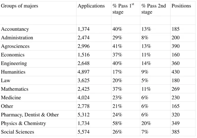
Speci…cally, Table 2 reports the number of student applications, the available positions and the rate of success at stages 1 and 2 in each of those major …elds. These …elds are quite di¤erent not only in terms of organization and in terms of contents but also regarding the ratio of the number of applicants to the number of positions. At one extreme lie Physics and Chemistry in which the number of applications is low and the …nal pass rates very high (20%). At a lesser degree this is also true for Accountancy, Agrosciences and Engineering. At the other extreme, lie Law, Medicine, Other humanities and Pharmacy, Dentist and Other in which the …nal pass rate is as low as 5 or 6% that is one out of 16 students passes the exam. Nevertheless, there are other di¤erentiations in terms of quality.
We now look in more detail to teh di¤erences in terms of grades across major …elds and we justify the restiction of our analysis to a speci…c subsample containg three medical majors.
4.1.1 The distribution of grades
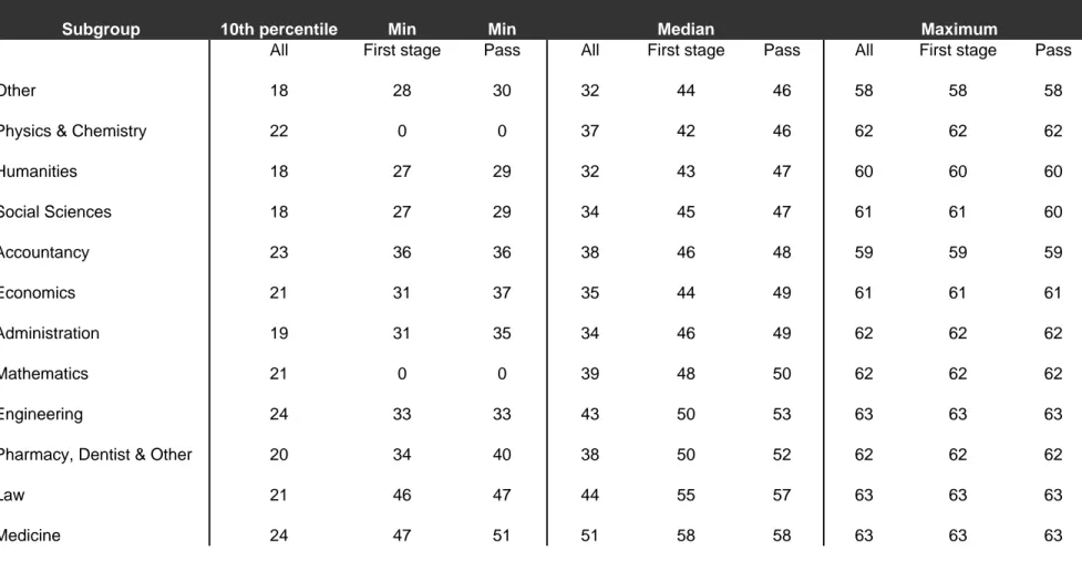
Tables 3 and 4 report summary statistics in each major …eld concerning the grades obtained …rst at the national examination (Table 3) and at the …rst stage of the college exam.7 We report statistics on the distribution of the initial and …rst stage grades in three samples:8 the complete sample, the sample of students who passed the …rst stage and the sample of students who passed the second stage and thus are accepted in the programs. Major …elds are ranked according to the median grade among those who passed the …nal exam in that major …eld.
7We do not report the second stage grades as they consist in grades in speci…c …elds that are not necessarily comparable across major …elds.
From Table 3, we can conclude that applications do not di¤er across majors in the tails of the distribution of initial grade since all minima are around 20 and all maxima are close to the top grade 63. The fact that applicants do self-select by talent when choosing their majors is captured by the medians of initial grades of applicants in column 4 of Table 3. Medians are quite constant around 34 in the 6 …rst major …elds yet then increase to attain the grade level of 44 for Law and 51 for Medicine. A second conclusion from Table 3 is that as expected the initial grades of those students who have access either to the second stage or pass the exam, are larger and are ordered as would be the …rst stage grades. Medians in the selected samples are now ranging from 42 in agrosciences to 58 in medicine. What strikes in this table is the proximity of the initial grades of those who pass and those who fails at the second stage which expresses that initial grade is an imperfect proxy for the …rst-stage grade. The range of medians shrinks to 46 to 58.
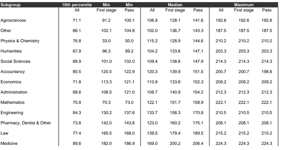
Initial grades are a predictor of talent and of e¤ort in the model. This is why the same statistics using …rst stage grades reported in Table 4 should be more informative. Indeed, even the minima tend to be ordered as the median of students who pass (column 6) from 70 to 90 in column 1. The …rst columns also reveal that some groupings might be somewhat arti…cial. The whole distribution is for example scattered out in mathematics from a minimum of 70 to a maximum of 222 while in medicine the range is 189 to 224. Other details are worth mentioning. The minimum grade in medicine to pass to the second stage is close to the maximum that was obtained by a successful students in Other …elds and somewhat less than in Agrosciences.
In conclusion, Medicine and Law are ranked the highest, as a matter of fact by a large amount of di¤erence with other major …elds. For instance, in Table 4, the …rst stage grade among those who passed in Medicine (resp. Law) has a median of 206 (resp. 189) while the next two are Pharmacy, Dentist and Other (175) and Engineering (171) and the minimum is for Agrosciences at 142.
4.1.2 Restricting the sample
com-petitive major …eld as shown above. There are three majors in this group corresponding to three di¤erent locations in the state of Ceará: Barbalha, Sobral and Fortaleza. The …rst two majors are small and o¤er 40 positions only while the last one, Fortaleza, is much larger since it o¤ers 160 seats. As shown in the empirical analysis below, this assymetry turns out to be important tp prove the importance of strategic e¤ects.
Table 5 repeats the analysis performed in Table 4 at the disaggregated level of those majors. Fortaleza is the most competitive one since the median of the …rst-stage grade of those who passed is equal to 208.57 while for the two others, it remains around 200. nevertheless, the pass rate as shown in Table 5 relating the number of applicants and the number of positions is about the same in Sobral and Fortaleza (7%) while it is slightly lower in Barbalha (5%). At the same time, Barbalha receives applications from the weakest students as shown by the median grades in the sample of all applicants to this major.
The list of variables and descriptive statistics in the pools of applicants to the three di¤erent majors appear in Table 6. The number of applicants taking the …rst exam are in total 3606 and are decomposed into respectively 739 (Barbalha), 542 (Sobral) and 2325 (Fortaleza). The number of seats after the …rst-stage is four times the number of …nal seats and is thus respectively equal to 160 for the small majors and 600 for Fortaleza. Note also that only two applicants in the pool of Fortaleza applicants and none in the others fail to go to the second-stage. The utility of taking the second stage exam after the revelation of information after the second-stage is (almost always) positive whatever the probability of success is.9
for Fortaleza …rst-order stochastically dominates the distribution of …rst-stage grades applicants. Fortaleza seems to be selected by better applicants.
4.2
Estimation of the dynamic model
4.2.1 Grade equations
We …rst estimate parametric grade equations form1 andm2as developed in Section 3.2.1 by
pseudo-maximum likelihood in which we use the …rst and second order moments of the grades and where the pseudo-distribution is normal. Results, using robust standard errors, are reported in Table 7. Table 7a reports the results using a simple speci…cation including the grade at national exam as the only covariate while Table 7b reports results for a more complete speci…cation. These tables report three sets of results corresponding to the coe¢cients in equation (8). The …rst two columns report the estimated coe¢cients of variables entering directly the speci…cation of …rst stage grades, 1 =x 1
and s1 (resp. second-stage grades, 2 =x 2 and s2). The last column reports the estimates for the
variables appearing in the common component, y =z y and . Finally, the estimated coe¢cients
of e¤ort, j, and standard errors, j, of each equation in (8) are reported at the bottom of the …rst
two columns.
In Table 7a talent as measured by the initial grade is in‡uencing positively the …rst and second stage grades. It is very signi…cant at the …rst stage but not at the second stage. As expected also, the e¤ect of e¤ort, as described by parameters j, are positive and highly signi…cant. Overall,
restriction (9) that says that unobserved e¤ort has the same e¤ect at both stages of the exam is frankly rejected (Student = 6.54). It might due to substantive di¤erences or it might be due to the too restrictive nature of the parametric model.
of success. On the other hand, the variables that are supposed to a¤ect grades but not utilities are the number of repetitions, the attendance of a preparatory course and a private high school. They are jointly signi…cant in the terms 1 and 2, as reported in the …rst two columns of table 7b.
In terms of the variables, results are quite expected. Regarding the direct e¤ects on grades, the older the applicant is, the lower grades at the two stages are. Attending a private high school increases …rst stage grades signi…cantly but not second stage grades while attending a preparatory course does the reverse by increasing second-stage grades signi…cantly. It conforms with the intuition that the …rst-stage content is general while the second-stage is speci…c. The number of repetitions increases at the 10% level the second-stage grade. Talent as described by the grade obtained at the national exam is unambiguously positive and signi…cant. Turning to the e¤ect of these variables on e¤ort (last column), we …nd again that age decreases e¤ort at least at age 25. The number of repetitions increases e¤ort signi…cantly and it might be that e¤ort expanded in the previous exams might …nd a way to express itself here. Parents’ education unambiguously increases e¤ort so that the utility of the majors unambiguously increases when these variables increase. Finally, talent also increases signi…cantly e¤ort.
4.2.2 Preference estimates
Second we estimated preferences using simulated maximum likelihood. Random preference het-erogeneities are assumed to be independent normals and we use the GHK simulator. The only explanatory variable in the simple speci…cation that is reported here is the Grade at the national exam and the results, using robust standard errors, are reported in Table 8. By assumption, the main parameter is normalized to 0and the standard error to 1 for the reference major (Fortaleza). As for the other two majors, the negative and signi…cant coe¢cients for the intercepts indicate that the choice of the small majors (Barbalha and Sobral) are dominated by Fortaleza and that talent attracts less students at Barbalha than at the other two schools something that we already spotted using descriptive statistics. The estimate of standard errors of tastes for the latter major are nevertheless larger and a signi…cant fraction of the population have preferences for Barbalha. This will have an impact on the results for some counterfactuals that we study now.
5
Evaluation of policy changes
As we estimated the model using candidates to the exam only, it is not immediately clear that we can evaluate the impact of policy changes on the extensive margin i.e. how it modi…es the composition of the population of candidates. If the assumptions of the economic model are correct it does not as a matter of fact. Indeed, changing the selection mechanism modi…es the success probabilities but it does not modify preferences and the key position of the outside option in the preference list. Indeed, if a major yields utility above the outside option, it will always deliver a value of this major above the outside option whatever the selection mechanism. The same argument applies to majors yielding utility below the outside option. Therefore, the population of interest remains the same .
Two possible changes among many others, are interesting to study:
Students could choose more than one major before the …rst stage.
Students could choose between the two stages and not before the …rst stage.
We develop these two cases in this section. For welfare, we use an utilitarist social welfare function where students get their ex-ante expected utility.
5.1
Enlarging choices
Suppose now that the choice set is composed by pairs (d ; d ) instead of a single choice d . The timing of the game remains the same, choices and investment being made before the …rst stage. After the …rst stage, there are now three possibilities:
m1 > tA1(d ; m0) : the student quali…es for the second stage of major d :
m1 < tA1(d ; m0) and m1 > tA1(d ; m0) : the student quali…es for the second stage of major
d .
m1 < tA1(d ; m0) :the student fails.
Note that the …rst and third stage are as in the original game whereas the second regime is original. It is also obvious the limit gradestA
Note also that because of perfect expectations, choosing a d such that tA
1(d ; m0) > tA1(d ; m0)
implies that the second regime disappears and is thus equivalent to make a single choice (d ;?)as
in the original experiment. It happens in all cases where only a single choice is valued positively by the agent. This is why we also allow for this choice possibility where tA
1(?; m0) =1.
The solving of the Nash equilibrium is slightly more di¢cult that in the original game. We follow the Gale Shapley student optimal stable mechanism to do that. Speci…cally, let us denote the common parameter controling limit grades as a vectort :
t1(d; m0) =t1(d; m0; t0); tA1(d; m0) =t1(d; m0; tA)
where t0 is the original set of limits in the exam as it works currently andtA is the counterfactual
set of grades which will describe the Nash equilibrium in the new game. This will apply sililarly to the second stage limit grades, t2(d; m0; tA).
Set up the individual model as follows. For those succesful at the …rst stage, we have before the second stage:
V2(h1) = Pr
2f
m2 > t2(d ; m0; tA)gud if m1 > t1(d ; m0; tA)
= Pr
2f
m2 > t2(d ; m0; tA)gud if m1 2[t1(d ; m0; tA); t1(d ; m0; tA))
= 0 if m1 < t1(d ; m0; tA)
where it should be understood that V2(h1) = 0 when the interval on the second line is empty.
The value function at the …rst period becomes:
V1(d ; d ; y; m0) = y+E 1V2(h1)
= y+E 1Pr
2f
m2 > t2(d ; m0; tA)g1fm1 > t1(d; m0; tA)gud
+E 1Pr
2f
m2 > t2(d ; m0; tA)g1fm1 2[t1(d ; m0; tA); t1(d ; m0; tA))gud
= y+Pd (y; m0; tA)ud +Pd(2)(y; m0; tA)ud : (12)
where Pd (y; m0; tA)is the overall probability of success for majord as de…ned above. The second
probability Pd(2)(y; m0; tA) is:
Pd(2)(y; m0; tA) =E 1Pr 2f
De…ne ~tA such that all limit grades remain the same except:
t1(d ; m0;~tA) = t1(d ; m0; tA):
Therefore:
Pd(2)(y; m0; tA) =Pd (y; m0; tA) Pd (y; m0;~tA); (13)
as a function of the previous success probabilities.
From equation (12), we can de…ney(d ;d ) and therefore the optimal value function as a function
of (ud ; ud ). We then de…ne:
(d ; d ) = arg max
(d1;d2;y)
V1(d1; d2; y; m0):
In order to compute the counterfactual limit gradestA we proceed as follows. We predict choice
and success at both stage probabilities for all individuals:
pi1(d; tA) = PrfChoosing (d;d~) and success at Stage 1 ford or
Choosing( ~d; d) and success at Stage 1 for d and not for d~g
Anlogously we can de…ne pi2(d; tA) describing choice and full success at both stages.
We then solve the non-linearD equations withD unknowns:
N
X
i=1
pij(d; tA) = Nj(d);
where Nj(d)are the number of o¤ered seats at Stage j for major d.
5.2
Changing the timing of choices
We can also change the timing of the game in the following way. The individual is supposed to choose his/her major after full revelation of the …rst stage grade. Note that it is not equivalent to the game where the list of preferences over all majors is as long as the individual wants since the choice can be made dependent upon the revelation of the …rst stage grade m1.
LetC(m1; m0; tB)be the choice set left after full revelation of the …rst stage grade:
where tB is any set of equilibrium limit grades in this new setting. The value before the second
stage is:
V2(h1) = Pr
2f
m2 > t2(d; m1; m0; tB)gud if d2C(m1; m0; tB)
= 0 if not. The individual chooses d such that:
d = arg max
d2C(m1;m0;tB)
V2(d; m1; m0)
The value function at the …rst period becomes:
V1(y; m0) = y+E 1V2(d ; m1; m0):
and we maximize this quantity in order to derive the optimal e¤ort, y.
There is no simple way of writing this maximization program since it corresponds to the inversion of the expectation and the maximization operators. Indeed, the dynamic program that was solved before correponds to:
max
d;y y+E 1V2(d; m1; m0)
to compare with the current one: max
y y+E 1maxd V2(d; m1; m0) :
The algorithm that could be used to solve this program is by simulation. Let s
1 a draw in the
distribution of 1: We can thus compute maxdV2(d; m1; m0) as a function of y and speci…cally, the
derivative of this function with respect to y. We repeat this computation over S simulations and get the evaluation of the second term E 1maxdV2(d; m1; m0) as a function ofy. We can then solve
for the optimal y. As y is bounded from below by 0 and the return to y is bounded if y tends to 1; a solution exists. It might not be given by a …rst order condition though depending on the characteristics of the function E 1maxdV2(d; m1; m0).
5.3
Discussion of the uniqueness of equilibrium
set-up and we do not have any general result on uniqueness, to our knowledge. Nevertheless, it is possible to prove uniqueness in a simple context. We assume that the scheme is the current selection scheme with heterogeneity across agents in preferences only (equal talent) and in which there is no e¤ort. We …rst look at the equilibrium at the second stage of the exam, given some probability of success, fpdgd=1;:;D, at the exam and given some choice probabilities f dgd=1;:;D. We pile up these
objects into vectorsp and .
The choice probabilities are given by the comparison between value functions fvd(pd)gd=1;:;D
where each value function vd depends on the success probability pd only and where it is strictly
increasing, i.e. pd > p0d =) vd(pd)> vd(p0d). We assume that for all d and all pd, we have d > 0.
An additional interesting property is that:
8p;
D
X
d=1
d(p) = independent ofp:
Without loss of generality, we will assume that = 1 in the following.
Let f dgd=1;:;D be the fraction of seats in the population attributable to each major. The
equilibrium relationships can then be written as:
d= Pr(Choosing d, Success in d) = Pr(Choosingd) Pr(Success in d) = pd d =zd(p);
since choices and realizations are independent because e¤ort and talent are absent. We pile up the elements zd(p) intoz(p). The probability of failing is:
D
X
d=1
(1 pd) d= 1 D
X
d=1
d;
and is satis…ed by construction as an accounting identity.
The following Lemma ensures the uniqueness of equilibrium:
Lemma 4 For any (p; p0); p6=p0 and no elements of p is equal to zero, we have z(p)6=z(p0).
Proof. By contradiction, assume thatz(p) =z(p0) so that for any d,p
d d=p0d 0d.
Consider …rst that (i) p0
d pd for all d and the inequality is strict for at least one d: We thus
have:
and for onedat least the inequality is strict since for alld, d >0. Thus d 0dand one inequality
at least is strict. It is a contradiction with PDd=1 d= 1. Case (i) can obviously be extended to the
case where p0
d pd and one inequality is strict.
Second, consider (ii): for alld2I; p0
d< pd and for alld 2J; p0d pd and where I is not empty.
The case where I is empty is the complement of case (i). We have:
d2I; pd d=p0d 0d=) d=
p0
d
pd
0
d < 0d;
since 0
d>0. It implies that:
X
d2I d<
X
d2I
0
d:
Yet, by de…nition: X
d2I
d= Pr(max
d2I vd(pd) maxd2J vd(pd));
X
d2I
0
d= Pr(max d2I vd(p
0
d) max
d2J vd(p
0
d)):
As for all d 2 I; p0
d < pd; maxd2Ivd(pd0) < maxd2Ivd(pd) since the value functions are increasing,
and as for all d2J; p0
d pd, maxd2Jvd(pd0) maxd2Jvd(pd); we have:
Pr(max
d2I vd(pd) maxd2J vd(pd)) Pr(maxd2I vd(p
0
d) max
d2J vd(p
0
d)) =)
X
d2I d
X
d2I
0
d;
a contradiction with the inequality above.
This Lemma ensures that the equilibrium is unique in terms of probabilitiesp. These equilibrium values are obtained as a fucntion of the thresholds:
pd = Pr(m1 > t1(d); m2 > t2(d)): (14)
Using the fact that …rst stage and second stage probabilities are …xed and known, we have: Pr(m1 > t1(d); m2 > t2(d))
Pr(m1 > t1(d))
=
which determines t1(d)as the unique solution of:
Pr(m1 > t1(d)) =
pd :
The second threshold t2(d) is then obtained by solving equation (14).
The general case is more di¢cult to tackle since it consist in solving equilibrium relationships such as:
5.4
Results
We computed the equilibrium thresholds in the …rst counterfactual developed in the subsection 5.1 above and using values reported in Tables 7a and 8. We computed these counterfactuals using the population of applicants at UFC by using that even success probabilities change, only students who have at least one positively valued major take exams at this University. The population of reference does not change as a result.
Table 9 reports the current and counterfactual thresholds. Quite surprisingly, the e¤ect is strong. The …rst school, Barbalha, becomes a very competitive place since the thresholds at the …rst and second stage are now the highest of all three majors. We attribute this to the very large dispersion of tastes for Barbalha in the population and to the fact that students have less incentives to censor themselves when they declare their …rst choices. They can "try" at Barbalha and as an insurance device select Fotaleza second, a thing that they would not do in the current system because of the small number of seats at that school (40). This is an illustration of the strategic e¤fect that the current system has on students. Furthermore, what Barbalha gets, the largest one Fortaleza loses it and at a lesser degree the other small one, Sobral. The counterfactual tends to create an elitist small medicine school at Barbalha while the elite big school was before in Fortaleza. This is not neutral for school managers and this could be evaluated.
If we adopt a pure utilitarist viewpoint by summing the ex-ante expected values for all students, the counterfactual is slightly preferred (Ev1 = 1406:750) to the current system (Ev0 = 1353:776).
Figure 4 report the estimated current and counterfactual distribution of expected values in the whole population and Figure 5 reports what we found in terms of di¤erences of expected values. The distribution of di¤erences is slightly assymetric. The ones who gain to the counterfactual change, gain more that the ones who lose. The distributive e¤ects are thus quite strong.
6
Conclusion
These results need to be extended in various directions. We should be able to extend the experiment using three majors only to the whole set of majors. It would also be interesting to perform semi-parametric estimation of grades to see if our results are robust to this change in speci…cation. Other counterfactuals like the one developed in the second subsection could also be analyzed.
REFERENCES
Abdulkadiro¼glu, A., Y., K., Che and Y. Yasuda, 2008, "Expanding Choice in School
Choice", Working paper.
Abdulkadiro¼glu, A., P.A. Pathak and A. Roth,2009, "Strategy-proofness versus E¢ciency
in Matching with Indi¤erences; Redesigning the NYC High School Match", American Economic Review, Vol. 99, No. 5, pp. 1954-1978.
Abdulkadiro¼glu, A. and T., Sonmez, 2003, "School Choice: A Mechanism Design
Ap-proach", American Economic Review, Vol. 93, No. 3, pp. 729-747
Arcidiacono, P.,2004, "Ability Sorting and the Returns to College Major,"Journal of
Econo-metrics, 121, 343-375.
Arcidiacono, P., 2005, "A¢rmative Action in Higher Education: How Do Admission and
Financial Aid Rules A¤ect Future Earnings?", Econometrica, Vol. 73, No. 5, pp. 1477-1524.
Balinski M., and T., Sönmez, 1999, "A Tale of Two Mechanisms: Student Placement",
Journal of Economic Theory 84, 73-94.
Bourdabat B. and Montmarquette C.,2007, “Choice of Fields of Study of Canadian
Univer-sity Graduates: The Role of Gender and their Parents’ Education”, IZA Discussion Paper No.2552.
Budish, E. and E. Cantillon, 2010, "The Multi-unit Assignment Problem: Theory and
Evidence from Course Allocation at Harvard", CEPR WP 7641
Carneiro, P., K. Hansen and J.J. Heckman,2003, "Estimating Distributions of
Counter-factuals with an Application to the Returns to Schooling and Measurement of the E¤ects of Un certainty on Schooling Choice,"International Economic Review, 44, 361-422.
Davies, T. and A. Stoian,2007, "Measuring the Sorting and Incentive E¤ects of Tournaments
Prizes", unpublished manuscript.
Epple, D., R. Romano and H. Sieg,2006, "Admission, Tuition, and Financial Aid Policies
in the Market for Higher Education",Econometrica, Vol. 74, No. 4, pp. 885-928
He, Y., 2009, "Gaming the School Choice Mechanism", unpublished manuscript, Columbia
University.
Heckman J.J., and S., Navarro, 2007, "Dynamic Discrete Choice and Dynamic Treatment
E¤ects", Journal of Econometrics, Volume 136, Issue 2, Pages 341-396.
Se-clection Errors on Academic Achievement: Evidence from the Beijing Open Enrollment Program", Economics of Education Review, 28:485-496.
Leuven, E. H. Osterbeek, J. Sonnemans and B. van der Klauuw, 2008, "Incentives
versus sorting in tournaments: Evidence from a …eld experiment", unpublished manuscript.
Instituto Nacional de Estudos e Pesquisas (INEP), 2008, "Sinopses estatísticas da
edu-cação superior", available at http://www.inep.gov.br/superior/censosuperior/sinopse/.
Olive, A. C.,2002, "Histórico da educação superior no Brasil", in: Soares, M. S. A. (coord.).
Educação superior no Brasil. Brasília, p. 31-42.
Magnac, T. and Thesmar, D. 2002, "Identifying Dynamic Discrete Decision Processes”,
Econometrica, 70, 801-816.
Manski C.,1993, “Adolescent Econometricians: How Do Youths Infer the Returns to
School-ing?”in Studies of Supply and Demand in Higher Education, edited by Charles T.Clotfelter and Michael Rothschild. Chicago: University of Chicago Press.
Manski, C., and D. Wise, 1983; College Choice in America. Cambridge, MA: Harvard
University Press.
Montmarquette C, K. Cannings and S. Mahseredjian, 2002, "How do young people
choose college majors?", Economics of Education Review 21 543–556.
Roth, A.E, 2008, "Deferred acceptance algorithms: history, theory, practice, and open
A
Statistical appendix
A.1
Proof of Lemma 3
Denote :M1 = m1 1 s1";
X = m"+v
so that the term on the last line is proportional to:
A E(X:1fX 0g j 1:X + 1: 1 =M1; ") =
Z Z
1:X+ 1: 1=M1
X:1fX 0g'(X m")'( 1)dXd 1
since X and are independent. We obtain:
A = Z Z
1:X+ 1: 1=M1;X 0
X:'(X m")'( )dXd =
Z
X 0
X:'(X m")'(
M1 1X
1
)dX:
We can write that:
'(X m")'(
M1 1X
1
) =A1:
1
'(X )
where A1; and are constant to determine. The left hand side is equal to:
1 2 exp( 1 2 2 1 2
1(X m")2+ (M1 1X)2 ) (15)
and the argument between square brackets in the exponential function is:
2
1X2+ 21m2" 2 21m"X+M12+ 21X2 2M1 1X
= X2( 21+ 21) 2X( 21m"+M1 1) + 21m2"+M12
= ( 2
1+ 21)(X )2+ 2X(( 21+ 21) ( 21m"+M1 1))
( 21+ 21) 2+ 21m2"+M12
= ( 21+ 21)(X )2 ( 21 + 21) 2+ 21m2"+M12;
if we set to:
=
2
1m"+M1 1 2
1+ 2 1
Let set 2 = 21 2
1+ 21; and replace in equation (15) to get :
2 1
exp( 1
2 2(X )
2):exp( 1
2 2 1
2
1m2"+M12 ( 21+ 21) 2
so that:
A= p
2 exp( 1 2 2
1 2
1m2"+M
2
1 ( 21+ 21) 2
Z
X 0
X:1'(X )dX =A1A2
where:
A1 = p
2 exp( 1 2 2
1 2
1m2"+M
2
1 ( 21+ 21) 2
Because:
A2 =
Z
X 0
X:1'(X )dX =E(X1fX 0g) = ( ) + '( )
we thus get:
E(m2 j"; m1) = 2+s2:"+ 2A1
h
( ) + '( )i:
In the truncated sample, we can also use that:
V (m2 j"; m1) = 22:V ((m"+v)1fm"+v 0g+ 2: 2 j"; m1)
= 22:V ((m"+v)1fm"+v 0g j"; m1) + 22;
= 22:V (X1fX 0g j"; m1) + 22;
= 22:(E X21fX 0g j"; m1 (E(X1fX 0g j"; m1))2) + 22;
where X =m"+v as before. It remains to evaluate:
B E X21fX 0g j"; m1
which by the same argument as above leads to:
B =A1
Z
X 0
X2:1'(X )dX:
Furthermore:
B1 =
Z
X 0
X2:1'(X )dX = 2:
Z
Y 0
Y2:'(Y )dY;
= 2((1 + 2
2) ( ) + '( )) = (
2+ 2) ( ) + '( ):
which proves the equations in the Lemma:
E(m2 j"; m1) = 2+s2:"+ 2:A1A2;