Dissolved Oxygen Downstream of an Effluent Outfall
in an Ice-Covered River: Natural and Artificial Aeration
Iran E. Lima Neto
1; David Z. Zhu, M.ASCE
2; Nallamuthu Rajaratnam, F.ASCE
3; Tong Yu
4; Mark Spafford
5;
and Preston McEachern
6Abstract: In ice-covered rivers, dissolved oxygen 共DO兲 might fall below critical levels for aquatic biota in the absence of surface
aeration, combined with low winter flow conditions and reduced photosynthesis rates. Open-water zones, however, can be created downstream of a diffuser by warm effluent discharges, resulting in an increase in surface aeration. In this study, we modeled the behavior of the effluent plume and the resulting open-water lead development in the Athabasca River, Alberta, Canada downstream of a pulp mill diffuser. The DO was found to increase by 0.26 mg/ L due to surface aeration of an open-water lead of 6.07 km. We also evaluated oxygen injection into the effluent pipeline to increase the DO in the river. At an injection rate of 3,500 and 5,000 lb/ day of liquid oxygen, the DO was increased by 0.16 and 0.21 mg/ L, which corresponded to an absorption efficiency of about 50%. The artificial aeration technique evaluated here appears to be an effective alternative to increase DO levels in ice-covered rivers. The results of this study are important in developing accurate DO models for ice-covered rivers and in evaluating oxygen injection systems.
DOI:10.1061/共ASCE兲0733-9372共2007兲133:11共1051兲
CE Database subject headings:Dissolved oxygen; Effluents; Diffusion; Ice; Rivers; Reaeration.
Introduction
The presence of sufficient dissolved oxygen 共DO兲 in rivers is important for aquatic life. Since the late 1980s, pulp mills along the Athabasca River, Alberta, Canada have been under various stages of development or expansion共see Fig. 1兲. High levels of biochemical oxygen demand共BOD兲loading from the mill efflu-ents, in addition to natural and municipal discharges, have been shown to cause a pronounced decline in DO concentrations pro-gressively downstream in the river共Chambers et al. 2000兲. The situation is more critical in winter seasons as a result of low flow conditions, which reduce the ability of the river to dilute BOD, and ice-cover conditions, which stop surface re-aeration and sub-stantially reduce photosynthesis rates.
There is a growing concern that increased development,
com-bined with reduced river flows in recent years, will cause DO concentrations to fall below critical levels for aquatic biota during winter months. The current guidelines for the maintenance of DO in Alberta Rivers are 5.0 mg/ L for acute exposure and 6.5 mg/ L for 7-day chronic exposure共Alberta Environment 1999兲. Histori-cal low flows occurred in the Athabasca River during the winters of 2002 and 2003. As a result, very low DO concentrations were observed that fell below chronic threshold values. In 2002, for instance, DO concentrations in the Athabasca River declined to an average of 5.7 mg/ L for a 28-day period upstream of Grand Rap-ids共see Fig. 1兲.
In order to minimize the impact of low DO levels in the Athabasca River, Alberta Environment has recently requested that the pulp mills along the river develop contingency plans for their operations. All of the mills are currently operating with ef-ficient wastewater treatment systems and can maintain good water quality in the Athabasca River under all but extreme climate and flow conditions. A low-cost alternative is required for the infrequent climatic conditions that can generate low DO condi-tions in the river. Oxygen injection into the effluent stream has been proposed as a possible remedy. Alberta-Pacific Forest Indus-tries Inc. 共Al-Pac兲 has recently conducted two oxygen injection tests during one winter season by injecting oxygen into the mill effluent before it is discharged through an existing diffuser outfall 共Stantec 2004兲 共see Fig. 2兲. While preliminary results seem to indicate that it is possible to increase the DO level by 0.5 mg/ L, several complications need to be carefully addressed before its effectiveness can be evaluated: The mixing of the effluent with the ambient river water and the development of the open-water lead downstream of the diffuser.
The temperature of the mill effluent is typically much warmer than the river water in winter months. It ranges from 10 to 22° C, even when the ambient air temperature is below −30° C. This warm effluent thus keeps an open-water lead downstream of the diffuser outfall throughout the winter共see Fig. 3兲. The length of 1
Ph.D. Candidate, Dept. of Civil and Environmental Engineering, Univ. of Alberta, Edmonton AB, Canada. E-mail: [email protected]
2
Professor, Dept. of Civil and Environmental Engineering, Univ. of Alberta, Edmonton AB, Canada. E-mail: [email protected]
3
Professor Emeritus, Dept. of Civil and Environmental Engineering, Univ. of Alberta, Edmonton AB, Canada. E-mail: nrajaratnam@ ualberta.ca
4
Associate Professor, Dept. of Civil and Environmental Engineering, Univ. of Alberta, Edmonton AB, Canada. E-mail: [email protected]
5
Aquatic Biologist, Alberta-Pacific Forest Industries Inc., Boyle AB, Canada. E-mail: [email protected]
6
Senior Limnologist, Alberta Environment, Edmonton AB, Canada. E-mail: [email protected]
Note. Discussion open until April 1, 2008. Separate discussions must be submitted for individual papers. To extend the closing date by one month, a written request must be filed with the ASCE Managing Editor. The manuscript for this paper was submitted for review and possible publication on September 12, 2005; approved on May 25, 2007. This paper is part of the Journal of Environmental Engineering, Vol. 133, No. 11, November 1, 2007. ©ASCE, ISSN 0733-9372/2007/11-1051– 1060/$25.00.
the open-water lead downstream of the Al-Pac diffuser ranges from a few hundred meters to several kilometers, and varies mainly as a function of air temperature and effluent rate and tem-perature. Given its significant length, it is important to properly estimate the size of the open-water lead as well as the amount of surface aeration it provides. In the Al-Pac’s oxygen injection study, it is also important to quantify the amount of the DO level increase due to oxygen injection and that due to surface aeration at the open-water lead. In a recent study by Tian 共2005兲 using USEPA’s Water Quality Analysis Simulation Program共WASP兲, it is shown that the DO level is very sensitive to the ice-cover ratio, i.e., the ratio of the ice-covered surface area to the total river surface area. So far, there is no predictive model for estimating the size of the open-water lead downstream of an effluent outfall. The objectives of this study are:共1兲To develop a methodology for predicting the size of the open-water lead downstream of a diffuser; 共2兲 to assess the ability of a modified Streeter-Phelps model to simulate the DO variation under partially and fully
ice-covered conditions; and 共3兲 to evaluate the effectiveness of the above-mentioned oxygen injection system. This study is impor-tant for the following reasons: 共1兲Effluent-induced open water zones have not been reported in the literature, and there are no reliable methods for quantifying their sizes. The amount of sur-face aeration through these open-water zones also needs to be quantified; and 共2兲injecting oxygen into an effluent diffuser has economical and operational advantages by making use of the ex-isting in-stream diffuser systems. However, there is no docu-mented literature on the application of this approach and its effectiveness.
Physical Characteristics and Field Work
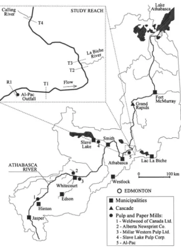
The Athabasca River originates in the Rocky Mountains of Jasper National Park, Alberta and flows northeast across the province to Lake Athabasca, as indicated in Fig. 1. It is unregulated, and therefore, discharge is highly seasonal, with the lowest flows oc-curring typically in February共about 70 m3/ s兲, when the river is
largely ice covered, and the highest flows occurring typically in June共about 1,000 m3/ s兲, when the river is under ice-free
condi-tion. As a result of a number of point and nonpoint discharges that contribute to the oxygen demand in the river, a DO sag occurs annually at the ice-covered section just above the Grand Rapids, a 10 m cascade located approximately 180 km downstream of the last significant point-source discharge, which is the Al-Pac efflu-ent diffuser. The main characteristics of the river during ice-covered periods are given in Table 1. A typical river cross section at 50 m downstream of Al-Pac diffuser is shown in Fig. 4. The ice
Table 1. Characteristics of the Athabasca River during Ice-Covered Periods 共Al-Pac Location兲 关Data Obtained from Beak Consultants Ltd.
共1995兲and Putz et al.共2000兲兴
Discharge 共m3s兲
Water depth
共m兲
Width
共m兲
Average velocity
共m/s兲 Slope
Ice thickness
共m兲
84 1.1 250 0.30 0.000166 0.50
Fig. 1.Location map of the Athabasca River, with indication of the study reach
Fig. 2.Diagram of the effluent discharge near the right bank of the Athabasca River, with indication of the oxygen injection point
Fig. 3. Open-water lead in the Athabasca River downstream of Al-Pac diffuser, with indication of flow direction
thickness, width of the open-water lead caused by the warmer effluent, and solute effluent concentration obtained from a field study conducted by Beak Consultants Ltd.共1995兲are also shown in this figure.
The Al-Pac diffuser is located about 2.7 m below the river bed and extends from approximately 30 to 82 m from the right bank 共looking downstream兲 of the Athabasca River 共see Fig. 2兲. Its structure consists of a coated steel pipe of 0.9 m diameter, con-taining 25 outlet ports with height of 3.0 m and inner diameter of 0.15 m. These outlet ports are oriented along the flow direction with a vertical angle of 45 deg and have a typical flow velocity of 2 m / s. Since the effluent comes out from the diffuser at a much higher velocity than the river water, it behaves as a series of turbulent jets that act as a propeller contracting the flow and in-ducing entrainment of the surrounding ambient water. As the ef-fluent is warmer than the river water, buoyancy will also force the jet trajectory to bend upwards. In this region, usually called the near-field zone, significant dilution is achieved within a short dis-tance from the discharge point. After a sufficiently large disdis-tance from the diffuser, the effluent is vertically fully mixed and the turbulence in the river becomes the dominant mixing mechanism. In this region, usually called the far-field zone, the effluent be-haves as a passive plume that grows in width due to turbulent diffusion processes.
Field work was conducted to evaluate the efficiency of the oxygen injection in the winter of 2004共Stantec 2004兲. The DO level was monitored at five transects across the river channel with one transect before the Al-Pac diffuser to provide background DO concentrations, and four transects below the diffuser from a dis-tance of 6 km up to 32 km共Fig. 1兲. The details of these transects are given below:
共1兲 Rl—Background control site, 0.5 km upstream of the dif-fuser outfall;
共2兲 Tl—6 km below the diffuser outfall;
共3兲 T2—15 km below the diffuser outfall 共0.5 km above La Biche River confluence兲;
共4兲 T3—15.5 km below the diffuser outfall 共0.2 km below La Biche River confluence兲; and
共5兲 T4—32 km below the diffuser outfall共0.1 km above Calling River confluence兲.
A baseline study with no oxygen injection was conducted on Feb. 7, 2004. At the beginning of the tests, the open water lead was about 2 km downstream of Al-Pac diffuser 共from Al-Pac, unpublished data兲. The average wind speed for the time of this survey was 2.8 m / s共Alberta Ambient Air Data Management Sys-tem 2004兲and air temperature was −8.9° C共Environment Canada
2004兲. In the subsequent days, two oxygen injection tests were conducted with oxygen being injected into the Al-Pac effluent pipeline at 500 m upstream of the pump house共see Fig. 2兲. The first oxygen injection test was conducted from Feb. 10–13, 2004, when the open-water lead was about 4 km downstream of Al-Pac diffuser. The average wind speed was 2.6 m / s and air temperature was −7.2° C. The second oxygen injection test was conducted from Feb. 17–20, 2004, when the open water lead was about 6 km downstream of Al-Pac diffuser. Due to the continuing in-crease in the open water length and the safety concerns with working in open areas, the transect T1 was moved to 7 km below the diffuser outfall during this oxygen injection test. The average wind speed was 1.9 m / s and air temperature was −5.1° C. The point of the oxygen injection was before the stabilization well in the pump house and the pressure at the effluent pipeline was estimated at about 3 atmosphere pressure. There is a potential that some oxygen might leak into the atmosphere through the stabili-zation well.
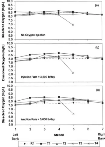
The DO concentrations for the baseline and oxygen injection tests were measured at midwater column of each station共spaced equally apart across the transects R1, T1, T2, T3, and T4兲with dissolved oxygen meters with an accuracy of ±0.01 mg/ L. Fig. 5 shows the cross-sectional DO variations for each test. Notice at transect T3, a significant DO deficit is observed at the station located near the right bank. This low DO is caused by the inflow plume from the La Biche River discharge, which does not have an opportunity to mix with the Athabasca river water. The La Biche
Fig. 4. Typical river cross section at 50 m downstream of Al-Pac diffuser共river discharge is 84 m3/ s兲, indicating solute 共Rhodamine
WT dye兲 effluent concentration, ice thickness, and width of the open-water lead关adapted from Beak Consultants Ltd.共1995兲兴
Fig. 5. Cross-sectional DO variation for each test 关adapted from Stantec 共2004兲兴: 共a兲 baseline study with no oxygen injection 共Feb. 7, 2004兲; 共b兲 oxygen injection at 3,500 lb/ day 共Feb. 10–13, 2004兲; and共c兲oxygen injection at 5,000 lb/ day共Feb. 17–20, 2004兲
River discharge is typically small 共1.15 m3/ s兲 compared to the
Athabasca River discharge, but it has a low DO concentration 共3.55 mg/ L兲 and a BOD of 1.02 mg/ L 共Chambers et al. 1996兲. Thus, transect T3 is ignored in the following discussion. At transect T4, the impact of La Biche River is accounted for by assuming complete mixing between the two rivers. Given the small discharge of the La Biche River 共about 2% of the winter flow of the Athabasca River兲, its impact on the DO levels of the Athabasca River at transect T4 is not significant. The increase in the average DO concentration共at transect T1兲above background levels共at transect R1兲was much more pronounced for the oxygen injection tests than for the baseline test. However, part of this DO increase was due to the surface aeration at the open-water lead downstream of the outfall共see Fig. 3兲.
Modeling Open-Water Lead Development
In this section, we model the development of the open-water lead downstream of Al-Pac diffuser on a daily basis by studying the mixing of the warm effluent in the river. The hydrodynamics of the turbulent buoyant jet/plume in the river is modeled using an expert system, CORMIX2共Akar and Jirka 1991兲. Once the tem-perature field of the effluent is obtained, the resulting open-water lead development is then predicted using a thermal breakup model共Hicks et al. 1997兲.
The CORMIX2 model is a subsystem of the software CORMIX-GI 4.3 共www.cormix.info兲 for simulating submerged multiport diffuser discharges into diverse ambient water condi-tions. It simplifies the receiving water body’s actual geometry by a rectangular cross section共schematization兲and uses the “equiva-lent slot diffuser” concept, which neglects the details of the in-dividual jets issuing from each diffuser port to the distance of their merging, but rather assumes that the flow comes from a long slot discharge with equivalent dynamic characteristics. This model is based upon integral length scale, and passive diffusion approaches to simulate the hydrodynamics of both the near-field zone共where momentum flux, buoyancy flux, and diffuser geom-etry control the jet trajectory and mixing processes兲, and the far-field zone共where buoyant spreading motions and passive dif-fusion control the trajectory and dilution of the effluent discharge plume兲.
In this study, the development of the open-water lead during the period of field study共Feb. 7–20, 2004兲 is predicted and the results are compared with the field measurements. The following data were obtained from Stantec共2004兲for these dates: The river discharge of 63 m3/ s, effluent flow rate of 0.87 m3/ s, and effluent
temperature of 22° C. The river cross section was schematized into a rectangular cross section of a depth of 1.0 m and a width of 230 m according to the requirement of the CORMIX2 model. Manning’s roughness for that section of the river was obtained from Beak Consultants Ltd. 共1995兲 and Putz et al.共2000兲 with
n= 0.027, typical for mildly meandering channels. The depth at discharge of 1.2 m was also used as input data, whereas the mul-tiport diffuser is located on the deeper part of the channel.
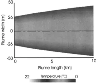
Using the above input data as well as information of the dif-fuser configuration, CORMIX2 classified the flow in the near field as a positively buoyant multiport diffuser discharge in uni-form ambient layer flow 共flow class: MU2兲and the flow in the far field as a passive-diffusion plume. The results for the near-field zone simulation showed that vertical mixing is completed at approximately 26 m downstream of Al-Pac diffuser due to the shallowness of the river, where the effluent plume width is 46 m and the centerline temperature is 1.0° C. The results for the far-field zone simulation showed that at 10 km below the outfall, the effluent plume width is 98 m and the centerline temperature is 0.59° C. Fig. 6 shows schematically the simulation of the effluent plume downstream of Al-Pac outfall共for Feb. 11, 2004兲, where the boundary of the plume is the half-width of the plume, which is defined as the distance from the centerline where the tem-perature is equal to 46% of the centerline value. The above CORMIX2 model was validated using the field results of Beak Consultants Ltd. 共1995兲. Adjusting the input data to the field conditions of the Athabasca River and Al-Pac effluent discharge during the tracer studies of Beak Consultants Ltd., CORMIX2 simulation provided plume widths of only 18% smaller and dilu-tion rates of only 24% larger 共see Table 2兲. Thus the results obtained in the present study with CORMIX2 are expected to be reliable.
According to Hicks et al. 共1997兲, thermal breakup processes
Table 2.Comparison between the Plume Width and Dilution Rate Obtained by Beak Consultants Ltd.共1995兲and CORMIX2 Simulation
Plume width共m兲a Dilution共%兲b
Distance
共km兲
Beak Consultants Ltd.
共1995兲
CORMIX2 simulation
Beak Consultants Ltd.
共1995兲
CORMIX2 simulation
0.05 40 48 30 27
8 110 90 52 42
16 140 113 71 53
a
Defined as the distance from the centerline where the concentration is equal to 46% of the centerline value. b
Defined as the initial concentration divided by the local centerline concentration.
Fig. 6.CORMIX2 simulation of transverse mixing downstream of Al-Pac diffuser for Feb. 11, 2004, in which half-width of the effluent plume corresponds to the distance from the centerline where the temperature is equal to 46% of the centerline value
usually occur when warm water flows under the ice cover result-ing in a downstream advance of a meltresult-ing front. The thermal breakup model, validated by Hicks et al.共1997兲for the Macken-zie River, Alberta, Canada, is used here to predict the open-water lead development in the Athabasca River. However, their model assumed that the temperature of the water was constant through-out the breakup period, as this warmer water came from a lake 共Great Slave Lake兲. Hence, we modified this model in order to account for spatial variation of effluent temperature downstream of Al-Pac outfall. Thus, temperature contour lines were generated using the results from CORMIX2 and equations to relate effluent temperature and the area formed by these contour lines and the diffuser were obtained.
The open-water lead development was simulated assuming that the melting front follows the temperature contour lines. The ice cover is assumed to melt according to two main processes: Ice-thickness reduction, assumed to occur due to direct heat input at the ice surface for a given ice density and latent heat of fusion; and open-water lead development, assumed to occur uniformly over the depth of the ice-cover leading edge due to heat carried by the warm water for a given water density and specific heat. The effluent temperature at the ice-cover leading edge is then obtained with the equations generated from CORMIX2 simulation. This iterative process is repeated for each subsequent day until the simulation reaches the desired area共or length兲of the open-water lead.
The following daily average values were used as input data for the thermal breakup model: Incoming solar radiation of 150 W / m2关obtained from Gray and Prowse 共1993兲 for the
Al-Pac’s latitude兴, water surface albedo of 0.1, ice surface albedo of 0.8, and heat transfer coefficient between the air and the water surface of 20 W / m2° C共obtained from Hicks et al. 1997兲.
The development of the open-water lead was simulated from the first day of the field test. On the first day共Feb. 7, 2004兲, the length of the open-water lead was estimated at 2.0 km based on visual observation. The ice thickness was measured by drilling holes across the river with a power ice auger. While this thickness varied from location to location, an average value of 0.5 m mea-sured upstream of the diffuser共transect R1 in Fig. 1兲was used as initial ice thickness. A similar value共see Fig. 4兲was also reported by Beak Consultants Ltd.共1995兲for similar cumulative air
tem-perature conditions. Ice surface temtem-perature was taken to be equal to the mean daily air temperature, which varied from −12.8 to −0.6° C共Environment Canada兲. Fig. 7 shows the estimated open-water lead development obtained by the CORMIX2/thermal breakup model simulation. The open-water lead increased signifi-cantly from the first to the last day of the simulation. The results are in agreement with the field observations from Al-Pac, in which the open area length was about 4.0 km for Feb. 11 and about 6.0 km for Feb. 18. Except for the near-field zone, where the effluent jet contracts laterally, as mentioned above, the width of the open-water lead decreases from about 40 to 0 m in the far-field zone共see Fig. 3兲, according to the temperature contour lines sketched in Fig. 7. The variation of this width along the river bends is caused by variations in the channel cross-sectional characteristics and increases in the transverse mixing coefficient due to the river’s secondary currents, which are caused by inter-actions between the main flow and the river bends, as reported in Dow et al.共2007兲.
A sensitivity analysis was conducted to investigate the impor-tance of some parameters that are not well known for the time and location of the survey for the following parameter ranges: Initial ice thickness共0.4– 0.6 m兲, initial open area length共1.5– 2.5 km兲, incoming solar radiation 共100– 200 W / m2兲, heat transfer
coeffi-cient between the air and the water surface 共15– 25 W / m2° C兲,
water surface albedo共0.05–0.15兲and ice surface albedo共0.7–0.9兲. Table 3 shows that the initial ice thickness and initial open area length have the largest influence on the results. However, since the maximum variation of the final open area length from the model calculation by using the standard values was about 10%, it can be inferred that the model is not highly sensitive to the range of parameters evaluated in this study.
Table 3. Sensitivity Analysis for the Parameters Used in the Thermal Breakup Model
Parameter
Standard
value Range
Variation of the final open-water length
共%兲
Initial ice thickness共m兲 0.5 0.4–0.6 +10.13– −9.39 Initial open area length共km兲 2.0 1.5–2.5 −4.05– + 3.96 Incoming solar radiation
共W / m2兲
150 100–200 −1.54– + 1.51
Air-water heat transfer coefficient共W / m2° C兲
20 15–25 +1.05– −1.08
Ice surface albedo 0.10 0.05–0.15 +0.29– −0.31
Water surface albedo 0.8 0.7–0.9 +0.22– −0.23
Fig. 7.Open-water lead development downstream of Al-Pac diffuser: Melting front follows temperature contour lines of 0.832, 0.811, 0.792, 0.775, 0.760, 0.746, 0.733, 0.722, 0.712, 0.703, 0.694, 0.686, 0.678, and 0.670° C
Fig. 8. Influence of air and effluent temperatures on the final open-water length
The final open-water length as a function of the air and efflu-ent temperatures is studied in Fig. 8, with the other input values the same as those in the above simulation. We can see that the lower the air and effluent temperatures, the shorter the final open-water length. For example, when the effluent temperature de-creases from 22 to 10° C while the average air temperature remains constant, the length of the final open lead decreases by about 2.4 km. On the other hand, when the average air tempera-ture decreases from 0 to −20° C while the effluent temperatempera-ture remains constant, the final open lead length decreases by only 0.7 km. This means that the effluent temperature is the main pa-rameter affecting the length of the open-water lead. Fig. 8 can be used as a quick predictive tool for estimating the final length of the open-water lead for similar conditions to our examined case. This graph also shows the sensitivity of the final open-water length to air and effluent temperatures, and it will be useful for plant operation.
Dissolved Oxygen Balance Model and Surface Aeration
Dobbins共1964兲extended Streeter-Phelps’s equation by obtaining a one-dimensional unsteady advection-dispersion equation incor-porating reaction terms to simulate the coupling variation of BOD concentration and DO deficit in the river, assuming complete mix-ing across the channel
L t +U
L x=
x
冉
KxL
x
冊
−K1L 共1兲D t +U
D x =
x
冉
KxD
x
冊
+K1L−K2D+K3−K4+S 共2兲whereL⫽BOD concentration; D⫽DO deficit共Cs−C兲, in which
C⫽DO concentration and CS⫽saturation value; U⫽mean river
velocity;Kx⫽longitudinal dispersion coefficient;K1⫽BOD decay
rate, K2⫽re-aeration coefficient, K3⫽oxygen uptake rate by
algae; K4⫽oxygen supply rate by algal photosynthesis; and
S⫽sediment oxygen demand 共SOD兲. Assuming a constant width
along the river, Eqs.共1兲and共2兲are simplified as the following for partially and fully ice-covered conditions.
For partially ice-covered conditions 共with open-water lead兲, the effective surface re-aeration coefficient becomes␣K2, where ␣⫽open-water ratio 共i.e., the ratio of the open-water width to
the average river width of 230 m兲, andK2⫽re-aeration coefficient
for an ice-free surface. The value of ␣ varies along the river
according to the width of the open-water lead 共see Fig. 7兲. As-suming steady-state conditions and neglecting the dispersion terms共Dobbins 1964兲and the difference between the oxygen up-take and supply rates by algae共Hou and Li 1987兲, we obtain the following analytical solutions for Eqs.共1兲and共2兲
L=L0exp
冉
−K1x
U
冊
共3兲D=D0exp
冉
−␣K2x U
冊
+K1L0
␣K2−K1
冋
exp冉
−K1x U
冊
− exp
冉
␣K2xU
冊
册
+ S␣K2
冋
1 − exp冉
− ␣K2xU
冊
册
共4兲in which L0 and D0⫽initial BOD concentration and DO
de-ficit, respectively. In Eq. 共4兲, the only source of oxygen is the re-aeration 共controlled by K2兲, and the sinks of oxygen are
the BOD decay共controlled byK1兲and the sediment oxygen
de-mand,S.
For fully ice-covered conditions, a field study conducted by MacDonald et al.共1989兲showed the under-ice re-aeration coeffi-cientK2approaching zero in the Athabasca River. This not only
implies that re-aeration is negligible, but also that groundwater, which is often poorly oxygenated and can contain significant chemical oxygen demand共COD兲, did not influenceK2in the
stud-ied reach共see Schreier et al. 1980兲. Thus, for ice-covered condi-tions, Eq.共4兲can be simplified by settingK2to zero
D=D0+L0
冋
1 − exp冉
−K1x U
冊
册
+S冉
x
U
冊
共5兲where the variation of BOD concentration in the river is also calculated by Eq.共3兲. In Eq.共5兲, there is no source of oxygen due to the ice cover, and two sinks of oxygen: BOD decay and the SOD.
In order to apply the model to predict the change of DO in the Athabasca River downstream of Al-Pac outfall for the baseline study 共Feb. 7, 2004兲, we used an average value of K1 of
0.01 day−1共Chambers et al. 1996兲, corrected to an average
efflu-ent plume temperature of 0.90° C共from CORMIX2 simulation兲, and an average value ofS of 0.18 mg/ L / day measured by Tian 共2005兲for the time and location of our study. However, the value forK2depends on several parameters, such as river flow
condi-tions and wind-shear velocity. For the condicondi-tions of the field study: The river discharge 共63 m3/ s兲, water depth共1.0 m兲, river
width共230 m兲, water surface slope共0.000166兲, Manning’s rough-ness 共n= 0.027兲, and average wind speed共2.81 m / s兲, as well as the average effluent plume temperature of 0.90° C, we calculated values forK2by using some of the most popular predictive
equa-tions for re-aeration induced by pure open-channel flows and combined wind/open-channel flows. Table 4 shows that these re-aeration coefficients varied from 0.64 to 1.95 day−1. In this study,
we adopt a value for K2= 1.63 day−1, which was obtained by
Chambers et al.共1996兲from their field study for an open-water reach of the Athabasca River downstream of a pulp mill共Millar
Table 4.Estimation of the Reaeration Coefficients by Using Predictive Equations
Reaeration equation
K2
共day−1at 20° C兲
K2
共day−1at 0.90° C兲
K2= 3.90U0.5H−1.5a 2.06 1.31
K2= 5.010U0.969H−1.673b 1.46 0.93
K2= 173共IU兲0.404H−0.66c 3.07 1.95
K2= 543I0.6236U0.5325H−0.7258d 1.22 0.77
K2= 1,740I0.79U0.46H0.74e 1.01 0.64
K2=K2,channel+K2,wind f
1.63 1.04
K2=K2,channel+K2,wind g
2.71 1.73
Note: H⫽average water depth 共m兲; I⫽water surface slope;
K2,channel⫽reaeration coefficient for pure open-channel flows 共day−1兲;
K2,wind⫽reaeration coefficient for pure wind-driven flows共day−1兲. a
O’Connor and Dobbins共1958兲. b
Churchill et al.共1962兲. c
Krenkel and Orlob共1962兲. d
Smoot共1988兲. e
Moog and Jirka共1998兲, valid forI⬎0.0000. f
Combination of wind and open-channel flow induced reaeration equations given by Chu and Jirka共2003兲.
g
Combination of wind and open-channel flow induced reaeration equations used in the USEPA’s WASP model.
Western Pulp Ltd.兲. This value is within the range ofK2shown in
Table 4 and seems to be adequate under relatively calm wind conditions. Note that when the wind speed is beyond 6 m / s,K2
value will increase significantly due to wind-generated waves and greater mixing at the air-water interface.
As the dissolved oxygen balance model is a 1D model, we need to obtain a cross-sectional averaged DO value in order to compare the field measurements with the model predictions. The measured DO varies across the channel due to the process of surface aeration and oxygen injection, with both of the processes giving a higher DO in the effluent plume. It is also interesting to point out that at the R1 section共see Fig. 1 insert兲, DO is more or less uniform共see Fig. 5兲. To obtain a cross-sectional averaged DO concentration, we cannot take a simple math average of the mea-sured DO shown in Fig. 5, as in the deeper part of the channel, the unit-width flow rate is bigger, thus, the DO flux is larger. As the flow velocity typically increases with depth, the unit-width dis-charge can be taken from Manning’s equation as proportional to the water depth to the power of 1.66. This power of 1.66 is also obtained by Chambers et al. 共1996兲 for the same reach of the Athabasca River evaluated in the present study. Therefore, the cross-sectional averaged DO value is estimated by the following equation:
Cavg=
兺
i=1
j
Ci共hi兲1.66
冒
兺
i=1j
共hi兲1.66 共6兲
where Ci and hi⫽local DO concentration and water depth for each stationi, respectively.
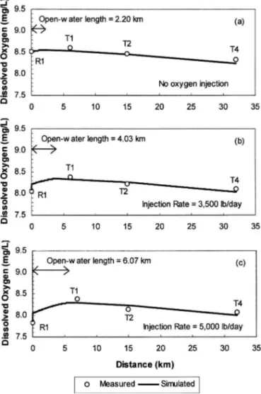
The following water quality parameters were used as input data for the DO balance model: Background BOD of 0.9 mg/ L 共Alberta Environment 2004兲, saturation DO concentration of 13.7 mg/ L 共Stantec 2004兲, effluent DO concentration of 5.6 mg/ L, and effluent BOD concentration of 3.8 mg/ L 共Tian 2005兲. Fig. 9共a兲shows the prediction of the DO balance model with the measured共cross-sectional averaged兲DO concentrations at transects R1, T1, T2, and T4. Here, an average length of the open-water lead 共2.2 km兲 and open-water ratio␣共varying from
0.112 to 0兲were obtained from the CORMIX2/thermal breakup model simulation. The DO model presents good fit to the field data with correlation coefficientR2= 0.930.
Two important processes are clearly shown in Fig. 9共a兲: The increase of DO共about 0.05 mg/ L兲in the open-water lead down-stream of the diffuser due to surface aeration, and the decrease of DO from the end of the open-water lead to T4 due to a lack of surface aeration and the effects of BOD and SOD. The slope of the DO depletion from T2 to T4 is well modeled, which indicates that the adoptedK1 andS values are reasonable. AsK1is small
compared to S, the DO decrease is dominated by SOD and its slope is almost linear under ice-covered conditions关see Eq.共5兲兴. This linear decrease in DO was also observed by Chambers et al. 共1997兲, who evaluated the impact of effluent discharges in several ice-covered rivers. In the open water region, surface aeration dominates over the SOD and BOD, thus the DO increases. Clearly the values of K1, K2, and S can be adjusted to have a
better fit of the measurement data in Fig. 9共a兲. However, by using the values obtained from the literature, we demonstrated the im-portance of the surface aeration in the open-water lead and the reliability of the DO balance model.
Efficiency of Oxygen Injection
Artificial aeration has long been successfully applied to minimize the problem of low DO levels in rivers by injecting air or oxygen into the water through submerged multiport diffusers 共Amberg et al. 1969; Whipple Jr. and Yu 1971; Marr et al. 1993兲. Here, we investigate the injection of oxygen into the existing effluent pipe-line to make use of the existing in-stream diffuser for maximizing the mixing and oxygen transfer. The approach provides signifi-cantly economic benefits and operational advantages. There are, however, several fundamental issues that need to be addressed: Related to the dynamics of this air-bubbles-and-effluent-water mixture and whether or not the air bubbles separate from the effluent plume in the river共see Socolofsky and Adams 2002兲. In the present study, we estimate the bulk efficiency of the oxygen injection through a field pilot study.
The field study takes advantage of the existing Al-Pac diffuser by injecting oxygen into the Al-Pac effluent pipeline during peri-ods of critical DO levels in the Athabasca River共see Fig. 2兲. Two tests were conducted with oxygen being injected at a rate of 3,500 lb/ day共Feb. 10–13, 2004兲and 5,000 lb/ day共Feb. 17–20, 2004兲.
Fig. 9.Comparison of the DO balance model to field data:共a兲total DO increase= 0.05 mg/ L 共␣ varies from 0.112 to 0兲; 共b兲 total DO
increase= 0.30 mg/ L, being 52% of this total due to oxygen injection and 48% due to surface aeration共␣ varies from 0.148 to 0兲; and共c兲
total DO increase= 0.46 mg/ L, being 44% of this total due to oxygen injection and 56% due to surface aeration共␣varies from 0.174 to 0兲
In this section, we apply the DO balance model to estimate the efficiency of this oxygen injection. We used the same values of K1,K2,S and water quality parameters assumed in the previous
section of this paper. Fig. 9共b兲shows the prediction of the DO balance model compared with the measured DO concentrations at transects R1, T1, T2, and T4 for the oxygen injection rate of 3,500 lb/ day, considering an average length of the open-water lead共4.03 km兲and open-water ratio␣共varying from 0.148 to 0兲
obtained from the CORMIX2/thermal breakup model simulation. The DO model presents a good fit to the field data, with the correlation coefficient R2= 0.935. Three processes are shown in Fig. 9共b兲: DO increase due to oxygen injection, assumed to occur instantaneously right after the diffuser; DO increase from the dif-fuser to the end of the open-water lead due to the dominant effect ofK2overK1andS; and DO decrease from the end of the
open-water lead to T4 due to the effects ofK1andSand lack of surface
aeration. The predicted total DO increase from R1 to the end of the open water lead is 0.30 mg/ L, which is composed of the surface aeration of the open-water lead and the oxygen injection. The DO increase over the open-water lead is 0.14 mg/ L 共i.e., 48% of the total DO increase兲. The remaining 52% of the total DO increase 共or 0.16 mg/ L兲 is due to oxygen injection. This gives the standard oxygen transfer efficiency 共SOTE兲 of 53%. SOTE is defined here as the fraction of oxygen supplied that is actually transferred or dissolved into the water.
Fig. 9共c兲presents the results for the oxygen injection rate of 5,000 lb/ day, considering an average length of the open-water lead共6.07 km兲and open-water ratio␣共varying from 0.174 to 0兲
obtained from the CORMIX2/thermal breakup model simulation. The DO model also presents a good fit to the field data with the correlation coefficient R2= 0.829. The three processes shown in Fig. 9共c兲are the same as those described for Fig. 9共b兲. The total DO increase from R1 to the end of the open-water lead is 0.46 mg/ L, with 0.26 mg/ L 共or 56% of the total DO increase兲 due to the open-water lead. The remaining 44% of the total DO increase共or 0.21 mg/ L兲is due to oxygen injection. This gives the SOTE of 49%. In both tests, the amounts of oxygen transferred to the river due to oxygen injection were of the same order of those due to open-water lead re-aeration.
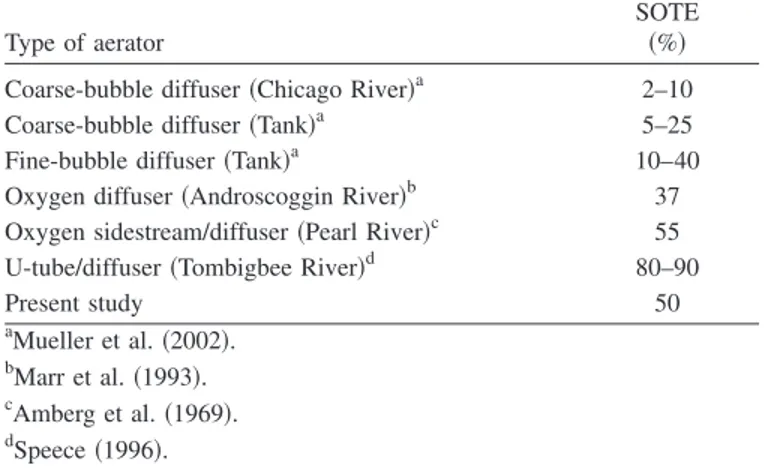
The SOTE decreased slightly from 53 to 49% when the amount of the oxygen injection increased from 3,500 lb/ day to 5,000 lb/ day. It should be noted that these numbers will change when the values of K1, K2, and S are adjusted. However, the
above results appear to be quite consistent and are expected to be reliable. From Table 5, one can see the SOTE obtained in the
present study is higher than those for conventional air injection systems and of the same order of those for oxygen injection sys-tems. This efficiency is, however, lower than that for the U-tube/ diffuser system, which has disadvantages such as higher construction/maintenance costs and inflexibility to be modified 共Mueller et al. 2002兲. In this study, some amount of the oxygen injected into the effluent pipeline could have escaped through the stabilization well in the pump house prior to the diffuser outfall. The amount of the oxygen injection in the present study is relatively small, with an increase of DO of about 0.2 mg/ L in the river. The oxygen injection system used in the Pearl River 共Amberg et al. 1969兲was similar to the one used in this study. However, that system increased the DO level by 2 mg/ L in the Pearl River by applying a much larger oxygen injection rate 共30,000 lb/ day兲. The discharge of the Pearl River 共43.2 m3/ s兲
and the sidestream to be oxygenated 共0.71 m3/ s兲 were of the
same order of the Athabasca River discharge共63.0 m3/ s兲and the
Al-Pac effluent flow rate共0.87 m3/ s兲, respectively. This
compari-son illustrates how much the artificial aeration technique evalu-ated here could potentially improve the DO levels in the Athabasca River if a higher oxygen injection rate were effectively applied.
When a higher oxygen injection rate is applied, Amberg et al. 共1969兲and Mueller et al.共2002兲reported that the SOTE becomes significantly lower as observed in other studies with different ar-tificial aeration systems. Lower SOTE at a higher injection rate may be due to coalescence of more numerous bubbles, reducing the surface-to-volume ratio and the contact time with the river water due to increased bubble-slip velocities. A laboratory study is currently being conducted to better understand the dynamics of the gas bubble-water mixture and mass transfer under various flow and operation conditions in order to improve the efficiency of oxygen injection systems.
Summary and Conclusions
In this paper, dissolved oxygen level in an ice-covered river downstream of an effluent diffuser is studied with or without oxy-gen injection. A methodology for predicting the open-water lead development was presented, and natural aeration through this open-water lead is studied. The efficiency of oxygen injection into an effluent diffuser is also evaluated through a field test. This study is important in modeling and managing DO levels in ice-covered rivers.
A CORMIX2 model was used to predict the behavior of an effluent plume downstream of the diffuser, while a thermal breakup model was adapted to simulate the resulting open-water lead development. This combined CORMIX2/thermal breakup model was able to predict field observations of an open-water advance from about 2 to 6 km in the river over the period of the field study. Model simulations revealed that effluent temperature was the dominant parameter affecting the length of the open-water lead, while air temperature was of lesser importance. This predictive tool for estimating the final size of the open-water lead is essential to predict DO depletion resulting from BOD loading to the river and the amount of oxygen that should be injected to offset depletion.
With the results from the CORMIX2/thermal breakup model and the water quality parameters and rates obtained from the lit-erature, it is shown that the spatial variation of DO along the river can be modeled with Streeter-Phelps equations proposed here for partially and fully ice-covered conditions. For the baseline study without oxygen injection, the model properly simulated two
im-Table 5. Absorption Efficiencies for Different Artificial Aeration Systems
Type of aerator
SOTE
共%兲
Coarse-bubble diffuser共Chicago River兲a 2–10
Coarse-bubble diffuser共Tank兲a 5–25
Fine-bubble diffuser共Tank兲a
10–40 Oxygen diffuser共Androscoggin River兲b 37 Oxygen sidestream/diffuser共Pearl River兲c 55
U-tube/diffuser共Tombigbee River兲d 80–90
Present study 50
a
Mueller et al.共2002兲. b
Marr et al.共1993兲. c
Amberg et al.共1969兲. d
Speece共1996兲.
portant processes: DO increase from the diffuser to the end of the open-water lead共2.2 km long兲due to the dominant effect of sur-face aeration over BOD and SOD; and DO decrease from the end of the open-water lead to the last transect due to a lack of surface aeration and the effects of BOD and SOD. The DO decrease was dominated by SOD with its slope close to linear.
The DO balance model was also applied to evaluate the effi-ciency of the artificial aeration system by injecting oxygen di-rectly into the effluent pipeline at 3,500 and 5,000 lb/ day. For the 3,500 lb/ day test, a total DO increase of 0.30 mg/L in the river was estimated, from which 52% was added by oxygen injection and the remaining 48% was added by surface aeration through an open-water lead of 4.03 km long. For the 5,000 lb/ day test, the
total DO increase was 0.46 mg/ L, from which 44% was added by oxygen injection and the remaining 56% was added due to sur-face aeration through an open-water lead of 6.07 km long. There-fore, the amounts of oxygen transferred to the river due to oxygen injection were of the same order of those due to open-water lead re-aeration.
The standard oxygen transfer efficiency was about 50% at both 3,500 lb/ day and 5,000 lb/ day. These efficiencies are higher than those for conventional air injection systems, and of the same order of those for oxygen injection systems described in the lit-erature. From these results, it can be inferred that the artificial aeration technique evaluated here can be a low-cost and efficient alternative to minimize the impact of low DO levels in
ice-Table 6.Summary of All Input Parameters Used in the CORMIX2/Thermal Breakup and DO Balance Model Simulations
Parameter Value
River discharge共m3/ s兲a
63
Water depth共m兲b 1.0
Average river width共m兲c 230
Manning’s roughnessd 0.027
Background BOD共mg/L兲e 0.9
Saturation DO concentration共mg/L兲a 13.7
BOD decay rate,K1共day−1兲 f
0.01 Reaeration coefficient,K2共day−1兲
f
1.63
Sediment oxygen demand,S共mg/L/day兲g 0.18
Effluent flow rate共m3/ s兲a
0.87 Effluent temperature共°C兲a
22
Depth at discharge共m兲h 1.2
Diffuser length共m兲h 52
Number of portsh 25
Port height共m兲h 3.0
Port diameter共m兲h 0.15
Port vertical angle共°兲h 45
Distance to the right bank共m兲h 30
Effluent DO concentration共mg/L兲a 5.6
Effluent BOD concentration共mg/L兲g 3.8
Daily average air temperatures共°C兲
共Feb. 7–20, 2004兲i
−8.9, −3.3, −2.2, −6.2, −1.8, −2.4, −7.4, −11.6, −9.1, −9.9, −8.4, −7.4, −3.9, −0.6
Daily average wind speeds共m/s兲 共Feb. 7–20, 2004兲j
2.8,3.1, 2.0, 4.2, 1.9, 2.2, 2.3, 2.8, 1.3, 1.9, 2.0, 1.4, 2.3, 2.0
Initial ice thickness共m兲k 0.5
Initial open area length共km兲k 2.0
Incoming solar radiation共W / m2兲l
150 Air-water heat transfer coefficient共W / m2° C兲m
20
Ice surface albedom 0.1
Water surface albedom 0.8
a
Stantec共2004兲. b
Water Survey of Canada共2004兲. c
Estimated using the water depth of 1.0 and the river transects measured by Beak Consultants Ltd.共1995兲. d
Beak Consultants Ltd.共1995兲and Putz et al.共2000兲. e
Alberta Environment共2004兲. f
Chambers et al.共1996兲. g
Tian共2005兲. h
Based on engineering plans of the diffuser outfall共Al-Pac兲. i
Environment Canada共2004兲. j
Alberta Ambient Air Data Management System共2004兲. k
Field measurements共Al-Pac兲. l
Obtained from Gray and Prowse共1993兲for the Al-Pac’s latitude. m
Obtained from Hicks et al.共1997兲for the Mackenzie River, Alberta, Canada.
covered rivers. The oxygen transfer efficiency at much higher injection rates is still not clear, as there are reports that this effi-ciency will decrease due to increased bubble-coalescence pro-cesses and increased bubble-slip velocities. Further lab and field studies are needed.
Acknowledgments
The first writer is supported by the Coordination for the Improve-ment of Higher Education Personnel Foundation 共CAPES兲, Ministry of Education, Brazil.
Appendix
Table 6 summarizes all the input parameters used in this paper to simulate the CORMIX2/thermal breakup and DO balance models.
Notation
The following symbols are used in this paper: D ⫽ dissolved oxygen deficit共mg/L兲;
D0 ⫽ initial dissolved oxygen deficit共mg/L兲;
K1 ⫽ oxygen uptake rate by biochemical oxygen demand
共day−1兲;
K2 ⫽ re-aeration coefficient共day−1兲;
K3 ⫽ oxygen uptake rate by algae共mg/L/day兲;
K4 ⫽ oxygen supply rate by algal photosynthesis
共mg/L/day兲;
Kx ⫽ longitudinal dispersion coefficient共m2/ s兲;
L ⫽ biochemical oxygen demand concentration共mg/L兲;
L0 ⫽ initial biochemical oxygen demand concentration
共mg/L兲;
S ⫽ sediment oxygen demand共mg/L/day兲;
SOTE ⫽ standard oxygen transfer efficiency, defined as the
fraction of oxygen supplied, which is actually transferred or dissolved into the water共%兲; t ⫽ time共s兲;
U ⫽ mean river velocity共m/s兲;
x ⫽ longitudinal distance共m兲; and
␣ ⫽ open-water width divided by the total river width
共open-water ratio兲.
References
Akar, P. J., and Jirka, G. H.共1991兲. “CORMIX2: An expert system for hydrodynamic mixing zone analysis of conventional and toxic sub-merged multiport diffuser discharges.”Technical Rep. No. EPA/600/ 3-91/073, U.S. Environmental Research Laboratory, Athens, Georgia. Alberta Ambient Air Data Management System. 共2004兲. “CASA data
warehouse—Data reports.”具http://www.casadata.org典.
Alberta Environment.共1999兲. “Surface water quality guidelines for use in Alberta.” Environmental Assurance Division, Science and Standards Branch, Edmonton, Alberta, 25.
Alberta Environment.共2004兲. “Alberta river basins—Water quality data.”
具http://www3.gov.ab.ca/env/water典.
Amberg, H. R., Wise, D. W., and Aspitarte, T. R. 共1969兲. “Aeration of streams with air and molecular oxygen.” Tappi J., 52共10兲, 1866–1871.
Beak Consultants Ltd.共1995兲. “Effluent plume delineation study for Al-berta Pacific Forest Industries Inc.”Rep. No. 7.10610.1, Brampton, Ontario.
Chambers, P. A., Brown, S., Culp, J. M., and Lowell, R. B. 共2000兲.
“Dissolved oxygen decline in ice-covered rivers of Northern Alberta and its effects on aquatic biota.” J. Aquatic Ecosystem Stress and Recovery, 8, 27–38.
Chambers, P. A., Pietroniro, A., Scrimgeour, G. J., and Ferguson, M.
共1996兲. “Assessment and validation of modelling under-ice dissolved oxygen using DOSTOC, Athabasca River, 1988 to 1994.”Project No. 2231-C1, Northern River Basin Study, Alberta, Canada.
Chambers, P. A., Scrimgeour, G. J., and Pietroniro, A.共1997兲. “Winter oxygen conditions in ice-covered rivers: The impact of pulp mill and municipal effluents.”Can. J. Fish. Aquat. Sci., 54, 2796–2806. Chu, C. R., and Jirka, G. H. 共2003兲. “Wind and stream flow induced
reaeration.”J. Environ. Eng., 129共12兲, 1129–1136.
Churchill, M. A., Elmore, H. L., and Buckingham, R. A.共1962兲. “The prediction of stream reaeration rates.” J. Sanit. Engrg. Div., 88共4兲, 1–46.
Dobbins, W. E. 共1964兲. “BOD and oxygen relationships in streams.”
J. Sanit. Engrg. Div., 90共3兲, 53–78.
Dow, K., Steffler, P. M., and Zhu, D. Z.共2007兲. “Intermediate field mix-ing of wastewater effluent in the North Saskatchewan River.”J. Hy-drol. Eng., submitted.
Environment Canada. 共2004兲. “National climate archive—Climate data online.”具http://www.climate.weatheroffice.ec.gc.ca典.
Gray, D. M., and Prowse, T. D.共1993兲. “Snow and floating ice.” Hand-book of hydrology, D. R. Maidment, ed., McGraw-Hill, New York, 7.1–7.58.
Hicks, F. E., Cui, W., and Andres, D.共1997兲. “Modelling thermal breakup on the Mackenzie River at the outlet of Great Slave Lake, N.W.T.”
Can. J. Civ. Eng., 24共4兲, 570–585.
Hou, R., and Li, H. 共1987兲. “Modeling of BOD-DO dynamics in an ice-covered river in Northern China.”Water Res., 21共3兲, 247–251. Krenkel, P. A., and Orlob, G. T. 共1962兲. “Turbulent diffusion and the
reaeration rate coefficient.”J. Sanit. Engrg. Div., 88共2兲, 53–116. MacDonald, G., Holley, E. R., and Goudey, S.共1989兲. “Athabasca River
winter reaeration investigation.” Final Rep., Environmental Assess-ment Division, Alberta EnvironAssess-ment.
Marr, D. H., Peterson, J. I., Critchfield, D. H., Danforth, R. H., and Wiley, Jr., F. A.共1993兲. “The Gulf Island Pond oxygenation project: A unique cooperative solution to an environmental problem.”Tappi J.,
76共7兲, 159–168.
Moog, D. B., and Jirka, G. H.共1998兲. “Analysis of reaeration equations using mean multiplicative error.”J. Environ. Eng., 124共2兲, 104–110. Mueller, J. A., Boyle, W. C., and Pöpel, H. J.共2002兲.Aeration: Principles
and practice, CRC Press, Boca Raton, Fla.
O’Connor, D. J., and Dobbins, W. E.共1958兲. “Mechanism of reaeration in natural streams.”Trans. Am. Soc. Civ. Eng., 123, 641–684. Putz, G., Odigboh, I., and Smith, D. W.共2000兲. “Two-dimensional
mod-elling of effluent mixing in the Athabasca River downstream of Al-berta Pacific Forest Industries, Inc.”Proj. Rep. No. 2000-2. Univ. of Alberta.
Schreier, H., Erlebach, W., and Albright, L.共1980兲. “Variations in water quality during winter in two Yukon rivers with emphasis on dissolved oxygen concentration.”Water Res., 14, 1345–1351.
Smoot, J. L.共1988兲. “An examination of stream reaeration coefficients and hydraulic conditions in a pool and riffle stream.” Ph.D. thesis, Virginia Polytechnic Institute and State Univ., Blacksburg, Va. Socolofsky, S. A., and Adams, E. E.共2002兲. “Multiphase plumes in
uni-form and stratified cross flow.”J. Hydraul. Res., 40共6兲, 661–672. Speece, R. E. 共1996兲. “Oxygen supplementation by U-tube to the
Tombigbee River.”Water Sci. Technol., 34共12兲, 83–90.
Stantec.共2004兲. “Alberta-Pacific Forest Industries Inc. dissolved oxygen trials—February 2004.” Prepared for Alberta-Pacific Forest Industries Inc. by Stantec Consulting Ltd., Calgary, Alberta.
Tian, Y.共2005兲. “Dissolved oxygen modeling and sediment oxygen de-mand study in the Athabasca River.” MS thesis, Dept. of Civil and Environmental Engineering, Univ. of Alberta.
Water Survey of Canada.共2004兲. “Water level and streamflow statistics.”
具http://www.wsc.ec.gc.ca/staflo典.
Whipple, W. Jr., and Yu, S. L.共1971兲. “Aeration systems for large navi-gable rivers.”J. Sanit. Engrg. Div., 97共6兲, 883–902.