Three variables are better than one: detection of European winter windstorms causing important damages

(1)

NHESSD

1, 4257–4285, 2013

Detection of damaging European

winter windstorms

M.-S. Deroche et al.

Title Page

Abstract Introduction

Conclusions References

Tables Figures

◭ ◮

Back Close

Full Screen / Esc

Printer-friendly Version Interactive Discussion

Discussion

P

a

per

|

Dis

cussion

P

a

per

|

Discussion

P

a

per

|

Discussio

n

P

a

per

|

Nat. Hazards Earth Syst. Sci. Discuss., 1, 4257–4285, 2013 www.nat-hazards-earth-syst-sci-discuss.net/1/4257/2013/ doi:10.5194/nhessd-1-4257-2013

Geoscientiic Geoscientiic

Natural Hazards and Earth System Sciences

Open Access

Discussions

This discussion paper is/has been under review for the journal Natural Hazards and Earth System Sciences (NHESS). Please refer to the corresponding final paper in NHESS if available.

Three variables are better than one:

detection of European winter windstorms

causing important damages

M.-S. Deroche1,2,3, M. Choux3, F. Codron2, and P. Yiou1

1

Laboratoire des Sciences du Climat et de l’Environnement, CEA-CNRS-UVSQ, UMR8212, CE Saclay l’Orme des Merisiers, 91191 Gif-sur-Yvette, France

2

Laboratoire de Meteorologie Dynamique, CNRS-UPMC-ENS-X, UMR8539, Place Jussieu, Paris, France

3

AXA Group Risk Management Department, Paris, France

Received: 20 June 2013 – Accepted: 11 August 2013 – Published: 23 August 2013

Correspondence to: M.-S. Deroche (madeleine-sophie.deroche@lmd.jussieu.fr)

(2)

NHESSD

1, 4257–4285, 2013

Title Page

Tables Figures

◭ ◮

Back Close

Full Screen / Esc

Discussion

P

a

per

|

Dis

cussion

P

a

per

|

Discussion

P

a

per

|

Discussio

n

P

a

per

|

Abstract

In this paper, we present a flexible methodology aimed at detecting European winter windstorms with high damage potential, using only meteorological variables. We start by analysing ten events known by the insurance industry to have caused extreme dam-ages. Looking at their surface signature in three fields: the relative vorticity at 850 hPa,

5

the sea-level pressure anomaly, and the ratio of the 10 m wind speed to its 98th per-centile, we find that those ten major events share an intense signature in all three fields. They were therefore extreme extra-tropical cyclones that became major eco-nomic events by crossing high-populated areas. These ten major events are however not the most intense ones of any of the three variables considered; so while using only

10

one variable cannot select the targeted events very well, the combination of the three variables proves to be more e_fficient.

We further test this method based on the combination of variables on di_fferent reanal-ysis datasets, and find that it can consistently isolate a small set of events containing the ten major events as well as other events with damage potential. It thus seems ready

15

to be applied to climate model simulations, for example to extract potentially damaging events in future climate projections.

1 Introduction

Extra-Tropical Cyclones (ETCs) are an important component of the mid-latitude atmo-spheric circulation. The North Atlantic ETCs regularly reach Europe, where they are

20

responsible for strong wind and rainfall episodes. During the winter season, some of them, usually referred to as European windstorms, can be particularly intense and gen-erate important wind-related damages. Munich Reinsurance Company (Munich Re) recently released a ranking of the ten costliest European windstorms over the last thirty years (Table 1). Each of them generated more than 2 thousand million USD

25

(3)

NHESSD

1, 4257–4285, 2013

Title Page

Tables Figures

◭ ◮

Back Close

Full Screen / Esc

Discussion

P

a

per

|

Dis

cussion

P

a

per

|

Discussion

P

a

per

|

Discussio

n

P

a

per

|

these extreme events, leading them to buy significant reinsurance covers in order to mitigate their risks. Therefore, and especially in a context of climate change, there is a need to characterize ETCs leading to important damages and to measure the poten-tial evolution of their surface signature (in terms of intensity and frequency) in the next decades.

5

The study of ETCs in current and future climate has been along two main lines. The most common one is to compute statistics of ETCs such as areas of genesis and lysis, cyclones density and cyclones intensity. In this first kind of analysis, all ETCs are detected and tracked thanks to automated algorithms. Ulbrich et al. (2009) provide a review of the existing approaches of cyclone definition, leading to di_fferent detection

10

and tracking schemes; more inter-comparison and insights on their performance can be found in Neu et al. (2013). These automated algorithms are based on the two-dimensional field of the following variables: the mean sea-level pressure (MSLP), the relative vorticity at 850 hPa (RV850) or the Laplacian of the MSLP. The detection of features is done by looking for either simple maxima of RV850 or minima of MSLP,

15

or more complex features such as opened or closed isobars. Feature tracking is then performed by linking features at successive time steps thanks to probabilistic prediction of feature movement. All the choices and assumptions made to develop a scheme o_ffer an analysis of the ETC characteristics from di_fferent angles but also introduce uncertainties (Neu et al., 2013). Once ETCs are detected their intensity is measured

20

by the value of the detection variable over the ETC lifetime. Extreme ETCs are defined as a particular class of cyclones, i.e. the ones with the highest intensity, but are not necessarily associated with strong winds or losses.

The second type of approach aims at evaluating the losses associated with Euro-pean winter windstorms (Leckebusch et al., 2007; Pinto et al., 2007, 2012; Della-Marta

25

(4)

NHESSD

1, 4257–4285, 2013

Title Page

Tables Figures

◭ ◮

Back Close

Full Screen / Esc

Discussion

P

a

per

|

Dis

cussion

P

a

per

|

Discussion

P

a

per

|

Discussio

n

P

a

per

|

10 m wind speed and the population density; in addition Pinto et al. (2012) separate the two driving loss factors of event severity, measured by a “meteorological index”, from the economic exposure. Della-Marta et al. (2009) also derive several indices, based ei-ther on the mean or on percentiles of the wind speed field, and compute return periods of extreme wind events using extreme value theory. Schwierz et al. (2010) use the ratio

5

of the 10 m wind speed over its local 98th percentile to detect events with criteria on intensity and spatial extension. The catalogue of events obtained is then used as input for an insurance loss model.

The approach we present in this paper mixes both types of analysis: we aim to detect the events with the highest damage potential, but using only meteorological variables

10

and no loss model to remain flexible. Our methodology is designed from the character-istics of the ten major events known for having caused important losses (Table 1), and we not only use the 10 m wind speed (variable used in the second type of analysis), but also the 850-hPa relative vorticity and the mean sea-level pressure (variables used in the first type of analysis). Indeed, the ten major events were primarily extreme

extra-15

tropical cyclones, with an intense signature in the three variables, and became major economic events when crossing high-populated areas. Looking for similar intense me-teorological signatures should thus lead to the detection of events with a potential for similarly high damage. Since the methodology is meant to be applied to the output of varied models, another key aspect is the adaptability of the detection and tracking

20

criteria.

The paper is structured as follows: in Sect. 2, an overview of the data and the vari-ables is given. In Sect. 3, we present the methodology and the choice of detection parameters. Finally, in Sect. 4, we compare the results in di_fferent reanalysis datasets. Conclusions are drawn in Sect. 5. All acronyms used in the text are listed in Table A1

25

(5)

NHESSD

1, 4257–4285, 2013

Title Page

Tables Figures

◭ ◮

Back Close

Full Screen / Esc

Discussion

P

a

per

|

Dis

cussion

P

a

per

|

Discussion

P

a

per

|

Discussio

n

P

a

per

|

2 Data and variables

2.1 Data

Three datasets are used in this paper. The detection methodology (Sect. 3) is de-veloped with the ERA Interim (ERAI) reanalysis dataset (Dee et al., 2011). ERAI is a 6 hourly dataset at a 0.75◦

×0.75◦ spatial resolution covering the period from 1979

5

to 2011, provided by the European Centre for Medium-Range Weather Forecasts. In Sect. 4, two other datasets are used along with ERAI to complete the analysis and validate the methodology. First, we use the NCEP-DOE (NCEP2) reanalysis from NCEP/NCAR, a 6 hourly data from 1979 to 2011 with a 2.5×2.5◦ spatial resolution (Kanamitsu et al., 2002). Second, we compute a spatial average of ERA Interim on the

10

NCEP2 2.5◦ _{resolution (ERAI-2.5).}

The geographical window used for the detection of events is restricted to Western Europe. The Mediterranean region is excluded because of the high regional cyclonic activity occurring there (Lionello et al., 2002; Campins et al., 2010; Nissen et al., 2010) independently, which is out of the scope of our study.

15

We finally use the ten most damaging events since 1987 ranked by Munich Re (Ta-ble 1). These events, called reference storms hereafter, are used as case studies in order to develop the methodology (Sect. 3). They cover a time period from 1987 to 2010, and are concentrated in the winter season from October to March. As a result, we choose to work with the 6 month winters (October–March) from 1987 to 2010 and

20

not the whole period covered by ERA Interim or NCEP2.

2.2 Variables

We consider three (near-) surface variables: the relative vorticity at 850 hPa, the mean sea-level pressure and the 10 m wind speed. These variables are commonly used ei-ther to detect and track ETCs (Ulbrich et al., 2009; Neu et al., 2013) or to assess

poten-25

(6)

NHESSD

1, 4257–4285, 2013

Title Page

Tables Figures

◭ ◮

Back Close

Full Screen / Esc

Discussion

P

a

per

|

Dis

cussion

P

a

per

|

Discussion

P

a

per

|

Discussio

n

P

a

per

|

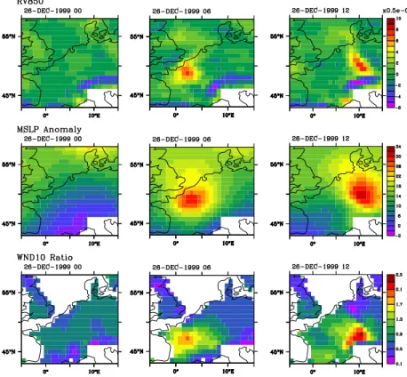
in Fig. 1 the spatial patterns of these three variables in the case of the major storm Lothar (December 1999).

The relative vorticity at 850 hPa (RV850) is either directly provided or computed as the curl of the velocity field at 850 hPa. The vorticity field is very sensitive to the spatial resolution; it becomes noisy at finer resolutions, leading to the detection of

numer-5

ous and intense local-scale features (Hoskins and Hodges, 2002; Ulbrich et al., 2009). Studies looking at cyclones over extended areas therefore apply a spatial smoothing of RV850, which also accounts for the poleward decrease of the grid size (Murray and Simmonds, 1991; Hodges, 1996; Sinclair et al., 1997; Hoskins and Hodges, 2002). In our study, since we consider a small geographical window over Europe, the grid size is

10

roughly uniform and we do not use any spatial smoothing. Features detected with the relative vorticity are also not necessarily associated with an ETC in the classical mean-ing of a pressure minimum. Hence, most of the detection schemes look for a minimum of mean sea-level pressure in the vicinity of the maximum of relative vorticity to define the centre of an ETC (e.g. Murray and Simmonds, 1991; Blender et al., 1997; Gulev

15

et al., 2001; Pinto et al., 2005). We instead start by detecting intense events indepen-dently with the relative vorticity at 850 hPa, the mean sea-level pressure and the 10 m wind speed.

We next use the anomaly of the mean sea-level pressure defined, at each time step, as the difference between the MSLP and its running average over eight days

20

(MSLP8 days):

MSLP_anom(i,j,t)₌−

MSLP(i,j,t)−MSLP8 days(i,j,t)

(1)

MSLP8 days(i,j,t)₌ 1

32·

t+16 X

t−16

MSLP(i,j,t) (2)

where (i,j) are the grid points coordinates andtthe 4-time daily time steps.

(7)

NHESSD

1, 4257–4285, 2013

Title Page

Tables Figures

◭ ◮

Back Close

Full Screen / Esc

Discussion

P

a

per

|

Dis

cussion

P

a

per

|

Discussion

P

a

per

|

Discussio

n

P

a

per

|

The mean sea-level pressure is a large-scale field, so it is better resolved than the vorticity. It is also strongly constrained in reanalysis datasets thanks to the great num-ber and quality of observation data, especially over continents. When developing a de-tection scheme with this variable, it is important to account for two characteristics of the MSLP field. First, over high orography, MSLP values are extrapolated and may not

5

be meaningful. Most of the approaches based on the MSLP field therefore ignore lows detected in areas higher than a predefined threshold, usually 1000 m or 1500 m (Mur-ray and Simmonds, 1991; Pinto et al., 2005; Hanley and Caballero, 2012). Second, the ETCs evolve on a more slowly varying background flow that also has large MSLP gra-dients. A spatial or temporal filter is often used to bring out the small-scale features and

10

remove the biases due to variations of the background MSLP (Hoskins and Hodges, 2002). A simple temporal filter is used in our study. We first tried removing the climatol-ogy of MSLP but it was not enough to bring out some of the targeted events. We thus chose to work with the running average of MSLP over eight days, which represents the signature of the weather regime surrounding the occurrence of ETCs (Feldstein, 2000)

15

and has also been used by Rivi `ere and Joly (2006). MSLP8daysis computed at a given time stept as the average of the MSLP over sixteen time steps preceding time stept and sixteen time steps following it (i.e. over 32 time steps or 8 days), see Eq. (2).

The third variable we use is the ratio of the 10 m wind speed to its 98th percentile (WND10₉₈), computed for continental grid points only:

20

WND10_ratio(i,j,t)₌WND10(i,j,t)

WND10₉₈(i,j) (3)

The 10 m wind speed is strongly dependent on the modelling of boundary layer pro-cesses, even in the reanalyses, as well as on the time and space resolution of the outputs. Using the ratio over the 98th percentile alleviates some of these biases. This specific ratio is also often used in ETC impact studies, not to detect features but rather

25

(8)

NHESSD

1, 4257–4285, 2013

Title Page

Tables Figures

◭ ◮

Back Close

Full Screen / Esc

Discussion

P

a

per

|

Dis

cussion

P

a

per

|

Discussion

P

a

per

|

Discussio

n

P

a

per

|

wind speed ratio, indices of ETC impacts usually integrate the population density, du-ration and spatial extension of the event (Klawa and Ulbrich, 2003; Leckebusch et al., 2007; Pinto et al., 2007; Donat et al., 2011). In this paper, the 10 m wind speed ra-tio is used as a detecra-tion variable, similar to the Schwierz et al. (2010) one or to the “Meteorological Index” from Pinto et al. (2012).

5

Each of the three variables described captures specific spatio-temporal scales and thus accounts for different aspects of extra-tropical cyclones. The relative vorticity at 850 hPa captures local and fast meso-scale structures whereas the MSLP anomaly captures larger and slower systems. The ratio of the 10 m wind speed measures, at a local scale, a wind intensity that is strongly correlated with the damage potential.

10

3 Case study and methodology

This section presents a method for detecting and tracking events with a high damage potential in Europe. The method itself and the choice of parameters are based on the case study of the ten reference storms (Sect. 3.1), using the ERA Interim dataset. The case study aims at answering the following questions: do major events with important

15

economic losses share some meteorological characteristics? How extreme is their sig-nature? Is there a variable that isolates them better than another one? The answers to these questions lead us to the definition of the appropriate criteria for the detection of potentially damageable events within a given meteorological dataset (Sect. 3.2).

3.1 Case study

20

A preliminary examination of maps of the three variables at the time of occurrence of the ten reference storms reveals that all ten events display a strong signature in each of the three considered variables, which singles them out from their surrounding environment when they pass across the Western Europe geographical window (the example of Lothar is shown in Fig. 1). Usually, detection methods select all the local

(9)

NHESSD

1, 4257–4285, 2013

Title Page

Tables Figures

◭ ◮

Back Close

Full Screen / Esc

Discussion

P

a

per

|

Dis

cussion

P

a

per

|

Discussion

P

a

per

|

Discussio

n

P

a

per

|

maxima above a specified threshold because several cyclones can exist at a given time step within a wide region (Hoskins and Hodges, 2002). Here, since the considered area is small and since there are no other significant local maxima during the time each reference storm crossed this area (see Fig. 1), we choose to only retain the global maximum of each variable at each 6 h time step.

5

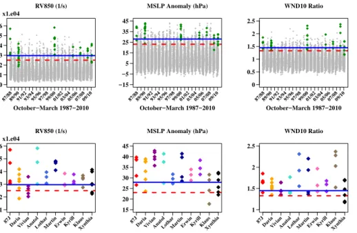
The intensity of the ten reference storms is compared to the distribution of the global maxima in Fig. 2. In the first row, time series of the maxima of the three variables are shown together with their respective 95th percentile (red dashed line) and 98th per-centile (blue line). The maximum values reached at the time of occurrence of the ten reference storms, coloured in green, are mainly located in the upper part of the plot.

10

This demonstrates that in ERAI the ten reference storms (major events in terms of economic losses) all have a particularly intense surface signature at the same time in each of the three variables. This signature is now used to define detection thresholds: the second row of Fig. 2 shows again the maximum values of each variable, but only during the occurrence of the ten reference storms. Most are above the 95th percentile

15

of their respective distributions. Furthermore, there is for each case and each variable at least one value above the 98th percentile. These two percentiles are therefore cho-sen for the methodology, as detection and selection thresholds respectively. Di_fferent combinations of detection and selection thresholds have been tested and sensitivity tests have been performed on the intensity of these thresholds. Raising the detection

20

threshold proves to be ine_fficient since some reference storms would not be detected afterwards. The combination of 95th and 98th percentiles is retained because it en-sures the detection of the ten reference storms while minimizing the total number of selected events.

3.2 Methodology

25

(10)

NHESSD

1, 4257–4285, 2013

Title Page

Tables Figures

◭ ◮

Back Close

Full Screen / Esc

Discussion

P

a

per

|

Dis

cussion

P

a

per

|

Discussion

P

a

per

|

Discussio

n

P

a

per

|

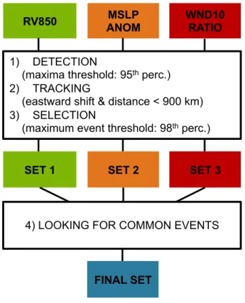
for each variable, and the 95th percentile of the time series’ distribution is used as a detection threshold. Second, a simple tracking is performed, that gathers into one “event” consecutive detected maxima above the 95th percentile if there is an eastward shift and if the distance between the two consecutive maxima is lower than 900 km. Third, we restrict our events set to events having at least one value above the 98th

5

percentile and lasting at least two time steps. Fourth, we compare the events selected by using the three di_fferent variables, and retain the ones that are present for all three (i.e. selected events that share at least at one time step above the 95th percentile for the three variables).

The rationale for the last step is that applying the selection process to ERAI produces

10

149 events with the relative vorticity, 117 events with the pressure anomaly and 91 events with the 10 m wind speed. The ten reference storms are included in each set of events, but the number of events obtained exceeds the initial objective. Additionally, the intensity ranking of events within the three sets (Table 2) indicates that the reference storms are not top-ranked for any of the three variables. This leads to the conclusion

15

that the reference storms cannot be isolated through the use of a single variable and high detection thresholds. However, even though the ten reference storms are not the top-ranked events of any variable, they are selected with each of them. This may not be the case for the other events of the catalogues.

The complementarity of the three variables is further analysed in the first panel of

20

Fig. 4 that shows the number of events common to sets built with di_fferent variables. Two events selected either using two di_fferent variables or in two di_fferent datasets are considered as common if they share at least one 6 h time step. In ERAI, the number of events common between pair-wise variables is less than half the number of events de-tected with each variable separately; and taking events common to the three variables

25

(11)

NHESSD

1, 4257–4285, 2013

Title Page

Tables Figures

◭ ◮

Back Close

Full Screen / Esc

Discussion

P

a

per

|

Dis

cussion

P

a

per

|

Discussion

P

a

per

|

Discussio

n

P

a

per

|

years belong to a particular group of meteorological systems that exhibit an intense surface signature in every field considered. Taking the intersection of event sets for three separate variables therefore gives more satisfying results than the use of a sin-gle one, in terms of global event intensity or potential for major impacts. Indeed, the number of 24 events finally selected over the last thirty years is consistent with records

5

from insurance companies of major damages over the area considered. Trying to iso-late the same number of events using one variable only would leave aside several of the 10 that actually led to major losses. The complementarity of the three variables is therefore a powerful tool to further restrict our events selection and to constitute the last step of the procedure.

10

The four-step methodology has been developed using the ERA Interim dataset. We have shown that it can isolate a group of events that can be defined as extremes in terms of meteorological signature and could lead to important damages if crossing ar-eas with high exposure. However, the method is meant for ar-easily analysing the outputs of various models over large periods of time so its robustness and flexibility need to be

15

further tested.

4 Testing the robustness of the methodology

One initial objective was to apply the method to the outputs of general circulation models such as the ones participating to the Coupled Model Intercomparison Project (CMIP5). Most of these models have a coarser spatial resolution than ERAI (around

20

2.5◦_{), especially when run over longer periods. In order to validate its robustness}

against spatial resolution, the methodology is thus applied to the coarser reanalysis datasets NCEP2 and ERAI downgraded to the 2.5◦_{spatial resolution. This will partially}

separate the resolution e_ffect (ERAI vs. ERAI-2.5) from the model e_ffect (ERAI-2.5 vs. NCEP2), with the caveat that downgrading the output of a 0.75◦_{run to 2.5}◦_{is di}

fferent

25

(12)

NHESSD

1, 4257–4285, 2013

Title Page

Tables Figures

◭ ◮

Back Close

Full Screen / Esc

Discussion

P

a

per

|

Dis

cussion

P

a

per

|

Discussion

P

a

per

|

Discussio

n

P

a

per

|

The results presented hereafter are obtained with the methodology presented in Sect. 3. We first present the distributions of the maxima of the three variables in order to analyse the di_fferences and similarities between the reanalysis datasets that impact the detection of events (Sect. 4.1). We then focus on the events selected with each vari-able and compare the results between the reanalysis datasets (Sect. 4.2). Finally, we

5

compare the final sets of events and conclude on the relevance of the multi-variables approach (Sect. 4.3).

4.1 Maxima distribution functions

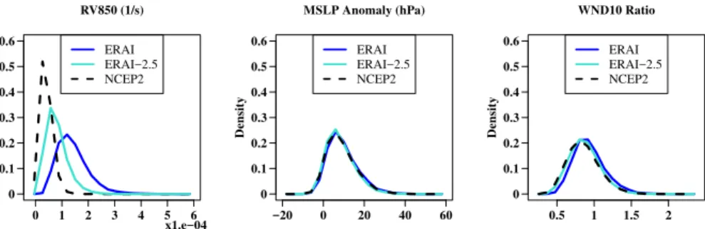
The Probability Distribution Functions (PDFs) obtained from the maxima time-series defined in Sect. 3.1 are plotted in Fig. 5 for ERAI, ERAI-2.5 and NCEP2. While the

10

distributions of MSLP anomaly and 10 m wind speed ratio are nearly identical from one dataset to the other, the relative vorticity distributions di_ffer: a first shift towards lower values is observed when downgrading the resolution (from ERAI to ERAI-2.5), a sec-ond one when changing the model (from ERAI-2.5 to NCEP2). RV850 indeed greatly depends on the spatial resolution (Ulbrich et al., 2009; Hodges et al., 2011); when

15

dealing with outputs at di_fferent spatial resolutions, it is thus important to keep in mind that its values (and particularly extreme values) might not be reproduced similarly from one dataset to the other. This stresses out the necessity of using intensity thresholds based on percentiles rather than absolute values, in order to ensure the adaptability of the detection to di_fferent kinds of datasets.

20

The second step of the procedure is the detection of the maxima above the 95th percentile of each PDF. Selected events are formed from these maxima; so a condition to have a common event in two datasets is that a maximum above the 95th percentile is detected at the same time step in both. Therefore, in order to measure the likelihood to get the same events from one dataset to the other, we compare the number of maxima

25

(13)

NHESSD

1, 4257–4285, 2013

Title Page

Tables Figures

◭ ◮

Back Close

Full Screen / Esc

Discussion

P

a

per

|

Dis

cussion

P

a

per

|

Discussion

P

a

per

|

Discussio

n

P

a

per

|

ERAI-2.5 and NCEP2 (83 % of common maxima above the 95th percentile). It is thus very likely that the events detected in ERAI, ERAI-2.5 and NCEP2 with the MSLP anomaly will be the same. Results on the two other variables depend on the reanalysis datasets. For ERAI and ERAI-2.5, the high number of common maxima above the 95th percentile with the relative vorticity (62 %) and the 10 m wind speed (71 %) suggests

5

that the events detected in both datasets will be the same. For ERAI-2.5 and NCEP2, the number of common maxima above the 95th percentile happening at the same time is smaller: around 42 % with both relative vorticity and 10 m wind speed ratio. It is therefore unlikely that the events detected with any of these two variables will be the same between ERAI-2.5 and NCEP2.

10

To conclude, the three reanalysis datasets display di_fferences in some variables that could impact the detection of events. Di_fferences in intensity (strongest with the relative vorticity at 850 hPa) do not impact the detection if they are a uniform change, as they would be o_ffset by the definition of thresholds as percentiles of the PDFs derived from each dataset. However, di_fferences in the ordering of the distribution, and in particular

15

of its tail, greatly impact the events detection: events are formed from the maxima above the 95th percentile, so if they do not occur at the same times in two datasets, di_fferent events will detected. The variable least sensitive to the choice of dataset is the anomaly of mean sea-level pressure that has a comparable intensity in the three datasets and a high percentage of common maxima. As mentioned in Sect. 2, the

20

mean sea-level pressure is a large-scale field (compared to the relative vorticity and the 10 m wind speed) with a large amount of assimilated observation data, which may explain the small di_fferences between the three reanalysis datasets.

4.2 Generating the three events sets

Once the maxima above the 95th percentile are detected, events are formed for each

25

(14)

NHESSD

1, 4257–4285, 2013

Title Page

Tables Figures

◭ ◮

Back Close

Full Screen / Esc

Discussion

P

a

per

|

Dis

cussion

P

a

per

|

Discussion

P

a

per

|

Discussio

n

P

a

per

|

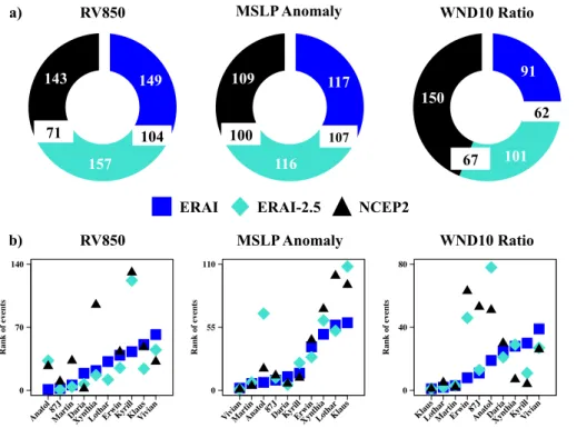
variable within the three datasets. This confirms one of the findings of the analysis with ERAI in Sect. 3: one variable is not enough to isolate satisfyingly the reference storms. As we did in Sect. 3 with ERAI only, we consider the ranking of the ten reference storms within the three variables and the three reanalysis datasets (Fig. 7b). We see that the ten reference storms are not the ten most extreme events in any pair of reanalysis

5

datasets and variables, which generalizes the result obtained with ERAI only. Addition-ally, the ranks of the ten reference storms vary with the dataset. For example, in order to select the ten reference storms with the anomaly of mean sea-level pressure, we must take the 55 first events with ERAI, the 110 first ones with ERAI-2.5 and the 100 first ones with NCEP2. The rank is therefore not a robust criterion to select e_ffectively

10

the reference storms and other similar events in outputs from various models.

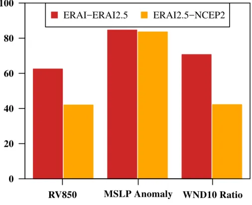
Moreover, the number of common events between pair-wise reanalysis datasets confirms the previous analysis on the number of common maxima above the 95th percentile (Fig. 7a). The mean sea-level pressure displays the highest percentage of common events between ERAI and ERAI-2.5 (93 %) as well as between ERAI-2.5

15

and NCEP2 (92 %). For the relative vorticity and the 10 m wind speed, many com-mon events are found between ERAI and ERAI-2.5 (around 60 % of comcom-mon events for both variables) but only a small percentage of common events is found between ERAI-2.5 and NCEP2 (around 35 % for both variables).

4.3 Generating the final events set

20

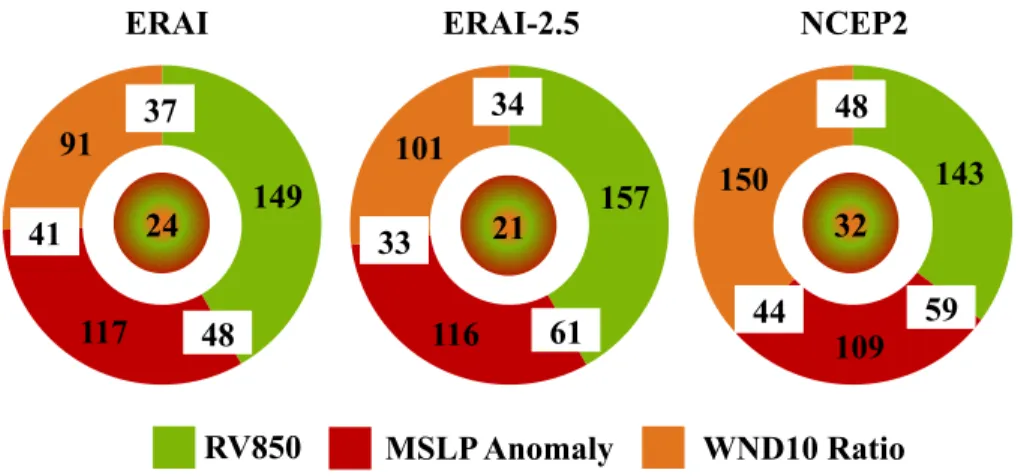
Fig. 4 presents for each reanalysis datasets the number of events detected with each of the variables, the number of common events to pair-wise variables and the number of events in the final set (i.e. events common to the three variables).

The number of events common to the three variables is always reduced compared to the number for individual variables: 24 events with ERAI, 21 with ERAI-2.5 and 33 with

25

(15)

NHESSD

1, 4257–4285, 2013

Title Page

Tables Figures

◭ ◮

Back Close

Full Screen / Esc

Discussion

P

a

per

|

Dis

cussion

P

a

per

|

Discussion

P

a

per

|

Discussio

n

P

a

per

|

relative vorticity and the anomaly of MSLP are lower than the 95th percentile. ERAI and ERAI-2.5 share 15 common final events, while ERAI-2.5 and NCEP2 have 16 (not shown in the figure). For each reanalysis dataset, the final set of events can thus be divided in two groups: one group with events common to the three reanalysis datasets (including the reference storms) and another one with events specific to the reanalysis

5

dataset.

For each dataset, we are therefore able to isolate a small group of events sharing a similar meteorological surface-signature with the ten reference storms, with no need to modify the parameters of the method. The use of percentile-based thresholds leads to the detection of a similar number of extreme events with different resolutions; these

10

events are however generally not the same or ranked di_fferently, with the exception of the ones obtained from the MSLP anomaly. The multi-variables approach enables in each case to further restrict the number of selected events (roughly by a factor of 4), while retaining all the major ones.

5 Conclusions

15

The methodology presented in this paper enables a reliable detection of events with high damage potential, easily adaptable to di_fferent datasets or model outputs. Its ro-bustness comes from two main factors. The use of thresholds based on percentiles of the distribution of the variables as only parameters ensures the adaptability to different datasets, especially with varying resolutions. More originally, we showed that an

ap-20

proach based on several variables of di_fferent scales was more e_fficient than trying to select extreme events in a single variable. Indeed, when only one variable is consid-ered, a number of minor events need to be retained in order to get all the known major ones (e.g. the ten storms since 1987), thereby weakening the selectivity. Moreover, these weaker events largely di_ffer according to the variable considered or the

reanal-25

(16)

NHESSD

1, 4257–4285, 2013

Title Page

Tables Figures

◭ ◮

Back Close

Full Screen / Esc

Discussion

P

a

per

|

Dis

cussion

P

a

per

|

Discussion

P

a

per

|

Discussio

n

P

a

per

|

events that have a strong signature in several variables at once therefore proved to be a simple but e_fficient filter.

The method’s novelty lies in its ability to target extreme events having a great im-pact on insurance policies while using exclusively meteorological variables. Previous research on ETCs usually consists either in analysis of their physical properties or in

5

loss models applied to the European insurance market, each of these analyses ad-dressing specific questions. Our method instead uses a simple combination of relevant physical parameters to detect potential high-loss events. This will be of particular inter-est for the construction of event catalogues in current and future climates, contributing to improve the monitoring of European winter windstorms, by the insurance companies

10

for example.

The next step of the project will be to apply the methodology to the outputs of the CMIP5 model ensemble in order to create catalogues of extra tropical storms in the North Atlantic–Western Europe region and to compare the events detected in historical and scenario runs.

15

Acknowledgements. Madeleine-Sophie Deroche is grateful to the AXA Research Fund for the PhD grant that supports the research for this paper. The authors wish to express their gratitude to Gwendal Rivi `ere as well as to previous reviewers for their helpful comments.

The publication of this article is financed by CNRS-INSU.

20

References

(17)

NHESSD

1, 4257–4285, 2013

Title Page

Tables Figures

◭ ◮

Back Close

Full Screen / Esc

Discussion

P

a

per

|

Dis

cussion

P

a

per

|

Discussion

P

a

per

|

Discussio

n

P

a

per

|

Campins, J., Genov ´es, A., Picornell, M. A., and Jans `a, A.: Climatology of Mediterranean cy-clones using the ERA-40 dataset, Int. J. Climatol., 31, 1596–1614, 2011.

Dee, D. P., Uppala, S. M., Simmons, A. J., Berrisford, P., Poli, P., Kobayashi, S., Andrae, U., Balmaseda, M. A., Balsamo, G., Bauer, P., Bechtold, P., Beljaars, A. C. M., Van de Berg, L., Bidlot, J., Bormann, N., Delsol, C., Dragani, R., Fuentes, M., Geer, A. J., Haimberger, L.,

5

Healy, S. B., Hersbach, H., H ólm, E. V., Isaksen, L., K ˚allberg, P., K öhler, M., Matricardi, M., McNally, A. P., Monge-Sanz, B. M., Morcrette, J.-J., Park, B.-K., Peubey, C., De Rosnay, P., Tavolato, C., Th épaut, J.-N., and Vitart, F.: The ERA-interim reanalysis: configuration and performance of the data assimilation system, Q. J. Roy. Meteor. Soc., 137, 553–597, 2011. Della-Marta, P. M., Mathis, H., Frei, C., Liniger, M. A., Kleinn, J., and Appenzeller, C.: The return

10

period of wind storms over europe, Int. J. Climatol., 29, 437–459, 2009.

Donat, M. G., Leckebusch, G. C., Wild, S., and Ulbrich, U.: Future changes in European win-ter storm losses and extreme wind speeds inferred from GCM and RCM multi-model sim-ulations, Nat. Hazards Earth Syst. Sci., 11, 1351–1370, doi:10.5194/nhess-11-1351-2011, 2011.

15

Feldstein, S. B.: The timescale, power spectra, and climate noise properties of teleconnection patterns, J. Climate, 13, 4430–4440, 2000.

Gulev, S. K., Zolina, O., and Grigoriev, S.: Extratropical cyclone variability in the Northern Hemi-sphere winter from the NCEP/NCAR reanalysis Data, Clim. Dynam., 17, 795–809, 2001. Hanley, J. and Caballero, R.: Objective identification and tracking of multicentre cyclones in the

20

ERA-interim reanalysis dataset, Q. J. Roy. Meteor. Soc., 138, 612–625, 2012.

Hodges, K. I.: Spherical nonparametric estimators applied to the UGAMP model integration for AMIP, Mon. Weather Rev., 124, 2914–2932, 1996.

Hodges, K. I., Lee, R. W., and Bengtsson, L.: A comparison of extratropical cyclones in recent reanalyses ERA-interim, NASA MERRA, NCEP CFSR, and JRA-25, J. Climate, 24, 4888–

25

4906, 2011.

Hoskins, B. J. and Hodges, K. I.: New perspectives on the Northern Hemisphere winter storm tracks, J. Atmos. Sci., 59, 1041–1061, 2002.

Kanamitsu, M., Ebisuzaki, W., Woollen, J., Yang, S.-K., Hnilo, J. J., Fiorino, M., and Potter, G. L.: NCEP–DOE AMIP-II reanalysis (R-2), B. Am. Meteorol. Soc., 83, 1631–1643, 2002.

30

(18)

NHESSD

1, 4257–4285, 2013

Title Page

Tables Figures

◭ ◮

Back Close

Full Screen / Esc

Discussion

P

a

per

|

Dis

cussion

P

a

per

|

Discussion

P

a

per

|

Discussio

n

P

a

per

|

Leckebusch, G. C., Ulbrich, U., Fr ¨ohlich, L., and Pinto, J. G.: Property loss potentials for European midlatitude storms in a changing climate, Geophys. Res. Lett., 34, L05703, doi:10.1029/2006GL027663, 2007.

Leckebusch, G. C., Renggli, D., and Ulbrich, U.: Development and application of an objective storm severity measure for the northeast Atlantic region, Meteorol. Z., 17, 575–587, 2008.

5

Lionello, P., Dalan, F., and Elvini, E.: Cyclones in the Mediterranean region: the present and the

doubled CO₂climate scenarios, Clim. Res., 22, 147–159, 2002.

Murray, R. and Simmonds, I.: A numerical scheme for tracking cyclone centres from digital data. I. Development and operation of the scheme, Aust. Meteorol. Mag., 39, 155–166, 1991. Neu, U., Akperov, M. G., Bellenbaum, N., Benestad, R., Blender, R., Caballero, R., Co- cozza,

10

A., Dacre, H. F., Feng, Y., Fraedrich, K., Grieger, J., Gulev, S., Hanley, J., Hewson, T., Inatsu, M., Keay, K., Kew, S. F., Kindem, I., Leckebusch, G. C., Liberato, M. L. R., Lionello, P., Mokhov, I. I., Pinto, J. G., Raible, C. C., Reale, M., Rudeva, I., Schuster, M., Simmonds, I., Sinclair, M., Sprenger, M., Tilinina, N. D., Trigo, I. F., Ulbrich, S., Ulbrich, U., Wang, X. L.,

and Wernli, H.: IMILAST – a community effort to intercompare extratropical cyclone detection

15

and tracking algorithms: assessing method-related uncertainties, B. Am. Meteorol. Soc., 94, 529–547, doi:10.1175/BAMS-D-11-00154.1, 2013

Nissen, K. M., Leckebusch, G. C., Pinto, J. G., Renggli, D., Ulbrich, S., and Ulbrich, U.: Cyclones causing wind storms in the Mediterranean: characteristics, trends and links to large-scale patterns, Nat. Hazards Earth Syst. Sci., 10, 1379–1391, doi:10.5194/nhess-10-1379-2010,

20

2010.

Pinto, J. G., Spangehl, T., Ulbrich, U., and Speth, P.: Sensitivities of a cyclone detection and tracking algorithm: individual tracks and climatology, Meteorol. Z., 14, 823–838, 2005. Pinto, J. G., Fr ¨ohlich, E. L., Leckebusch, G. C., and Ulbrich, U.: Changing European storm

loss potentials under modified climate conditions according to ensemble simulations of the

25

ECHAM5/MPI-OM1 GCM, Nat. Hazards Earth Syst. Sci., 7, 165–175, doi:10.5194/nhess-7-165-2007, 2007.

Pinto, J., Karremann, M., Born, K., Della-Marta, P., and Klawa, M.: Loss potentials associated with European windstorms under future climate conditions, Clim. Res., 54, 1–20, 2012. Rivi `ere, G. and Joly, A.: Role of the low-frequency deformation field on the explosive growth

30

(19)

NHESSD

1, 4257–4285, 2013

Title Page

Tables Figures

◭ ◮

Back Close

Full Screen / Esc

Discussion

P

a

per

|

Dis

cussion

P

a

per

|

Discussion

P

a

per

|

Discussio

n

P

a

per

|

Sinclair, M. R.: Objective identification of cyclones and their circulation intensity, and climatol-ogy, Weather Forecast., 12, 595–612, 1997.

(20)

NHESSD

1, 4257–4285, 2013

Title Page

Tables Figures

◭ ◮

Back Close

Full Screen / Esc

Discussion

P

a

per

|

Dis

cussion

P

a

per

|

Discussion

P

a

per

|

Discussio

n

P

a

per

|

Table 1.List of the European winter windstorm that caused more than 1 thousand million US Dollar over the last 30 yr. In bold are the ten reference storms used in our study (Source: Com-piled by Earth Policy Institute from Munich Re, “Natural Disasters: Billion-$ Insurance Losses”, in Louis Perroy, “Impacts of Climate Change on Financial Institutions’ Medium to Long Term As-sets and Liabilities”, presented to the Staple Inn Actuarial Society, 14 June 2005; Munich Re, Topics Geo: Natural Catastrophes 2004, 2005, 2006, 2007, 2008, and 2009, Munich: 2005, 2006, 2007, 2008, 2009, and 2010).

Year Winter storm name Insured Losses Economic Losses

US$ m, original values

Oct 1987 87J 3100 3700

Jan 1990 Daria 5100 6800

Feb 1990 Herta 1300 1950

Feb 1990 Vivian 2100 3200

Feb 1990 Wiebke 1300 2250

Dec 1999 Anatol 2350 2900

Dec 1999 Lothar 5900 11 500

Dec 1999 Martin 2500 4100

Oct 2002 Jeanett 1500 2300

Jan 2005 Erwin 2500 5800

Jan 2007 Kyrill 5800 10 000

Feb 2008 Emma 1500 2000

Jan 2009 Klaus 3000 5100

(21)

NHESSD

1, 4257–4285, 2013

Title Page

Tables Figures

◭ ◮

Back Close

Full Screen / Esc

Discussion

P

a

per

|

Dis

cussion

P

a

per

|

Discussion

P

a

per

|

Discussio

n

P

a

per

|

Table 2.The ten reference storm events are ranked: in the second row according the insured losses (Munich Re), from the third to the fifth column according to the maximum value they reach as ERA Interim events of relative vorticity at 850 hPa (RV850), anomaly of the mean sea-level pressure (MSLP ANOM) and 10 m wind speed ratio (WND10 RATIO). For example, with the relative vorticity at 850 hPa (RV850), we detect 149 events that we ranked according the maximum of RV850 reached during their period they are detected over the window. Here we present the rank for the ten reference storms only.

Event Munich Re RV850 MSLP ANOM WND10 RATIO

Lothar 1 32 57 2

Kyrill 2 43 15 30

Daria 3 19 12 25

87J 4 2 9 11

Xynthia 5 22 49 28

Klaus 6 51 59 1

Martin 7 6 6 3

Erwin 7 39 38 8

Anatol 8 1 7 19

(22)

NHESSD

1, 4257–4285, 2013

Title Page

Tables Figures

◭ ◮

Back Close

Full Screen / Esc

Discussion

P

a

per

|

Dis

cussion

P

a

per

|

Discussion

P

a

per

|

Discussio

n

P

a

per

|

Table A1.Table of variables and acronyms.

Variables:

MSLP: Mean Sea Level Pressure

MSLP8 days: Running Average over eight days of the mean sea level pressure MSLPanom: Mean sea level pressure anomaly

RV850: Relative Vorticity at 850 hPa (hectoPascal) WND10: 10 m wind speed

WND10₉₈: 98th percentile of the 10 m wind speed, computed for each grid point over the whole given period WND10ratio: Ratio of the 10 m wind speed over its 98th percentile

Datasets:

ERAI: ERA Interim

ERAI-2.5: ERA Interim downgraded at 2.5◦ NCEP2: NCEP-DOE Reanalysis 2

Other:

CMIP5: Coupled Model Intercomparison Project Phase 5

ECMWF: European Centre for Medium-Range Weather Forecasts ETC: Extra-Tropical Cyclone

(23)

NHESSD

1, 4257–4285, 2013

Title Page

Tables Figures

◭ ◮

Back Close

Full Screen / Esc

Discussion

P

a

per

|

Dis

cussion

P

a

per

|

Discussion

P

a

per

|

Discussio

n

P

a

per

|

Fig. 1. Maps for the three variables’ fields at the time of Lothar (from 26 December 1999, 00:00 UTC to 26 December 1999, 12:00 UTC) in ERA Interim: first row, relative vorticity at

850 hPa (1 s−1_{); second row the mean sea-level pressure anomaly (hPa); last row, the 10 m}

(24)

NHESSD

1, 4257–4285, 2013

Title Page

Tables Figures

◭ ◮

Back Close

Full Screen / Esc

Discussion

P

a

per

|

Dis

cussion

P

a

per

|

Discussion

P

a

per

|

Discussio

n

P

a

per

|

87/8889/9091/9293/9495/9697/9899/0001/0203/0405/0607/0809/10 0

1 2 3 4 5 6

x1.e04

October−March 1987−2010 RV850 (1/s)

87/8889/9091/9293/9495/9697/9899/0001/0203/0405/0607/0809/10 −15

−5 5 15 25 35 45

October−March 1987−2010 MSLP Anomaly (hPa)

87/8889/9091/9293/9495/9697/9899/0001/0203/0405/0607/0809/10 0

0.5 1 1.5 2 2.5

October−March 1987−2010 WND10 Ratio

87J

DariaVivianAnatolLotharMartinErwinKyrillKlaus_Xynthia 1

2 3 4 5 6

RV850 (1/s) x1.e04

87J

20 25 30 35 40 45

MSLP Anomaly (hPa)

87J

1.5 2 2.5

WND10 Ratio

Fig. 2.The first row shows the time series of the detected maxima of each variable over the time period (six-hourly time steps over October–March from 1987 to 2010, i.e. 16 768 maxima) and geographical window. The horizontal lines are the 95th (dashed red line) and 98th (blue line) quantiles of the distribution of the maxima of each variable. The second row represents the values of the maxima of each variable at the time of occurrence of the ten reference storms.

(25)

NHESSD

1, 4257–4285, 2013

Title Page

Tables Figures

◭ ◮

Back Close

Full Screen / Esc

Discussion

P

a

per

|

Dis

cussion

P

a

per

|

Discussion

P

a

per

|

Discussio

n

P

a

per

|

RV850 MSLP

ANOM

WND10 RATIO

SET 1 SET 2 SET 3

4) LOOKING FOR COMMON EVENTS

FINAL SET

1)! DETECTION

(maxima threshold: 95th_perc.) 2)! TRACKING

(eastward shift & distance < 900 km) 3)! SELECTION

(maximum event threshold: 98th_perc.)

(26)

NHESSD

1, 4257–4285, 2013

Title Page

Tables Figures

◭ ◮

Back Close

Full Screen / Esc

Discussion

P

a

per

|

Dis

cussion

P

a

per

|

Discussion

P

a

per

|

Discussio

n

P

a

per

|

157

116 101

34

61 33 21 149

117 91

37

48 41 24

143

109 150

59 44

48

32

ERAI ERAI-2.5 NCEP2

RV850 MSLP Anomaly WND10 Ratio

(27)

NHESSD

1, 4257–4285, 2013

Title Page

Tables Figures

◭ ◮

Back Close

Full Screen / Esc

Discussion

P

a

per

|

Dis

cussion

P

a

per

|

Discussion

P

a

per

|

Discussio

n

P

a

per

|

0 1 2 3 4 5 6 0

0.1 0.2 0.3 0.4 0.5 0.6

RV850 (1/s)

Density

x1.e−04 ERAI ERAI−2.5 NCEP2

−20 0 20 40 60 0

0.1 0.2 0.3 0.4 0.5 0.6

MSLP Anomaly (hPa)

Density

ERAI ERAI−2.5 NCEP2

0.5 1 1.5 2 0

0.1 0.2 0.3 0.4 0.5 0.6

WND10 Ratio

Density

ERAI ERAI−2.5 NCEP2

(28)

NHESSD

1, 4257–4285, 2013

Title Page

Tables Figures

◭ ◮

Back Close

Full Screen / Esc

Discussion

P

a

per

|

Dis

cussion

P

a

per

|

Discussion

P

a

per

|

Discussio

n

P

a

per

|

RV850

MSLP Anomaly

WND10 Ratio

0

20

40

60

80

100 ERAI−ERAI2.5

ERAI2.5−NCEP2

(29)

NHESSD

1, 4257–4285, 2013

Title Page

Tables Figures

◭ ◮

Back Close

Full Screen / Esc

Discussion

P

a

per

|

Dis

cussion

P

a

per

|

Discussion

P

a

per

|

Discussio

n

P

a

per

|

117

116 109

107 100

149

157 143

104 71

91

101 150

62

67

RV850 MSLP Anomaly WND10 Ratio

ERAI ERAI-2.5 NCEP2

a)

b) RV850 MSLP Anomaly WND10 Ratio

Anatol 87J

MartinDariaXynthiaLotharErwinKyrillKlausVivian

0 70 140

Rank of ev

ents

VivianMartinAnatol 87J

DariaKyrillErwin_XynthiaLotharKlaus

0 55 110

Rank of ev

ents

Klaus_Lothar_MartinErwin87JAnatolDariaXynthiaK yrill

Vivian

0 40 80

Rank of ev

ents

Fig. 7. (a): per variable, number of events detected within each reanalysis dataset and number of common events between ERAI (dark blue squares) and ERAI2.5 (light blue diamonds), be-tween ERAI-2.5 and NCEP2 (black triangles). For example, with the relative vorticity (RV850), 149 events are detected within ERAI, 157 within ERAI-2.5 and 143 within NCEP2. 104 events are common to ERAI and ERAI-2.5 (i.e. 104 events have been detected simultaneously in ERAI and ERAI-2.5 during at least one time step) and 69 are common to ERAI-2.5 and NCEP2.