Abstract— This paper presents an evaluation of the phase shifting excitation and load effects in a Transmission Line Exciting Chamber. This chamber is suggested as an alternative for immunity tests because of the restrictions related to canonical chambers. Here, two methods are used to calculate the E-field: a semi-analytic approach and a numerical one. The semi-analytic method is based on the modal expansion while a software is used for numerical simulations. The results regarding the E-field profile and the related statistical indexes of merit are presented and used to evaluate the chamber performances. Experiments were also conducted in order to evaluate the chamber.
Index Terms— Reverberation chamber, random excitations and loads,
transmission lines.
I. INTRODUCTION
Canonical chambers - like Reverberation Chambers (RC) and TEM chambers - are generally used for electromagnetic immunity testing despite their particular operational restrictions. RCs using mechanical paddles or frequency stirring provide a statistical E-field uniformity in all the directions inside the working volume [1], [2]. Nevertheless, the operation frequency of RCs is inversely proportional to the chamber dimensions and it is a constraint for low frequency tests. The international standards recommend the RC configuration for immunity tests over 80 MHz frequencies [2], [3].
Among the first published works concerning RCs we can mention [4],[5], [6], and [7]. These authors have proposed two different approaches in order to change the boundary conditions inside the chamber: constant rotating paddles and step-by-step paddles. On the contrary, TEM chambers operate in the low frequency range. Introducing a stripline inside the chamber, a deterministic E-field uniformity is reached over a working area parallel to the plate, but not for all the polarizations in the chamber volume. Some early works with TEM cells were proposed by [8]. The performances of the TEM cells were extendedinall polarizations using three orthogonal striplines [9].
An overview on the usual electromagnetic compatibility test methods is presented in [10], and herein a comprehensive list of references on these methods can be founded.
Recently, an alternative concept called Transmission Line Exciting Chamber (TLEC) has been
A Load Effect Evaluation of a Transmission
Line Exciting Chamber
Mario. A. Santos Jr.(1), Damien Voyer(2), Ronan Perrussel(2), Djonny Weinzierl(3), Carlos. A. F. Sartori(1), Laurent Krähenbühl(2), Christian Vollaire(2), José R. Cardoso(1)
(1)Lab. de Eletromagnetismo Aplicado LMAG/PEA/EPUSP. 05508-900. São Paulo-SP, Brazil
(2)
Lab. Ampère (CNRS UMR5005), Université de Lyon, Ecole Centrale de Lyon, 69134, Ecully Cedex - France
(3)
proposed, based on a phase shifting excitation of several transmission lines (TL). For the sake of illustration, a structure constituted of three conductors with a phase shifting excitation has been investigated in [11], [12].
Basically, a chamber excited by several TLs presents several TEM modes inside the closed metallic cavity. The resulting standing waves depend on the position of the TLs, on the amplitude and phase of the excitations, and on the loading at the end of the TLs. Those parameters are important in the search for a suitable chamber working volume; they can be modified electronically, resulting in a random standing wave profile. Based on this, the performances of the TLEC can be improved to satisfy the pre-defined uniformity criteria within a wide frequency range, even at frequencies lower than 80 MHz. In this work, we present semi-analytical and numerical approaches as well as an experimental setup for evaluating the performance of a TLEC.
II. SEMI-ANALYTIC APPROACH
A. Analytic expression for a TL
Consider the TL geometry given by Fig.1. When one analyzes the E-field of a single TEM mode, the dependence on the longitudinal direction z can be decoupled from the dependence on the transverse x and y directions. Indeed, the propagation, which exists for any frequency, can be described by a function e-jk0z when an incident wave is considered; k0 is the wave number in the vacuum. The problem of the impact of possible reflections at the end of the TL will be addressed further in subsection II.C.
Y
Z
a x0
l
l
Central conductor
External walls of the chamber
X
l1
l2
Fig. 1. Geometry of a TL in the transverse plane
(
)
(
)
(
)
∑
+∞ = < + > − × = 1 m 2 m 2 1 m 1 0 X TEM 0 y l y a m sh 0 y l y a m sh x a m cos a 2 y , x E π α π α π η , (1) ( ) ( ) ( )∑
+∞ = < + > − × = 1 m 2 m 2 1 m 1 0 Y TEM 0 y l y a m ch 0 y l y a m ch x a m sin a 2 y , x E π α π α π η , (2) with 2 1 1 1 2 m m th l aJ m m
ch l
a
m m
th l th l
a a π π α π π = + , 1 2 2 1 2 m m th l a Jm m ch l a m m
th l th l
a a π π α π π = − + , (3)
where η0 is the vacuum wave impedance and Jm the harmonic coefficients related to the current density on the central conductor. Assuming that the conductor is an infinitely thin wire along z axis, one finds:
= 0 0
m x a m sin a 2 I J π
.
(4)B. Several lines and Phase Shifting
When several TLs are ended with the same load, the E-field can still be written using the separation of variables in the transverse plane and in the longitudinal direction. The problem can then be treated by superposition:
(
)
=∑
(
)
i TEM i iTOT x,y IE x,y E
,
(5)
where i T ΕM
Ε is the E-field due to the ith TL for a current of amplitude unitary and Ii represents the
applied excitation current. The phase shifting between the TLs has then an effect on the repartition of the E-field in the transverse plane.
C. Load Shifting
The load at the end of the TLs introduces a reflection coefficient Γ that affects the longitudinal repartition of the field:
(
)
(
) (
jkz jkz)
TOT x,y e 0 e 0 E z , y , x
E = × − +Γ +
.
(6)Concerning the stripline used in canonical TEM chambers, the design of the TL is such that there is no reflection. Then the magnitude of the field is uniform in z direction. Using a TL with a thin wire, there is a discontinuity at the end of the line and it is difficult to match the line with the suitable load; then |Γ | ≠ 0 and a stationary wave is expected.
(
)
(
) (
)
(
)
j /20 TOT z jk j z jk TOT e 2 z k cos y , x E 2 e e e y , x E z , y , x
E 0 0
φ φ φ + × = + × = − +
.
(7)The phase shifting φ/2 in the cosinus function shows that the maxima and minima of the E-field in z direction move with φ. When the phase varies linearly between 0 and 2π, the time-average effect can be calculated as follows:
(
)
(
)
d 4 E(
x,y)
2 1 z , y , x E z , y , x E TOT 2 0
average π φ π
π
= =
∫
.
(8)
The average E-field is no more dependent on z direction. Thus, it is possible to homogenize the field in z direction even if the TL is unmatched.
III. NUMERICAL APPROACH
Numerical evaluation was performed with the Finite Integration Technique by using the commercial software CST-MWS ® [16]. The interest is that this approach is more realistic than the semi-analytic one since it takes into account the connection of the TLs outside the chamber; those details introduce discontinuities that can have an impact on the distribution of the E-field. A 3D TLEC model is built considering PEC walls and PEC TLs. The loads are set using ports defined at the end of the TLs while the phase shifting excitation is implemented in a post-processing treatment.
A procedure applying Matlab® Activex commands was performed in order to set up the calculation parameters at CST-MWS® and to perform the indexes of merit calculation discussed in the following section.
IV. INDEXES OF MERIT
The uniformity of the field is evaluated using the indexes of merit defined in [17]. Due to the phase and load shifting, the E-field considered at any point of the chamber is the average field Eaverage in time. Considering a spatial point k in the chamber, one finds for the x polarization of the average field:
(
)
( )
[ ]∫
∏
+ = + = 1 M 2 , 0 M 1 i i 1 M M 1 k x k x _average d d
2 , , , E E π ϕ φ π ϕ ϕ
φ
,
(9) with k
( )
x
E the module of E-field in the point k and x direction, φ the phase of Γ, ϕi the phase of the current Ii in the i
th
TL and M the number of TLs. Numerically, the integral is computed using a finite number of phases.
Then the mean field Ex and the standard deviation σx in the spatial domain can be computed from the average field given in (10):
∑
= = N 1 k k x _ averagex N E
1
E
,
(
)
∑
= − − = N 1 k 2 x k x _ averagex N 1 E E
1
σ
,
(10)
The normalized standard deviation in dB σˆx in x direction is defined by:
10
ˆ 20 log x x x
x E
E
σ
σ = +
.
(11)
The index in y directions is calculated similarly.
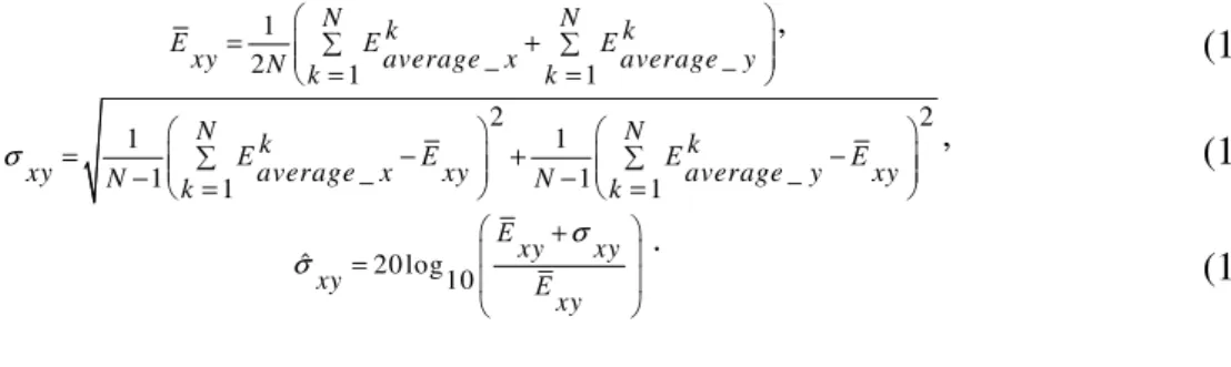
In the same way, an index can be defined to take into account both components of the E-field in the transverse plane:
1
2 1 1
N k N k
Εxy Εaverage _ x Εaverage _ y
N k k
= ∑ + ∑
= =
,
(12)
2 2
1 1
_ _
1 1 1 1
N k N k
Ε Ε Ε Ε
xy N average x xy N average y xy
k k
σ = ∑ − + ∑ −
− = − =
,
(13)
ˆ 20 log 10
Εxy xy
xy Ε
xy
σ σ
+
=
.
(14)
V. SIMULATION RESULTS
A TLEC with dimensions of 0.6m×0.6m×1.2m(see Fig.2) has been considered; the volume under evaluation (WV) is a parallelepiped of dimensions 0.3m×0.3m×0.6m centered at the middle of the chamber. Besides that, the area under evaluation (WA) is a square of dimensions 0.3m x 0.3mat the center of WV. All the simulations were performed for a frequency of 80 MHz.
Fig. 2. WV and WA definitions in the TLEC
A. Semi-analytical results
The semi-analytical approach has been applied in the transverse plane {x, y} since the variation of E-field in z direction can be canceled using a suitable load shifting. The study concerns the influence of the phase shifting when several TLs are considered.
(a)
(b)
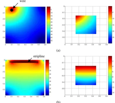
Fig. 3. Distribution of the normalized E-field in the transverse plane inside the chamber (on the left) and inside the WA (on the right) in dB: (a) TL with a thin wire conductor (b) stripline used in canonical TEM chambers
It appears that none of the TL induces a uniform field; however the variation of the E-field magnitude inside the working area is greater in the case of the TL with a thin wire conductor (30 dB) compared to the stripline (15 dB). This result should prove that the stripline is a better candidate.
However when one takes into account some practical considerations in the realization of the lines, the TL with wire conductor remains an attractive solution. Then, to improve the E-field uniformity, a solution consists in using several TLs. Fig.4 illustrates the situation where currents with I1=I2=1 and
I3=I4=-1 flow along the 4 TLs inside the TLEC; as one can see, it still remains minima and maxima of
the E-field.
Basically, it is possible to move the minima and maxima of the total E-field inside the working area by changing the excitations I1, I2, I3 and I4 of the 4 TLs. For sake of illustration, two examples are given Fig.5.
I1 I2
I3 I4
Fig. 4. Distribution of the normalized E-field inside the chamber with 4TL excited by I1=I2=1 and I3=I4=-1 wire
(a) (b)
Fig.5. Distribution of the normalized E-field inside the working area for different excitations: (a) I1=I2=1 I3=j I4=-1 (b) I1=1 I2=j I3=-j I4=-1/4
A better uniformity of the E-field can then be achieved by introducing a random variation of the excitations. The excitation shifting can be applied to the amplitude or to the phase of the different currents. Fig.6 shows that the effect on the average E-field is the same whenever the phase or the amplitude is supposed to be random. However, due to practical considerations, the phase shifting technique should be retained here. The variation of the E-field magnitude inside the working area is less important in the case of the 4 TLs with phase shifting (10 dB) compared to the stripline (15 dB) studied previously (see Fig.4b).
Fig. 6. Distribution of the mean normalized E-field inside the working area with an amplitude shifting (on the left) or a phase shifting (on the right)
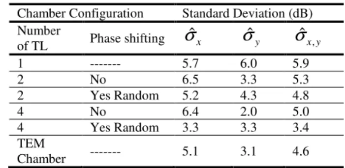
Results in terms of indexes of merit are reported in Table I. It appears that the number of TLs is an important parameter: the standard deviation decreases of 3 dB when 4 TLs are introduced instead of 2 TLs. Moreover, the phase shifting improves of 0.5 dBto3 dB the performances of the chamber.
TABLE I. STANDARD DEVIATIONS FOR SEMI-ANALYTICAL APPROACH
Chamber Configuration Standard Deviation (dB) Number
of TL Phase shifting
σ
ˆ
xσ
ˆyσ
ˆx y,1 --- 5.7 6.0 5.9
2 No 6.5 3.3 5.3
2 Yes Random 5.2 4.3 4.8
4 No 6.4 2.0 5.0
4 Yes Random 3.3 3.3 3.4
TEM
Chamber --- 5.1 3.1 4.6
B. Numerical results
terminated by a 50 Ω load (the characteristic impedance of the TLs is 250 Ω, measured with a Vectorial Network Analyser at 100MHz frequency). As one can see, the results in the WA are close to the ones given in Table I: for example the difference is about 0.5 dB in the case of 4 TLs with random phase shifting. However, there is a difference with the results when the WV is considered: this is due to the standing wave that appears because the TLs are unmatched. However, the difference never exceeds 1 dB because the dimension of the WV in z direction (0.6 m) is not large compared to the wavelength (3.75 m at 80 MHz).
TABLE II. STANDARD DEVIATIONS FOR NUMERICAL APPROACH (LOAD 50Ω)
Chamber Configuration Standard Deviation (dB) Number
of TL
Phase shifting
Working
region σˆx σˆy σˆx y,
1 ---- WA 6.1 6.1 6.1
WV 7.3 7.3 7.3
2 No WA 7.7 3.6 4.9
WV 7.8 3.8 5.1
2 Yes
Random
WA 5.9 4.0 4.8
WV 6.0 4.2 5.0
4 No WA 6.5 2.7 3.8
WV 6.6 2.9 4.0
4 Yes
Random
WA 3.9 3.9 3.9
WV 4.0 4.1 4.1
The performances in the WV can be improved by a load shifting. The effect of changing the load is presented in Fig.7. It appears that the maximum of E-field moves between a load of -j500 Ω and +j500 Ω. Considering that the characteristic impedance of the TLs is 250 Ω, one finds that the reflection coefficient Γ is respectively e-j0.93and e+j0.93; goingback to equation (7), one expects that the minimum of E-field moves of 0.93÷ k0 = 0.55 m between both loads. This result is illustrated by the
simulations reported in Fig.8 (remind that the dimension of the chamber in z direction is 1.2 m, that is to say approximately 2×0.55 m).
(a) (b)
Fig. 7. Distribution of the E-field modulus inside the chamber for differents loads at 0.3m plane (a) -j500 Ω load (b) +j500 Ω
load
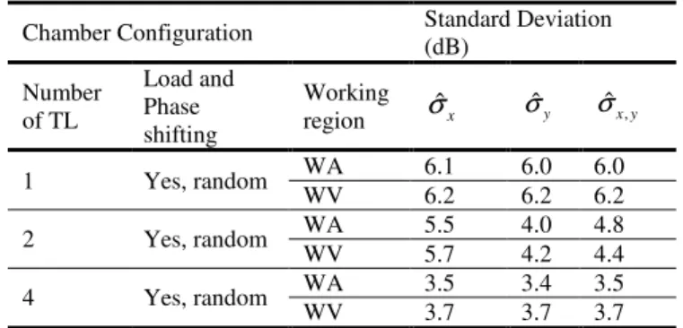
difference is 0.1 to 0.2 dB in the case of a single TL.
TABLE III. STANDARD DEVIATIONS FOR NUMERICAL APPROACH (LOAD SHIFTING)
Chamber Configuration Standard Deviation (dB)
Number of TL
Load and Phase shifting
Working
region σˆx σˆy σˆx y,
1 Yes, random WA 6.1 6.0 6.0
WV 6.2 6.2 6.2
2 Yes, random WA 5.5 4.0 4.8
WV 5.7 4.2 4.4
4 Yes, random WA 3.5 3.4 3.5
WV 3.7 3.7 3.7
VI. EXPERIMENTAL PROCEDURE AND RESULTS
In order to evaluate the chamber performance, an experimental setup has also been carried out. Basically, the results related to the field profile, and the related effects of the phase and the load-shifting have been obtained.
Fig. 8 presents the chamber prototype, which was built with galvanized steel ASTM 1020. It is composed of two asymmetric cooper transmission lines ended by N type connectors. The transmission lines are positioned at x1=0.10m, y1=0.45m and x2=0.50m, y=0.50m, they were built in asymmetric positions to avoid deep nulls in E-field when the terminals are excited in 180 degrees shift (as proposed by [11]). This configuration was chosen in order to improve the chamber performance.
Fig. 8. Internal view of the TLEC prototype
A. Load shifting test
Phase-Shifter Standard load 50Ω
TLEC Out connector
In Vcc Control
Fig. 9. Experimental setup - detail of phase-shifter as TLEC load.
The load shifting has been experimented using a phase-shifter and an open termination for the frequency range of 100MHz-190MHz. Fig. 10 shows the impedance seen at the input of the TL; note that the measured reflection coefficient is not exactly the reflection coefficient Γ discussed in section II.C. However, it appears that the impedance changes when different voltage values are applied to the phase-shifter control terminal. Since the phase shifter can be electronically controlled, a random load shifting can thus be obtained in order to generate a better uniformity of the E-field in the TLEC.
Fig. 11 shows that the S-parameters measured at the input of the TLs are in agreement with those simulated with CST-MWS ®. Note that there is a resonance at 125 MHz due the apparition of a cavity mode ; the peak value that is not exactly the same between simulation and measurement because of the losses that are not taken into account in the modeling.
Comparação de Parâmetros S11 e S22 - Medidos e Simulados
S11 Medido
S11 Simulado
S22 Medido S22 Simulado
S (dB)
Freqüência (MHz)
S11 and S22 with 50
Ω
load
S11 measured
S11 simulated
S22 measured
S22 simulated
Comparação de Parâmetros S11 e S22 - Medidos e Simulados
S11 Medido
S11 Simulado
S22 Medido S22 Simulado
S (dB)
Freqüência (MHz)
S11 and S22 with 50
Ω
load
Comparação de Parâmetros S11 e S22 - Medidos e Simulados
S11 Medido
S11 Simulado
S22 Medido S22 Simulado
S (dB)
Freqüência (MHz)
S11 and S22 with 50
Ω
load
S11 measured
S11 simulated
S22 measured
S22 simulated
Fig. 11. TLEC Measured and Simulated S11 and S22 for 50Ω load.
B. E-field measurements
Measurements of the E-field have been made at chamber center (0.3 m; 0.3 m; 0.6 m), by using an isotropic probe Holaday model HI422, positioned by a PVC tube, as shown at Fig. 12.
Fig. 12. Photo of the TLEC showing the details of the isotropic field probe.
Fig. 13. Comparison between experimental and simulated field at P(0.3m, 0.3m, 0.6m), for the 50 Ohm load.
The same experiment has been carried out with an open load, see Fig. 14. One can observe that the results between measurement and simulation are not exactly in agreement. This is due to the presence of the connectors at the end of the TL (see Fig. 9) that is not taken into account in the numerical modeling. Indeed, connectors introduce a short transmission line that can change the impedance seen by the open load.
Fig. 14. Comparison between experimental and simulated E-field at P(0.3m, 0.3m, 0.6m), for the open load.
one in literature in order to characterize devices in the high frequency range. This is why we have only reported S parameters measurements which are better suited to these applications as reported in section A.
CONCLUSION
Semi-analytic, numerical simulation and experimental results have been provided in order to make full relationship between theory and real measurements for the TLEC characterization; all these results are in good agreement when considering the limitations of each method.
Then, when a TLEC is well designed and operated, it can reach and overcome the uniformity standards stated to canonical chambers.
ACKNOWLEDGMENT
This work was partially supported by Capes-Cofecub (07/0568), FAPESP (2007/51192-6) and Brazilian Navy.
REFERENCES
[1] D. Hill, “Electronic mode stirring for reverberation chambers”, IEEE Transactions on Electromagnetic Compatibility, 36 (4): 294-299, 1994.
[2] IEC61.000-4-21, Electromagnetic Compatibility (EMC), Part 4, Testing and Measurement Techniques – Section 21: Reverberation Chamber Test Methods.
[3] MIL-STD-461E - Requirements for the Control of Electromagnetic Interference Characteristics of Subsystems and Equipment – U. S. Department of Defense. Washington-DC. 1999.
[4] H. A. Mendes, "A new approach to electromagnetic field-strength measurements in shield enclosures", Westcon Technical Papers – Western Electronic Show and Convention, Los Angeles, USA, 1968.
[5] P. Corona et al. "Use of reverberating enclosure for measurements of radiated power in the microwave range", IEEE Transactions on Electromagnetic Compatibility, v. EMC-18, n. 12, p. 54-59, 1976.
[6] J. M. Ladbury; G. H. Koepke. "Reverberation chamber relationships: corrections and improvements or three wrongs can (almost) make a right", In Proceedings of IEEE International Symposium on EMC, Seattle: p. 1-6, 1999.
[7] C. L. Holloway et al. "Requirements for an effective reverberation chamber: unloaded or loaded." IEEE Transactions on Electromagnetic Compatibility, v. 48, n. 1. p. 187-194, 2006.
[8] M. L. Crawford, "Generation of standard EM fields using TEM transmission cells", IEEE Transactions on Electromagnetic Compatibility, v. EMC-16, 1974.
[9] M. Klingler, S. Egot, J. Ghys, J. Rioult, “On the use of 3D TEM Cells for Total Radiated Power Measurements”, IEEE Transactions on EMC, 44 (3): 364-372, 2002.
[10]P. F. Wilson, "Advances in radiated EMC Techniques", Radio Science Bulletin, n. 311, p. 65-78, 2004.
[11]J. Perini and L. S. Cohen, “Extending the frequency of mode stir chambers to low frequencies”, IEEE International Symposium on Electromagnetic Compatibility, v. 2, 2000, pp. 633-637.
[12]D. Weinzierl, C. A. F. Sartori, M. B. Perotoni, J. R. Cardoso, A. Kost, E. F. Heleno, “Numerical evaluation of non-canonical reverberation chamber configurations”, IEEE Transactions on Magnetics, v. 44, n. 6, p. 1458-1461, JUN2008.
[13]R. Mittra and T. Itoh, "A new technique for the analysis of the dispersion characteristics of microstrip lines", IEEE transaction on microwave theory and techniques, vol 19, n 1, pp. 47-56, 1971.
[14]C. A. Balanis, Advanced engineering electromagnetics, Chapter 8. pp. 455-457. John Wiley & Sons, New York, 1989.
[15]R. E. Collin, Theory of Guided Waves, Chapter 5. pp. 349-354. The Institute of Electrical and Electronics Engineers, New York, Second Edition, 1991.
[16]http://www.cst.com/