ISSN 0104-6632 Printed in Brazil
Vol. 19, No. 04, pp. 483 - 489, October - December 2002
of Chemical
Engineering
GROSS ERRORS DETECTION OF INDUSTRIAL
DATA BY NEURAL NETWORK AND
CLUSTER TECHNIQUES
R.M.B.Alves
*and C.A.O.Nascimento
LSCP, Laboratório de Simulação e Controle de Processos, Departamento de Engenharia Química Escola Politécnica da Universidade de São Paulo,
Av. Prof. Luciano Gualberto, n. 380, trav. 3, 05508-900, São Paulo - SP, Brazil. E-mail: [email protected];
E-mail:[email protected]
(Received: March 5, 2002 ; Accepted: June 21, 2002)
Abstract - This article describes the application of a three-layer feed-forward neural network to analyze
industrial plant data. To adjust mathematical models (for control or optimization purposes) from plant data, it is necessary to analyze and detect outliers and systematic errors and to remove them. The system studied is the feed preparation of an isoprene production unit and represents a multivariable problem. To detect outliers in a multivariable system is not an easy task. The technique used in this paper is able to identify this kind of error. The methodology employed involves construction of a reliable neural network model to represent the process and its training with a few iterations (a few thousand). Thus, the points at which errors between the experimental and calculated data appear to be scattered far from the majority of the values are probably outliers. In some cases, outlier points can be easily detected, but in others, they are not so obvious. In these cases, they are separated and a cluster with other similar data is built. After analyzing these clusters based on the similarity principle or by hypothesis tests for means, it is then decided whether or not these points can be excluded. At the same time the process is checked for any abnormalities recorded during the specific period. Three year’s worth of process data were analyzed and about 30% of the data were excluded.
Keywords: gross error, neural network, modeling, data analysis.
INTRODUCTION
Gross errors or anomalous measurements may arise in the data set due to changes in conditions during the plant operation, errors in the operation of measurement and recording devices, or simply errors in the information register, which may contaminate the valid data. Depending on the average time for data treatment, fluctuations in data could be incorporated in the results. Many times this could result in unreliable information. In cases of errors due to measurement instruments over a long period of time, the average reflects this error. On the other hand, the outlier may simply be one of the extreme values in a probability distribution for a random
variable, which occurs quite naturally but not frequently and should not be rejected.
deviations of the process variables result in considerable scattering of the measured data. For this reason, a large variety of approaches to tackling this problem have been proposed. These are commonly based on either statistics or first principle equations or a combination of both. However, this procedure may become extremely complicated either if the underlying physics and chemistry of the process are not very well understood or if application of a sharp statistical criterion for separation of the data into one set of valid and another of invalid values is impossible.
This article demonstrates the ability of a neural network model to learn and adapt itself to different statistical distributions of inputs involving nonlinear mappings. In this way, it allows classification of similar inputs and outputs in order to identify clusters and then proceed with elimination of the gross errors. As will be shown, this approach to detect outliers has considerable potential in the field of data analysis; it is easier and requires much less knowledge of the underlying physicochemical process.
NEURAL NETWORK
Neural computation has become an established discipline and has attracted extensive interest within chemical engineering. Most chemical engineering processes are nonlinear and complex with conventional modeling and simulation techniques often relying on specific simplifying transport, kinetic and/or thermodynamic assumptions. Artificial neural networks (NNs), on the other hand, are able to extract information from a data plant in an efficient manner. NNs have been successfully employed in solving problems in areas such as fault diagnosis, dynamic modeling and control of chemical processes (Bhat and McAvoy, 1990; Hoskins and Himmelblau, 1988; Giudici et al., 1999) and in solving nonlinear optimization problems (Nascimento & Giudici, 1998, Nascimento et al., 2000), among others. In spite of the extensive range of NN applications explored for use in chemical engineering, the quality of information is crucial to train the net and also to avoid overfitting.
Artificial neural networks are made up of highly interconnected layers of simple neuron like nodes. The neurons act as nonlinear processing elements within the network. An attractive property of artificial neural networks is that, given the appropriate network topology, they are capable of characterizing nonlinear functional relationships, representing internal models of a system through a direct learning algorithm, and thus they are able to handle the intrinsic complexities of chemical
processes. Of the many existing artificial neural network paradigms, the three-layers feed-forward neural network is the most widely used network for chemical engineering applications. This NN is classified as a supervised learning network, in which knowledge is captured by the strength of its interconnections between a set of artificial neurons. These interconnections are called the weights of the neural model, which are calculated iteratively using a backpropagation algorithm, i.e., the steepest descent-based optimization routine in order to minimize a given objective function (Rumelhart & McClelland, 1986). The computations are carried out over the entire network, except the input layer. The mapping of each unit is in terms of the combination of all its inputs, followed by the application of a nonlinear function, called the activation function. In this work, a sigmoid function was used as the activation function.
Construction and training of the NN used in this work were carried out using in-house software.
METHODOLOGY
The available industrial data on the process studied (isoprene production unit) were provided as a daily average. These data were collected during three years. Analysis was carried out for each year individually. Treatment of the data was performed in two steps: first, a preliminary analysis for abnormal values (e.g., points out side of the possible operational range, which may be subject to rejection) was carried out. The second step involved data analysis using neural network approach and statistical techniques. The methodology applied in this work follows the steps shown in Figure 1.
The first step in the data analysis makes use of the following criteria to eliminate abnormal values: values out side of an acceptable range for the corresponding variable, graphic observations of the variables as function of time, experience with statistical features as much as with the process and material and energy balances. The variables of interest were defined considering the available process data and its importance to the process and plant operation. Then, the minimum, maximum and mean values as well as the variance for each selected variable were identified. The variables whose operational ranges were too close to the wind-up measurement instruments were not included as neural network information.
points and groups of points were not well adjusted. Identification of these groups (or points) is an indication of consistency problems or gross errors not identified in the first step of the procedure. To decide whether or not these points must be eliminated some statistical analyses such as cluster analysis and hypothesis tests for means were used.
Cluster analysis is based on the similarity principle among several data sets. A data set was formed by the input and output variables chosen for each process unit, corresponding to information from one day of operation. It is expected that for a series of similar input variables, the process must yield similar output variables (dependent variables). When a different input or output variable is observed in a series of similar data, the corresponding data set may be rejected. Table 1 shows two examples of cluster analysis: it can be observed that for variable out2 the values 25.24 and 20.85 in the first and second groups of data, respectively, must be rejected.
In some cases a simple and direct analysis is not possible, e.g., when a given data set is unique or
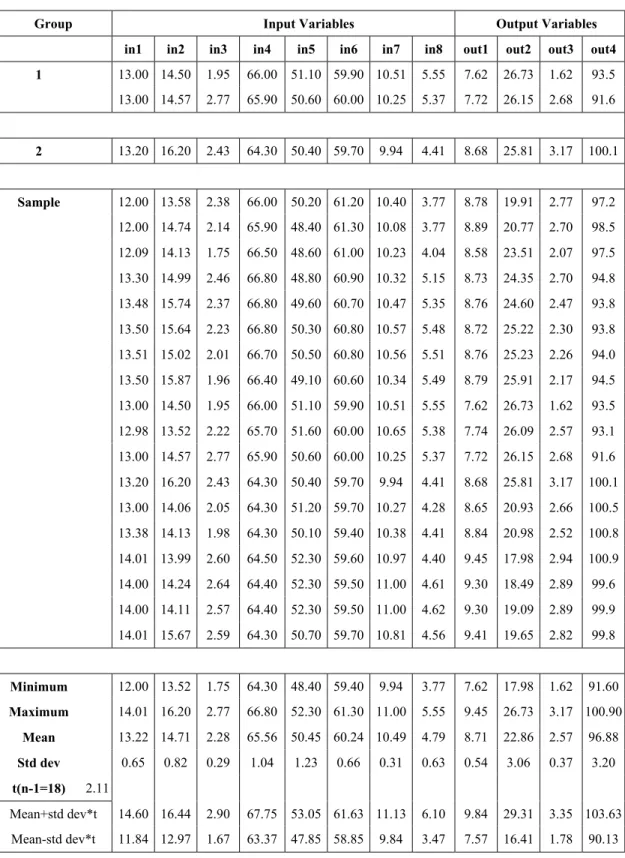
when there are only two data sets for comparison with some different information, it is not possible to determine which one is correct. In these cases, the domains of the variables are extended, compared with the previous group. Although these new groups are less accurate, it is usually possible to identify abnormal points. For this step, the hypothesis test for means, which involves a confidence interval estimate and a hypothesis test was employed with a confidence level of 95% (Himmelblau, 1970).
Table 2 shows the application of this methodology in analysis of plant data. The values in bold in groups 1 and 2 were not well adjusted during neural network training and it was not possible to identify groups of similar data sets for the cluster analysis; thus a hypothesis test for means analysis was performed. It was observed that the value 25.81 is inside the confidence interval and the null hypothesis is accepted and this data must not be eliminated. On the other hand, the value 1.62 is outside the confidence interval and the null hypothesis is rejected and this data set must be eliminated.
Figure1: Data analysis methodology
Table 1: Cluster analysis - examples
Input Variables Output Variables
in1 in2 in3 in4 in5 in6 in7 in8 out1 out2 out3 out4
12.79 15.34 1.86 63.80 39.30 59.90 8.89 4.37 8.35 25.24 2.50 97.4 12.80 15.40 1.88 63.80 39.20 59.90 8.87 4.35 8.35 27.21 2.63 97.3 12.80 15.25 1.79 63.80 39.20 59.90 8.85 4.38 8.35 26.88 2.53 97.4 12.75 15.07 1.71 63.80 39.10 59.80 8.79 4.36 8.35 27.21 2.49 97.3
Table 2: Hypothesis test for means
Group Input Variables Output Variables in1 in2 in3 in4 in5 in6 in7 in8 out1 out2 out3 out4
1 13.00 14.50 1.95 66.00 51.10 59.90 10.51 5.55 7.62 26.73 1.62 93.5 13.00 14.57 2.77 65.90 50.60 60.00 10.25 5.37 7.72 26.15 2.68 91.6
2 13.20 16.20 2.43 64.30 50.40 59.70 9.94 4.41 8.68 25.81 3.17 100.1
Sample 12.00 13.58 2.38 66.00 50.20 61.20 10.40 3.77 8.78 19.91 2.77 97.2 12.00 14.74 2.14 65.90 48.40 61.30 10.08 3.77 8.89 20.77 2.70 98.5 12.09 14.13 1.75 66.50 48.60 61.00 10.23 4.04 8.58 23.51 2.07 97.5 13.30 14.99 2.46 66.80 48.80 60.90 10.32 5.15 8.73 24.35 2.70 94.8 13.48 15.74 2.37 66.80 49.60 60.70 10.47 5.35 8.76 24.60 2.47 93.8 13.50 15.64 2.23 66.80 50.30 60.80 10.57 5.48 8.72 25.22 2.30 93.8 13.51 15.02 2.01 66.70 50.50 60.80 10.56 5.51 8.76 25.23 2.26 94.0 13.50 15.87 1.96 66.40 49.10 60.60 10.34 5.49 8.79 25.91 2.17 94.5 13.00 14.50 1.95 66.00 51.10 59.90 10.51 5.55 7.62 26.73 1.62 93.5 12.98 13.52 2.22 65.70 51.60 60.00 10.65 5.38 7.74 26.09 2.57 93.1 13.00 14.57 2.77 65.90 50.60 60.00 10.25 5.37 7.72 26.15 2.68 91.6 13.20 16.20 2.43 64.30 50.40 59.70 9.94 4.41 8.68 25.81 3.17 100.1 13.00 14.06 2.05 64.30 51.20 59.70 10.27 4.28 8.65 20.93 2.66 100.5 13.38 14.13 1.98 64.30 50.10 59.40 10.38 4.41 8.84 20.98 2.52 100.8 14.01 13.99 2.60 64.50 52.30 59.60 10.97 4.40 9.45 17.98 2.94 100.9 14.00 14.24 2.64 64.40 52.30 59.50 11.00 4.61 9.30 18.49 2.89 99.6 14.00 14.11 2.57 64.40 52.30 59.50 11.00 4.62 9.30 19.09 2.89 99.9 14.01 15.67 2.59 64.30 50.70 59.70 10.81 4.56 9.41 19.65 2.82 99.8
Minimum 12.00 13.52 1.75 64.30 48.40 59.40 9.94 3.77 7.62 17.98 1.62 91.60 Maximum 14.01 16.20 2.77 66.80 52.30 61.30 11.00 5.55 9.45 26.73 3.17 100.90
Mean 13.22 14.71 2.28 65.56 50.45 60.24 10.49 4.79 8.71 22.86 2.57 96.88 Std dev 0.65 0.82 0.29 1.04 1.23 0.66 0.31 0.63 0.54 3.06 0.37 3.20 t(n-1=18) 2.11
RESULTS AND DISCUSSION
A simple measure to assess the quality of the fit of the chosen neural network to the experimental data is usually a comparison of the values calculated by the neural network with the original experimental data. The scatter of data points around the ideal 45o line can be used to judge the fit of the neural network to the experimental data. The idea to use neural networks for the purpose of outlier detection is based on this kind of diagram (Bülau et al., 1999). Hence, it must only be shown that the outliers of the experimental data correspond to the outliers from this curve. Thus, the
neural network was first of all trained for the entire data set and afterwards for the filtered data set. The outliers detected after the first training run were analyzed by application of the statistics described previously. This procedure was repeated several times until the scattered data no longer showed abnormal points. Since the training of the network with the filtered data leads to results for calculated data, which are different from those for the original data set, the input database changes due to the filtration procedure. Table 3 shows the number of eliminated points in each run and Figures 2a-c show the results of this method for the first, second and final runs, respectively.
Table 3: Points eliminated in each run
Run Number of points eliminated
1 49
2 28
3 19
4 7
5 12
6
(b)
(c)
CONCLUSIONS
Application of a neural network is a very attractive tool for detecting outliers. It is simple, more cost effective and more easily used, particularly by plant engineers, and the results presented demonstrate that neural networks have considerable potential in the field of data analysis, mainly because they require much less knowledge of the underlying physicochemical process. However, the final decision to eliminate the suspect data is made by applying a cluster analysis to this approach to detect outliers.
ACKNOWLEDGMENTS
The authors gratefully acknowledge FAPESP for its financial support and COPENE Petroquímica do Nordeste for providing the industrial data used in this work.
REFERENCES
Bhat, N. and McAvoy, T.J. (1990). Use of Neural Nets for Dynamic Modeling and Control of Chemical Process Systems. Comput. Chem. Eng., 14 (4/5), 575.
Bülau, H.C., Ulrich, J., Guardani, R. and Nascimento, C.A.O. (1999). Application of Neural Networks to Data from a Melt Crystalization Process for the Detection of Outliers. In Proceedings of AIDA, International Seminar on Advances in Data Analysis – Washington, DC.
Giudici, R., Nascimento, C.A.O., Tresmondi, A., Domingues, A. and Pellicciotta, R. (1999). Mathematical Modeling of an Industrial Process of Nylon-6,6 Polymerization in a Two-Phase Flow Tubular Reactor. Chem. Eng. Sci., 54, 3242. Himmelbalu, D.M. (1970). Process Analysis by
Statistical Methods. John Wiley & Sons, Inc. Hoskins, J.C. and Himmelblau, D.M. (1988).
Artificial Neural Network Models for Knowledge Representation in Chemical Engineering. Comput. Chem. Eng., 12 (9/10), 881.
Nascimento, C.A.O. and Giudici, R. (1998). Neural Network Based Approach for Optimization Applied to an Industrial Nylon-6,6 Polymerization Process. Comput. Chem. Eng., 22, S595.
Nascimento, C.A.O., Giudici, R. and Guardani, R. (2000). Neural Network Based Approach for Optimization of Industrial Chemical Processes. Comput. Chem. Eng., 24, 2303.