ISSN 0104-6632 Printed in Brazil
www.abeq.org.br/bjche
Vol. 33, No. 03, pp. 607 - 616, July - September, 2016 dx.doi.org/10.1590/0104-6632.20160333s20150050
Brazilian Journal
of Chemical
Engineering
LINEAR STABILITY ANALYSIS AND CFD
SIMULATION OF DOUBLE-LAYER
RAYLEIGH-BÉNARD CONVECTION
É. Fontana
1,2*, E. Mancusi
1,3, A. A. Ulson De Souza
1and S. M. A. Guelli U. Souza
1 1Universidade Federal de Santa Catarina, Departamento de EngenhariaQuímica e de Alimentos, 88040-970, Florianópolis - SC, Brazil. Phone/Fax: (55) (48) 3721 3375
*E-mail: [email protected]
E-mail: [email protected]; [email protected]
2Universidade Federal de Santa Catarina, Campus Blumenau, 89065-300, Blumenau - SC, Brazil. 3Università del Sannio, Facoltà di Ingegneria, 82100 Benevento, Italy.
E-mail: [email protected]
(Submitted: January 26, 2015 ; Revised: June 1, 2015 ; Accepted: September 12, 2015)
Abstract - Natural convection in superimposed layers of fluids heated from below is commonly observed in many industrial and natural situations, such as crystal growth, co-extrusion processes and atmospheric flow. The stability analysis of this system reveals a complex dynamic behavior, including the potential multiplicity of stationary states and occurrence of periodic regimes. In this study, a linear stability analysis (LSA) was performed to determine the onset of natural convection as a function of imposed boundary conditions, geometrical configuration and specific perturbations. To investigate the effects of the non-linear terms neglected in LSA, a direct simulation of the full nonlinear problem was performed using computational fluid dynamics (CFD) techniques. The numerical simulation results show an excellent agreement with the LSA results near the onset of convection and an increase in the deviation as the Rayleigh number increases above the critical value.
Keywords: Hydrodynamic Stability; Natural Convection; Multiphase Flow.
INTRODUCTION
Single layer Rayleigh-Bénard (RB) convection is one of the most widely studied systems in the field of transport phenomena, mainly due to the large number of applications and the relative simplicity of the gov-erning equations. This system represents a natural convection condition occurring in a horizontal layer of fluid where energy is added from below and removed from above, giving rise to cellular structures called Bénard cells (or convective cells) when the buoyancy forces are sufficiently stronger than the viscous forces. Even though it has been investigated for more than a century, the RB problem has been the subject of a large number of studies in recent years,
involving, in particular, modifications of the classical RB system. For example, the problem of natural and mixed convection in enclosures is very important in the study of the cooling of electronic devices and ther-mal comfort (Fontana et al., 2015; An et al., 2013; Mariani and Coelho, 2007).
basically by conduction. However, when this critical value is exceeded the system becomes unstable and evolves to a different equilibrium state where natural convection is the main heat transfer mechanism. In bifurcation theory terminology, under this condition a bifurcation occurs and the critical point corresponds to a bifurcation point.
Different methods can be applied to investigate the RB system stability, and linear stability analysis (LSA) one of the most commonly used. Although the basics of LSA were first described more than a century ago, this method is still a very useful and powerful tool which is widely used in the study of fluid dynamics systems (e.g., Sahu and Matar, 2010; Fontana et al., 2015a; Sahu and Govindarajan, 2012; Travnikov et al., 2015). Due to a rapid increase in the data pro-cessing capacity, LSA studies are reaching a new frontier where the stability of more complex systems can be analyzed in a short amount of time. However, there are drawbacks associated with LSA, especially due to the non-linear terms neglected in this method of analysis. The main objective of this study was to compare the LSA results with CFD simulations car-ried out using state-of-the-art software packages where the full non-linear form of the governing equa-tions is considered.
Through linear stability analysis it is possible to define the critical Rayleigh values (Rac) as well as the wavenumber associated with the perturbation that first makes the RB system unstable (c). As de-scribed by Pellew and Southwell (1940), for unbound two-dimensional systems with Newtonian fluids, the critical parameters are governed only by the boundary conditions applied to the velocity vectors at both horizontal boundaries, which can be treated as rigid walls or free surfaces. The values obtained consider-ing the possible combinations, summarized in Table 1, show that the presence of a rigid wall significantly in-creases the critical parameters, stabilizing the system. In the CFD simulations, the change in the steady-state condition can be observed by a sudden increase in the Nusselt number as the Rayleigh number is increased. When conduction is the only heat transfer mechanism, the Nusselt number is constant, while the presence of convective motion causes an increase in the Nusselt number.
The presence of a second fluid layer significantly increases the system complexity and can affect the stability in many ways, for example, through competi-tion between convective modes in each layer, control of the flow in one layer over the flow in the other, interface deformation and unstable convective modes controlled by interfacial tension gradients. Several
important aspects of the stability of multi-layer fluid systems have been known for decades, for example, those related to the Kelvin-Helmholtz and Rayleigh-Taylor instabilities (Chandrasekhar, 1961). Neverthe-less, due to the complex dynamic behavior and the large number of governing parameters, stability analy-sis of the flow involving superimposed layers of fluids has been studied by several authors in recent years (Mishra et al., 2012; Kushnir et al., 2014; Sahu and Govindarajan, 2011; Redapangu et al., 2012) and is still an ongoing topic in the field of fluid dynamics.
Table 1: Critical parameters for single layer Ray-leigh-Bénard convection (Pellew and Southwell, 1940).
Boundary condition Rac c
Rigid – rigid 1707.8 3.117 Rigid – free 1100.7 2.682 Free – free 657.5 2.221
Besides the theoretical importance in the field of stability analysis, the study of the stability of natural convection in multi-layer systems plays an important role in several practical applications, as noted by Anderek et al. (1998). Systems where stratification occurs due to differences in density or thermal proper-ties are fairly common in the analysis of geophysical systems, atmospheric flow, astrophysics and indus-trial processes. The study of these systems was origi-nally motivated by the hypothesis that the Earth’s mantle is stratified as a result of a seismic discontinu-ity observed at a depth of approximately 660 km (Ogawa, 2008). In recent decades the study of double-layer natural convection was extended to several tech-nological applications of significant interest in the chemical engineering field, such as liquid encapsu-lated techniques for crystal growth (Li et al., 2009), the processing of glass and dispersion materials (Prakash, 1997), micro-channel chemical reactors (Fudym et al., 2007) and the processing of electronic materials under micro-gravity conditions (Gupta et al., 2007).
Linear Stability Analysis and CFD Simulation of Double-Layer Rayleigh-Bénard Convection 609
stability analysis due to its relative simplicity and flexibility. However, this method has intrinsic limita-tions derived from the fact that high-order terms are neglected in the linearization process. In this study, direct simulation of the full non-linear set of govern-ing equations usgovern-ing modern computational fluid dynamics (CFD)-based techniques was performed and the results compared with those obtained through linear stability analysis (LSA) in order to evaluate the comparative performance of each method.
MATHEMATICAL MODEL
A scheme of the geometrical configuration con-sidered is shown in Figure 1. The system consists of two layers of immiscible fluids confined between horizontal rigid walls. The system is assumed to be unbound in the z and x directions; however, perturba-tions in these direcperturba-tions are also included in the model. The thickness of the lower layer, d1 , is used as the length scale with the bottom wall placed at the dimen-sionless position y 1 and the upper wall placed at
2/ 1 0
y d d d , where d2 represents the height of the upper layer. The temperatures of these two walls are considered to be constant and the analysis was limited to the case TH TC where TH is the tempera-ture of the bottom wall and TC the temperature of the top wall. The non-deformed interface is positioned at
0
y and the interface deformation is evaluated
using the function ( , , )x z t .
Figure 1: Physical domain.
Each layer has its own set of governing equations, these equations being linked by the boundary condi-tions at the interface. It is assumed that the flow in both layers is incompressible, the fluids have Newto-nian behavior and the Boussinesq approximation is valid for the entire range of conditions evaluated. Under these conditions the governing equations are the standard Navier-Stokes and energy and mass conservation equations. No-slip and no-penetration boundary conditions are applied to the velocity vector at the solid walls (y 1 and yd0 ), while fixed
temperatures are defined at the same locations. At the interface (y), conditions of normal and tangential velocity continuity, as well as the shear and normal stress balance, are used to determine the velocity field, while for the energy conservation equation conditions of temperature and heat flux continuity are assumed.
In order to characterize the stability properties of a given base state through linear stability analysis, the variables in the set of governing equations are ex-pressed as the sum of the base state and an infinitesi-mal perturbation, and thus the dynamic behavior of these perturbations can be used to define the state stability: if the perturbations decrease over time and eventually disappear the system will be stable, other-wise it will be unstable. In LSA only infinitesimal perturbations are considered and thus all of the high-order terms can be neglected. Moreover, non-dimen-sional variables will be introduced by using d1 as the length scale, 1/d1 as the scale for the perturbation velocity, 1 1 1/d12 for the pressure and 1 1d as the scale for the temperature, where 1 , 1 and 1 are, respectively, the thermal diffusivity, density and kine-matic viscosity of the lower layer and 1 is the static temperature gradient between the non-deformed inter-face and the bottom wall.
The base state represents a solution for the set of governing equations and the related boundary condi-tions. In this case, the base state is associated with the horizontal velocity (UB,1,UB,2) and temperature
,1, ,2)
B B
(T T in the lower (1) and upper (2) layers. To
determine the onset of natural convection in a double-layer RB convection system, the base state corre-sponds to the stationary fluid (UB,1UB,20) with a linear temperature profile associated with heat transfer only by conduction, given by:
,1 1( 1)
B H
T T ψ y (1)
,2 2( 0)
B C
T T ψ y d (2)
where 2 is the static temperature gradient between the top wall and the non-deformed interface.
( ) ( , , , ) ( ) i x z t
s x y z t s y e (3)
where s y( ) is the eigenfunction associated with the original variable, and are wavenumbers in the x and z directions, respectively, and rii is the wave velocity, where r is the phase velocity and i the temporal growth rate of the perturbation. A condi-tion where i0 represents a damped perturbation and a stable system, while in cases where i0 the perturbation will grow and the base state will be un-stable. The condition i 0 is called neutral stability and represents a bifurcation point where the change in the steady-state solution occurs. The main objective of LSA is to obtain the values for the parameters where this bifurcation point occurs. In this study, we limit our analysis to temporal instabilities. Thus, the wavenumbers and are real values, which are used as parameters to find the critical Rayleigh number. After some manipulation, the pressure can be elimi-nated and the equations governing the system stability in the lower layer can be expressed as (see Fontana (2014) and Fontana et al. (2015a) for details):
2 4 2
2
1 1 1
1
2 4 2
4 2 1 1 2 Pr
i d d d
k k
dy dy dy
k k Ra
(4)
2 2 1
1 1 2 1
i d k dy
(5)
where 1 and 1 represent the perturbation of the ver-tical velocity and temperature, respectively, k2 is de-fined as k222 and the Prandtl and Rayleigh numbers are given by:
4
1 1 1 1
1 1 1
Pr
Ra
g d
(6)where 1 is the coefficient of thermal expansivity of the lower layer and g is the gravitational acceleration. The equations for the upper layer (denoted by the subscript 2) can be expressed as:
2 2 2 2 2 4 2
2 4 2
2 2
0 4 2 2 0 2
Pr 2 i d k dy d d
k k k Ra
dy dy (7) 2 2 2
2 0 2 0 2 2
d i k dy
(8)
where the subscript 0 denotes the relation between the parameter evaluated at the upper and at the lower layer.
As demonstrated by Hesla et al. (1986), when the fluids are considered incompressible, homogeneous, immiscible and with constant interfacial tension, Squire’s theorem is valid and only two-dimensional perturbations need to be considered to determine the lowest Rayleigh value where the system becomes unstable. Therefore, the condition 0 will be used to determine the system stability, which implies that
2 2
k .
The no-penetration condition applied at the solid walls (y 1 and yd0) can be expressed as:
1 20
(9)
while the no-slip conditions gives:
1 2 0
d d
dy dy
(10)
At the non-deformed interface (y0), the conti-nuity of normal and tangential velocities, respectively, is given by:
1 2
(11)
1 2 0
d d
dy dy
(12)
The continuity of shear stress at the interface (neglecting the thermocapillary effect) results in:
2 2
2 1 2 2 2
1 2 2 2 0
d d
k m k k
dy dy
(13)
where m is the relation between the dynamic viscosity in the upper and lower layers and 0 is the dimen-sionless interface deformation expressed in terms of normal modes. Using the kinematic condition, 0 can be expressed as:
1 0 (0) i
(14)
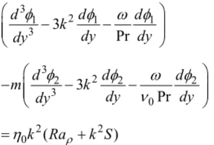
Linear Stability Analysis and CFD Simulation of Double-Layer Rayleigh-Bénard Convection 611 (7) is the balance of normal stress at the interface,
given by:
3 2
1 1 1
3
3
2
2 2 2
3 0 2 2 0 3 Pr 3 Pr ( )
d d d
k
dy dy
dy
d d d
m k
dy dy
dy
k Ra k S
(15)
where the interfacial tension-based Schmidt ( )S number and a Rayleigh number based on the density difference between the upper and lower layers (Ra)
are defined as:
2
1 1 1
1 1 1 1 1 1
3
1 2
1 1 1
1
d d d
Ma S dT gd Ra (16)
where is the interfacial tension and T is the tem-perature.
The conditions of fixed temperature at the solid walls (y 1 and yd0) are expressed as:
1 20
(17)
while the conditions of continuity of temperature and heat flux at the interface give, respectively:
1 2 0(1 0)
(18)
1 2 0 d d k dy dy (19)
To solve the generalized eigenvalue problem ob-tained, a pseudo-spectral method using Chebyshev polynomials was applied (see Canuto et al. (2006) for further details). For example, the perturbation in the temperature of the bottom layer, 1, is expressed as:
1 1 0 ( )
k N k k k T y (20)
where Tk is the Chebyshev polynomial of order k and
1
k
is the coefficient associated with Tk. To validate
the resolution methodology, stability curves obtained with the proposed method were compared with results reported by Cardin et al. (1991), as seen in Figure 2. An excellent agreement between the results can be observed, even considering the existence of a periodic state. The two branches of solution observed in this figure correspond to the two most unstable modes and the merging of these branches through a Hopf bifurca-tion gives rise to the periodic state.
Figure 2: Comparison between the stability curves presented by Cardin et al. (1991) (lines) and those obtained with the proposed methodology (points). These results correpond to the case d00.76, k00.54,
00.77,
01.27,00.67,01.92, Pr8400, 0
S and Ra10.
Direct simulation analysis based on CFD tech-niques was performed using the ANSYS Fluent 14.0 software, where the set of governing equations is dis-cretized through a multigrid finite volume approach. The ANSYS-CFD package is widely used to solve natural convection problems with high accuracy (see Fontana et al. (2011, 2013a) and Ghalambaz et al. (2014), for example). The hypothesis applied, the governing equations and the boundary conditions applied at the solid walls used in the CFD simulation are the same as those previously described for the LSA. To evaluate the interface deformation, the vol-ume of fluid (VOF) method was used. This method computes the interface position based on the velocity and pressure fields and therefore it is not necessary to specify the interface shape or even the boundary conditions at the interface, since these are directly obtained by the method. Further details regarding the VOF method can be found in Fontana et al. (2013) and Mancusi et al. (2014). A grid convergence test was performed and we found that a mesh with around 105 elements is sufficient to keep the solution stable
non-uniform elements distribution was used, with a greater concentration of elements close to the inter-face and the solid walls, where more intense gradients in the field variables are expected. To define the time-steps used, the Courant number was set to one. This condition resulted in time-steps of the order of seconds, depending on the intensity of the convective motion.
RESULTS
The physical properties were chosen so that the Rayleigh numbers for the two layers were the same when d01.0 (01 , 01 , 01 , 01 and
01
k ). Unless otherwise stated, these values were used to obtain all results discussed below. Moreover, the conditions Pr1 and Ra 105 are considered. This Ra value corresponds to a common value found
in the laboratory experiments. As noted by Go-vindarajan and Sahu (2014), one of the most im-portant parameters in double-layer convection is the viscosity difference in each layer. Thus, several au-thors have investigated the effect of a viscosity difference in double-layer Rayleigh-Bénard convec-tion (see Rasenat et al. (1988) and Cardin et al. (1991), for example). In this paper, we also assume that m1 in order to investigate the effect of the other parameters, in particular the relation between the thickness of each layer.
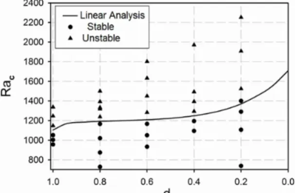
Figure 3 shows the stability limit curve obtained through LSA, where the critical Rayleigh number is presented as a function of the depth of the upper layer
0
(d ). The points obtained by CFD simulation for several d0 values are also reported in Figure 3. These points are classified as stable or unstable, depending on the presence or not of convective motion.
As can be seen in Figure 3, the limits defined by
the linear stability analysis are in excellent agreement with the results of the CFD simulations, with only one stable point appearing in the unstable region. How-ever, around the critical value, the onset of convection is not easily defined in the CFD simulations, since a theoretically infinite time would be necessary for a stationary convective state to be developed. It should be noted that the Rac values obtained in the cases
00.0
d and d01.0 correspond exactly to the values for the critical Rayleigh number for single layer RB convection when, respectively, rigid-rigid walls and rigid wall-free surface conditions are considered (see Table 1). This indicates complete consistency between the double and single-layer models.
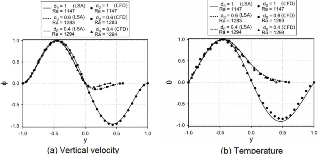
Besides the onset of convection, the LSA allows the spatial distribution of the velocity and temperature fields to be obtained through eigenfunctions. A com-parison between these eigenfunctions and the actual velocity and temperature profiles (deviation from the base state) obtained from the CFD simulations is shown in Figure 4 for d00.8 and Ra close to the critical value.
The profiles obtained from the LSA and the CFD simulation of the full nonlinear problem show ex-cellent agreement, in particular in relation to the ve-locity profiles. Despite a small deviation in the mag-nitude in comparison with the CFD results, the LSA eigenfunctions of the temperature deviation show the same tendency. A small change in the Rayleigh number does not affect significantly the profiles in any of the cases. A consistency in the eigenfunctions can also be observed for different d0 values, as re-ported in Figure 5. The Rayleigh values adopted for each case correspond to the unstable point closest to the critical point in Figure 3. These results show that, despite all of the simplifications and approximations made in the linearization process, LSA is able to describe very well the system behavior near the critical point.
Linear Stability Analysis and CFD Simulation of Double-Layer Rayleigh-Bénard Convection 613
Figure 4: Comparison between eigenfunctions obtained through LSA and velocity and temperature profiles obtained with CFD simulations for d00.8.
Figure 5: Comparison between eigenfunctions obtained through LSA and velocity and temperature profiles obtained with CFD simulations d0=1.0, 0.6 and 0.4.
One of the most restrictive hypothesis of the LSA using normal modes is that the interface deformation is not strong enough for the high-order terms to be neglected. In other words, this condition can be ex-pressed as d1. On the other hand, the main ad-vantage of using the VOF method to investigate double-layer convection is that it is possible to track the interface position at each point as a function of the velocity and temperature fields. The interface defor-mation is controlled by the normal stress balance, in particular by the value of Ra. If this value is not
high enough to keep the interface stable, surface waves will emerge and eventually the system will
shift to an unstable state. The condition Ra 0 will
not be considered since it represents, by definition, a Rayleigh-Taylor instability condition.
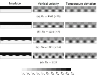
The vertical velocity and temperature deviation profiles, obtained through CFD simulations, are shown in Figure 6 for Ra 103 and d01.0, together with the interface position for several values of Ra Rac.
To facilitate the visualization of the results, allowing the use of a single legend, the values for Ra1425 were multiplied by a scale, as indicated in the figure for each case.
approximately 1163 and therefore the results shown in Figure 6(a) are very close to the critical value. In this case, the interface deformation can be neglected and the velocity and temperature profiles are similar to those obtained at higher Ravalues. For Ra1234
(Figure 6(b)), a small deformation in the interface po-sition can be observed; however, the condition
1
d
still holds true and the velocity and tempera-ture profiles are very similar to Ra1163.
Figure 6: Influence of interface deformation on ve-locity and temperature fields for Ra 103.
Even though the interface deformation is negligi-ble when ܴܽ is close to the critical value, as the Ray-leigh number increases it becomes stronger, as seen in Figure 6. For Ra1371 (Figure 6(c)) the velocity profiles are significantly different and the convective cells become distorted. The interface acquires a wavy shape, with the maximum points (crest) appearing in the region where the fluid ascends, and the vertical velocity in the lower layer is positive near the inter-face and the minimum points appear in the descending region. For Ra1425 the deformations further in-crease and the deviation from the linearized model is more significant.
CONCLUSIONS
In this paper a comparison between linear stability analysis using normal modes and numerical simula-tion (with CFD techniques) of double-layer Rayleigh-Bénard convection has been presented. LSA tech-niques allow the determination of the critical value at which the convection starts; however, the lineariza-tion process neglects high-order terms and this can lead to deviations from the actual system behavior.
The CFD simulations, on the other hand, solve the full non-linear system of governing equations, but they are much more computationally expensive. The results show that the performance of LSA is excellent near the critical point and thus it can be used to define the critical values. Moreover, at this limit the velocity and temperature profiles obtained with LSA accurately describe the system behavior. However, as the inten-sity of the convective motion increases, the deviations from the linearized model increase and the velocity and temperature profiles given by the LSA are no longer consistent. In particular, a higher velocity at the interface leads to the development of interfacial waves, causing a strong deformation in the tempera-ture and velocity fields.
ACKNOWLEDGMENTS
The authors would like to thank the CNPq (Con-selho Nacional de Desenvolvimento Científico e Tecnológico – Brazil) for financial support through the process 143152/2011-4.
NOMENCLATURE
d Fluid layer thickness (m)
g Acceleration of gravity (m/s2
)
Pr Prandtl number (–)
Ra Rayleigh number (–)
Ra Density-based Rayleigh number (–)
S Interfacial tension-based Schmidt number
(–)
T Temperature (K)
C
T Temperature of the upper wall (cold) (K)
H
T Temperature of the bottom wall (hot) (K)
k
T Chebyshev Polynomial of order k (–)
U Horizontal velocity (m/s)
x Dimensionless horizontal direction (–)
y Dimensionless vertical direction (–)
z Dimensionless transversal direction (–)
Greek Letters
Perturbation wavenumber in the x direction
(–)
Perturbation wavenumber in the z direction
(–)
i
Thermal expansion coefficient of the i-fluid (1/K)
Linear Stability Analysis and CFD Simulation of Double-Layer Rayleigh-Bénard Convection 615
Interface deformation (m)
Perturbation of the temperature (–)
Thermal diffusivity (m2/s)
Kinematic viscosity (m2/s)
Fluid density (kg/m3
)
Perturbation of the vertical velocity (–)
Static temperature gradient (K)
Wave velocity/eigenvalue (–)
Subscripts
B Base state
c Critical value
0 Ratio between upper and lower layer
1 Lower layer
2 Upper layer
REFERENCES
An, C., Vieira, C. B., Su, J., Integral transform solu-tion of natural convecsolu-tion in a square cavity with volumetric heat generation. Braz. J. Chem. Eng., 30(4), p. 883-896 (2013).
Anderek, C. D., Colovas, P. W., Degen, M. M., Re-nardy, Y. Y., Instabilities in two layer Rayleigh-Bénard convection: Overview and outlook. Int. J. Eng. Sci., 36, p. 1451-1470 (1998).
Canuto, C., Hussaini, M. Y., Quarteroni, A., Zang, T. A., Spectral Methods: Fundamentals in Single Do-mains. [S.l.], Springer (2006).
Cardin, P., Nataf, H. C., Dewost, P., Thermal coupling in layered convection: evidence for an interface viscosity control for mechanical experiments and marginal stability analysis. J. Physics II, 1, p. 599-622 (1991).
Chandrasekhar, S., Hydrodynamic and Hydromagnetic Stability. [S.l.], Clarendon Press (1961).
Fontana, É., Silva, A., Mariani, V. C., Natural convec-tion in a partially open square cavity with internal heat source: An analysis of the opening mass flow. Int. J. of Heat and Mass Transfer, 54, p. 1369-1386 (2011).
Fontana, É., Mancusi, E., Souza, A. A. U., Souza, S. M. A. G. U., Flow regimes for liquid water trans-port in a tapered flow channel of proton exchange membrane fuel cells (PEMFCs). J. Power Sources, 234, p. 260-271 (2013).
Fontana, É., Capeletto, C. A., Silva, A., Mariani, V. C., Three-dimensional analysis of natural convection in a partially-open cavity with internal heat source. Int. J. of Heat and Mass Transfer, 61, p. 525-542 (2013a).
Fontana, É., Análise de estabilidade da convecção de Rayleigh-Bénard-Poiseuille estratificada. PhD Thesis, Universidade Federal de Santa Catarina (2014). (In Portuguese).
Fontana, É., Capeletto, C. A., Silva, A., Mariani, V. C., Numerical analysis of mixed convection in par-tially open cavities heated from below. Int. J. of Heat and Mass Transfer, 81, p. 829-845 (2015). Fontana, É., Mancusi, E., Souza, A. A. U., Souza, S.
M. A. G. U., Stability analysis of stratified Rayleigh-Bénard-Poiseuille convection: Influence of the shear flow. Chem. Eng. Sci., 126, p. 67-79 (2015a). Fudym, O., Pradere, C., Batsale, J. C., An analytical two-temperature model for convection–diffusion in multilayered systems: Application to the ther-mal characterization of microchannel reactors. Chem. Eng. Sci., 62, p. 4054-4064 (2007).
Ghalambaz, M., Noghrehabadi, A., Ghanbarzadeh, A., Natural convection of nanofluids over a con-vectively heated vertical plate embedded in a po-rous medium. Braz. J. Chem. Eng., 31(2), p. 413-427 (2014).
Govindarajan, R., Sahu, K. C., Instabilities in viscos-ity- stratified flow. Annu. Rev. Fluid Mech., 46, p. 331-353 (2014).
Gupta, N. R., Hariri, H. H., Borhan, A., Thermocapil-lary convection in double-layer fluid structures within a two-dimensional open cavity. J. of Colloid and Interface Science, 315, p. 237-347 (2007). Hesla, T. I., Pranckh, F. R., PreziosI, L., Squire’s
theo-rem for two stratified fluids. Phys. of Fluids, 29, p. 2808-2811 (1986).
Kushnir, R., Segal, V., Ullmann, A., Brauner, B., In-clined two-layered stratified channel flows: Long wave stability analysis of multiple solution re-gions. Int. J. Multiphase Flow, 62, p. 17-29 (2014). Li, Y. R., Wang, S. C., Wu, S. Y., Peng, L., Asymptotic
solution of thermocapillary convection in thin annular two-layer system with upper free surface. Int. J. Heat and Mass Transfer, 52, p. 4769-4777 (2009).
Mancusi, E., Fontana, E., Ulson de Souza, A. A., Guelli U. Souza, S. M. A., Numerical study of two-phase flow patterns in the gas channel of PEM fuel cells with tapered flow field design. Int. J. Hydro-gen Energy, 39, p. 2261-2273 (2014).
Mariani, V. C., Coelho, L. S., Natural convection heat transfer in partially open enclosures containing an internal local heat source. Braz. J. Chem. Eng., 24(3), p. 375-388 (2007).
Ogawa, M., Mantle convection: A review. Fluid Dy-namics Research, 40, p. 379-398 (2008).
Pellew, A., Southwell, R. V., On maintained convec-tive motion in a fluid heated from below. Proc. of the Royal Society, 176(966), p. 312-342 (1940). Prakash, A., Yasuda, K., Otsubo, F., Kuwahara, K.,
Doi, T., Flow coupling mechanisms in two-layer Rayleigh-Bénard convection. Experiments in Fluids, 23, p. 252-261 (1997).
Rasenat, S., Busse, F. H., Rehberg, I., A theoretical and experimental study of double-layer con-vection. J. Fluid Mechanics, 199, p. 519-540 (1989).
Redapangu, P. R., Vanka, S. P., Sahu, K. C., Multi-phase lattice Boltzmann simulations of buoy-ancy-induced flow of two immiscible fluids with
different viscosities. Eur. J. Mech. B/Fluids, 34, p. 105-114 (2012).
Sahu, K. C., Govindarajan, R., Linear stability of double-diffusive two-fluid channel flow. J. Fluid Mech., 687, p. 529-539 (2011).
Sahu, K. C., Govindarajan, R., Spatio-temporal linear stability of double-diffusive two-fluid channel flow. Phys. Fluids, 24, 054103 (2012).
Sahu, K. C., Matar, O. K., Three-dimensional linear instability in pressure-driven two-layer channel flow of a Newtonian and a Herschel-Bulkley fluid. Physics of Fluids, 22, 112103 (2010).