Summertime elemental mercury exchange of temperate grasslands on an ecosystem-scale

www.atmos-chem-phys.net/8/7709/2008/ © Author(s) 2008. This work is distributed under the Creative Commons Attribution 3.0 License.

Chemistry

and Physics

Summertime elemental mercury exchange of temperate grasslands

on an ecosystem-scale

J. Fritsche1, G. Wohlfahrt2, C. Ammann3, M. Zeeman4, A. Hammerle2, D. Obrist5, and C. Alewell1 1_{Institute of Environmental Geosciences, University of Basel, Bernoullistrasse 30, 4056 Basel, Switzerland} 2_{Institute of Ecology, University of Innsbruck, Sternwartestrasse 15, 6020 Innsbruck, Austria}

3_{Agroscope Reckenholz-Taenikon Research Station ART, Air pollution/Climate group, Reckenholzstrasse 191,}

8046 Zurich, Switzerland

4_{Institute of Plant Science, ETH Zurich, Universitaetsstrasse 2, 8092 Zurich, Switzerland}

5_{Desert Research Institute, Division of Atmospheric Sciences, 2215 Raggio Parkway, Reno, NV 89512, USA}

Received: 1 October 2007 – Published in Atmos. Chem. Phys. Discuss.: 4 February 2008 Revised: 23 July 2008 – Accepted: 21 November 2008 – Published: 22 December 2008

Abstract. In order to estimate the air-surface mercury ex-change of grasslands in temperate climate regions, fluxes of gaseous elemental mercury (GEM) were measured at two sites in Switzerland and one in Austria during summer 2006. Two classic micrometeorological methods (aerodynamic and modified Bowen ratio) have been applied to estimate net GEM exchange rates and to determine the response of the GEM flux to changes in environmental conditions (e.g. heavy rain, summer ozone) on an ecosystem-scale. Both methods proved to be appropriate to estimate fluxes on time scales of a few hours and longer. Average dry deposition rates up to 4.3 ng m−2h−1 and mean deposition velocities up to 0.10 cm s−1were measured, which indicates that during the active vegetation period temperate grasslands are a small net sink for atmospheric mercury. With increasing ozone con-centrations depletion of GEM was observed, but could not be quantified from the flux signal. Night-time deposition fluxes of GEM were measured and seem to be the result of mercury co-deposition with condensing water. Effects of grass cuts could also be observed, but were of minor magnitude.

1 Introduction

The continued use of mercury in a wide range of products and processes and its release into the environment lead to de-position of mercury in ecosystems yet unspoiled. Its long at-mospheric lifetime of about 1 to 2 years (Lin and Pehkonen,

Correspondence to:J. Fritsche (johannes.fritsche@unibas.ch)

1999) enables elemental mercury (Hg0) to migrate to remote areas far away from its emission source, and once deposited to terrestrial or aquatic surfaces it is exposed to the formation of even more toxic methylmercury (IOMC, 2002). A suite of factors determines the ultimate fate of elemental mercury and its eventual immobilisation at the Earth’s surface. Depend-ing on atmospheric chemistry, meteorological conditions and physicochemical properties of the soils mercury may be cy-cled fairly rapidly between terrestrial surfaces and the atmo-sphere (Gustin and Lindberg, 2005). However, it remains un-clear whether deposited mercury is retained in background soils or whether terrestrial surfaces are even a net source of mercury (Pirrone and Mahaffey, 2005). Once deposited, mercury may be sequestered (e.g. adsorbed to soil organic matter and clay minerals), removed from the soil by leaching and erosion or re-emitted (Gustin and Lindberg, 2005). Mer-cury sequestered by terrestrial ecosystems might eventually be disconnected temporarily from the atmosphere-biosphere cycle, which would lead to a decrease in the pool of atmo-spheric mercury.

concentration was found to be the dominant factor associated with foliar mercury concentrations in different forb species (Fay and Gustin, 2007), and the successful application of dif-ferent grass species in biomonitoring studies (De Temmer-man et al., 2007) suggest that mercury uptake by plants is indeed of significance.

With innovations in sensitive measurement techniques in the last decade it is now possible to measure atmospheric mercury background concentrations currently ranging from 1.32 to 1.83 ng m−3(Valente et al., 2007). Such instruments also allow the estimation of air-surface exchange fluxes of gaseous elemental mercury (GEM) by applying micromete-orological methods. They are based on vertical concentration profiles and permit spatially averaged measurements without disturbing ambient conditions – an essential element of long-term studies.

During our previous work on GEM exchange of a mon-tane grassland in Switzerland we determined mean depo-sition rates of 5.6 ng m−2h−1 during the vegetation period (Fritsche et al., 2008). For that study GEM concentrations were measured for a whole year in order to describe the seasonal variation of the GEM exchange. In the current study that work is extended to another montane and one low-land grasslow-land site along the Alps with the aim to determine whether temperate grasslands in general are net sinks for at-mospheric mercury or whether GEM exchange is site spe-cific. Two classical micrometeorological methods are ap-plied to estimate the GEM fluxes: the aerodynamic method and the modified Bowen ratio (MBR) method. By perform-ing measurements durperform-ing the vegetation period, we test the potential and limitations of these two methods and also at-tempt to capture changes in the GEM flux caused by alter-ation of environmental conditions, e.g. grass cuts, heavy pre-cipitation, and elevated summer ozone concentrations.

2 Experimental

2.1 Site description

For our GEM flux measurements we selected three grass-land sites in Switzergrass-land and Austria with existing microm-eteorological towers. The first site, Fruebuel, is located on an undulating plateau 1000 m a.s.l. in central Switzerland. It is intensively used for cattle grazing and is bordered by forest, wetlands and other grasslands. The second location, Neustift, is an intensively managed, flat grassland in the Aus-trian Stubai Valley at an elevation of 970 m a.s.l. This previ-ously alluvial land lies between the Ruetz river and pastures and is primarily used for hay production. The third site is situated in Oensingen on the Swiss central plateau (Mittel-land) at 450 m a.s.l. between the Jura and the western Alps. It serves as an experimental farmland with extensive man-agement and neighbours agricultural land that borders on a motorway in the north-west.

All three sites are equipped with eddy covariance (EC) flux towers. The stations in Neustift and Oensingen are affiliated with the CarboEurope CO2 flux network and are operated

by the Institute of Ecology, University of Innsbruck, Austria and the Federal Research Station Agroscope ART, Switzer-land, respectively. At Fruebuel the EC flux tower is operated by the Institute of Plant Science, ETH Zurich to investigate greenhouse gas fluxes from agricultural land in the context of a changing climate.

Details about the meteorological and pedological condi-tions of all three sites are listed in Table 1. The predomi-nant wind direction at Fruebuel is SW to SSW, showing a distinct channelled flow as a result of the local, undulating, sub-alpine topography. The footprint of the EC flux measure-ments has been determined by using the footprint model of Kljun et al. (2004). For the EC sensor height of 2.55 m this resulted in a footprint coverage of>80% within a radius of 60 m. Within approximately 200 m of the predominant wind direction vegetation is homogenous and the calculated foot-print area covers the intensively managed part of the grass-land. Neustift on the other hand represents a site with the characteristic wind regime of an Alpine valley – the wind blowing into the valley from NE during the day and blowing out of the valley from SW during the night. Vegetation is uni-form for around 300 and 900 m in the directions of the day-and night-time winds, respectively, with the footprint max-imum lying within these boundaries for more than 90% of all cases. In Oensingen the fetch length is about 70 m along the dominant wind sectors (SW and NE) and 26 m in the per-pendicular axis. Using the footprint model of Kormann and Meixner (2001) the fraction of the field contributing to the measured EC CO2flux is>70% during most of the daytime,

whereas during night-times, this fraction is generally lower and highly variable due to very stable conditions. It has to be noted, that the fetch length is smaller than the heights of the GEM gradient measurements would require (see Sect. 2.4). However, for the benefit of higher vertical gradients on a well characterised grassland site this inadequacy was accepted.

The gleyic cambisols at Fruebuel and the stagnic cam-bisols at Oensingen are rather deep (>1 m), while the gleyic fluvisol in Neustift is very shallow (<30 cm). Total mer-cury concentrations at all sites are representative of un-contaminated background soils (see Table 1), although the Hgtotconcentration at Fruebuel lies at the threshold value of

100 ng g−1.

2.2 Micrometeorological methods

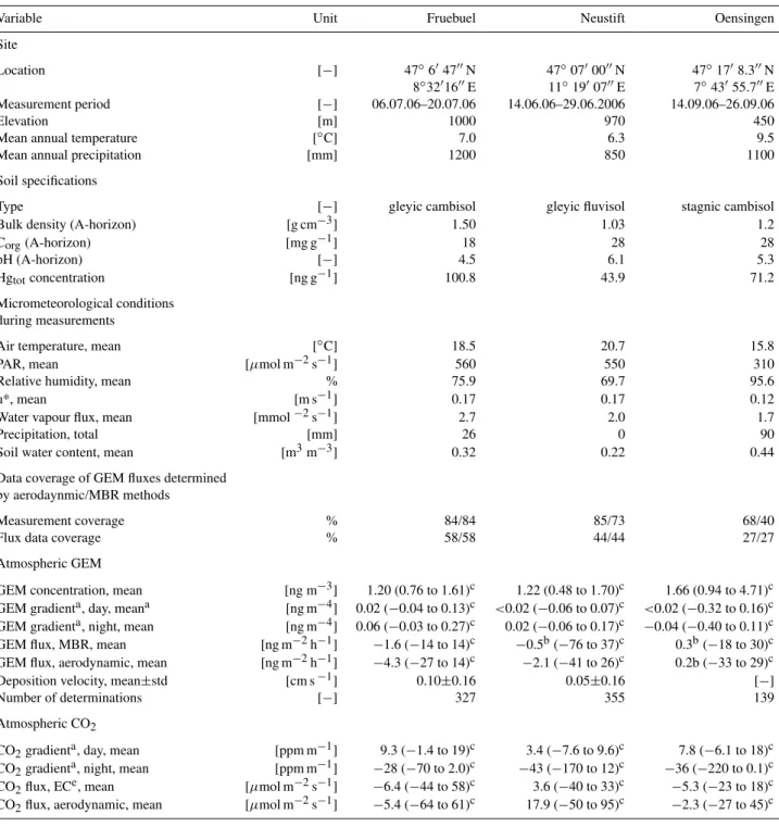
Table 1.Summary of site specifications, environmental conditions as well as atmospheric GEM and CO2data.

Variable Unit Fruebuel Neustift Oensingen

Site

Location [−] 47◦6′47′′N 47◦07′00′′N 47◦17′8.3′′N 8◦32′16′′E 11◦19′07′′E 7◦43′55.7′′E Measurement period [−] 06.07.06–20.07.06 14.06.06–29.06.2006 14.09.06–26.09.06

Elevation [m] 1000 970 450

Mean annual temperature [◦C] 7.0 6.3 9.5

Mean annual precipitation [mm] 1200 850 1100

Soil specifications

Type [−] gleyic cambisol gleyic fluvisol stagnic cambisol

Bulk density (A-horizon) [g cm−3] 1.50 1.03 1.2

Corg(A-horizon) [mg g−1] 18 28 28

pH (A-horizon) [−] 4.5 6.1 5.3

Hgtotconcentration [ng g−1] 100.8 43.9 71.2

Micrometeorological conditions during measurements

Air temperature, mean [◦C] 18.5 20.7 15.8

PAR, mean [µmol m−2s−1] 560 550 310

Relative humidity, mean % 75.9 69.7 95.6

u*, mean [m s−1] 0.17 0.17 0.12

Water vapour flux, mean [mmol−2s−1] 2.7 2.0 1.7

Precipitation, total [mm] 26 0 90

Soil water content, mean [m3m−3] 0.32 0.22 0.44

Data coverage of GEM fluxes determined by aerodaynmic/MBR methods

Measurement coverage % 84/84 85/73 68/40

Flux data coverage % 58/58 44/44 27/27

Atmospheric GEM

GEM concentration, mean [ng m−3] 1.20 (0.76 to 1.61)c 1.22 (0.48 to 1.70)c 1.66 (0.94 to 4.71)c GEM gradienta, day, meana [ng m−4] 0.02 (−0.04 to 0.13)c <0.02 (−0.06 to 0.07)c <0.02 (−0.32 to 0.16)c GEM gradienta, night, mean [ng m−4] 0.06 (−0.03 to 0.27)c 0.02 (−0.06 to 0.17)c −0.04 (−0.40 to 0.11)c GEM flux, MBR, mean [ng m−2h−1] −1.6 (−14 to 14)c −0.5b(−76 to 37)c 0.3b(−18 to 30)c GEM flux, aerodynamic, mean [ng m−2h−1] −4.3 (−27 to 14)c −2.1 (−41 to 26)c 0.2b (−33 to 29)c Deposition velocity, mean±std [cm s−1] 0.10±0.16 0.05±0.16 [−]

Number of determinations [−] 327 355 139

Atmospheric CO2

CO2gradienta, day, mean [ppm m−1] 9.3 (−1.4 to 19)c 3.4 (−7.6 to 9.6)c 7.8 (−6.1 to 18)c

CO2gradienta, night, mean [ppm m−1] −28 (−70 to 2.0)c −43 (−170 to 12)c −36 (−220 to 0.1)c

CO2flux, ECe, mean [µmol m−2s−1] −6.4 (−44 to 58)c 3.6 (−40 to 33)c −5.3 (−23 to 18)c

CO2flux, aerodynamic, mean [µmol m−2s−1] −5.4 (−64 to 61)c 17.9 (−50 to 95)c −2.3 (−27 to 45)c

a_{calculated as described in Sect. 2.5} b_{not significantly different from zero} c_range

d_{standard error}

e_{determined by eddy covariance}

therefore resorted to two more empirical methods. The first, the aerodynamic technique, is an application of Fick’s law of diffusion to the turbulent atmosphere (Baldocchi, 2006). Translated to an atmospheric trace gas the general relation-ship for the flux is

Fx= −Kx

∂cx

∂z (1)

whereFxis the vertical trace gas flux,Kxthe eddy

diffusiv-ity and∂cx/∂zthe concentration gradient of an arbitrary, non

reactive trace gasx(Dabberdt et al., 1993; Lenschow, 1995; Baldocchi, 2006). Corresponding equations have been for-mulated for the momentum flux (QM) as well as the fluxes

of sensible (QH) and latent heat (QE). It is assumed that the

sources and sinks of these scalars are equal and thus simi-larity between the eddy diffusivities (Kx=KH=KE) are

im-plied.

The eddy diffusivityKx is expressed by the aerodynamic

method as

Kx =

k×u∗×z

8h(z/L)

(2)

wherekdenotes the von Karman constant (0.4),u∗the fric-tion velocity, zthe measurement height, 8h(z/L) the

uni-versal temperature profile andLthe Monin-Obukhov length. Generally the eddy covariance technique is used to determine the friction velocity andLis calculated fromu∗, air temper-ature, air density and the sensible heat flux. By combination of Eq. (1) and Eq. (2) and subsequent integration we obtain

FGEM= −

k×u∗×(cGEMz2 −cGEMz1)

log(z2/z1)+ψz2−ψz1

(3)

whereψz1andψz2 are the integrated similarity functions for heat at the measured heights. A more detailed description of this method is given in Edwards et al. (2005).

The second method employed is the modified Bowen ratio method, which is a slightly more direct technique to estimate the GEM flux. This method uses directly measured fluxes of a surrogate scalar (i.e. sensible heat or a second trace gas) and the vertical gradient of this scalar. In our studies we mea-sured the fluxes of CO2with eddy covariance and its vertical

gradient concurrently with the GEM gradients. The GEM flux is then calculated as

FGEM=FCO2 ×

1cGEM

1cCO2

(4)

Further details and previous applications of this method are described by e.g. Meyers et al. (1996) and Lindberg and Meyers (2001).

2.3 Instrumentation

Air concentrations of GEM were measured in 5-min inter-vals with a dual cartridge mercury vapour analyser (Tekran 2536A, Tekran, Toronto, Canada). With this instrument mer-cury is preconcentrated by amalgamation and detected via cold vapour atomic fluorescence spectrometry; further details of its operation principals are described in e.g. Lindberg et al. (2000). The instrument was calibrated automatically every 24 h by means of an internal mercury permeation source. Ad-ditional, manual calibrations were performed prior to each measurement campaign by injecting mercury vapour with standard gas tight syringes from a mercury vapour genera-tion unit (Model 2505, Tekran, Toronto, Canada).

In order to compute GEM fluxes by the MBR method CO2

concentrations were measured with a closed path infrared gas analyser (LI-6262, LI-COR Inc., Lincoln, Nebraska, USA) at a frequency of 1 Hz. Before each campaign the gas analyser was calibrated with argon as zero gas and pressurised air with 451 ppm CO2as span gas. The zero-offset of argon relative

to a N2/O2gas mixture was 0.4 ppm.

Meteorological data (air temperature, net radiation, PAR, humidity, wind speed, wind direction) were recorded by the micrometeorological instrumentation of the towers at the study sites. Carbon dioxide and water vapour fluxes were de-termined by eddy covariance using three-dimensional sonic anemometers and open path infrared gas analysers (Solent R2 and R3, Gill Ltd., Lymington, UK, and LI-7500, LI-COR Inc., Lincoln, Nebraska, USA).

2.4 Measurement setup

The measurements were performed between June and September 2006 for two weeks at each site using the same in-struments. Vertical concentration gradients were determined by measuring GEM and CO2at 5 heights above ground (0.2,

0.3, 1.0, 1.6 and 1.7 m). The same setup was installed at all three sites, although the lowest sampling heights had to be adjusted to the local height of the vegetation (10–60 cm at Fruebuel and Neustift, and 10–20 cm at Oensingen). The sampling lines consisting of 1/4”-tubing were mounted to a mast in the vicinity of the micrometeorological towers and connected to a 5 port solenoid switching unit. Depending on space and the setup of the micrometeorological equip-ment at each site, the sampling lines were between 7 m and 15 m long. All lines had equal lengths and were cleaned be-fore each measurement series. Downstream of the switch unit, the Tekran instrument and the CO2analyser were

con-nected in series. Filter cartridges with 0.2µm Teflon® fil-ters were mounted to the inlets of the sampling lines to pre-vent contamination of the analytical system. Tubing and fit-tings made of Teflon® _{were used and cleaned with HNO}

3

mercury-free air generated by a zero air generator (Model 1100, Tekran, Toronto, Canada) before and after each mea-surement series. Additionally, by constricting the sampling lines temporarily it was tested if the setup had any leaks.

Air was sampled at a flow rate of 1.5 l min−1by the inter-nal pump of the Tekran instrument. To maintain continuous flushing of all sampling tubes an auxiliary pump with a flow rate of 6.0 l min−1was connected to the four lines that were currently not sampled. The sampled air was not dried, which required correction of the calculated fluxes for density effects (see below).

Air sampling was switched from a line at a lower height to one at an upper height every 10 min (i.e. the sequence with the heights mentioned above was 0.2–1.6–0.3–1.7–1.0 m). In this way a vertical concentration profile with five measure-ment points could be determined every 50 min. Higher fre-quencies were not feasible as the low ambient GEM concen-trations require pre-concentration by the gold cartridges of the Tekran intrument for accurate analysis.

2.5 Flux calculations

Upon completion of the measurement campaigns, GEM and CO2fluxes were computed with a self-programmed Matlab®

algorithm. Carbon dioxide fluxes were calculated to evaluate the quality of the GEM fluxes. By comparing the CO2fluxes

determined by the aerodynamic method with the CO2fluxes

obtained by eddy covariance we could assess the reliability of the aerodynamic method, i.e. matching CO2 fluxes lend

credibility to the calculated GEM fluxes (assuming the CO2

fluxes determined by EC to be accurate).

After correction of the GEM and CO2concentrations with

respect to the measured standards the atmospheric concentra-tion trend was subtracted from the data by interpolating the concentration measured at the top sampling line to the mea-surements of the other lines. This step was considered essen-tial as atmospheric concentrations changed during the course of a measurement cycle of 50 min (i.e. 20 min for one height pair) and overlaid the measured gradients. Next, GEM and CO2fluxes were calculated according to Eq. (3) and Eq. (4)

for four successive height pairs per measurement cycle. The raw fluxes were then obtained by computing the median of these four values, thus reducing uncertainty substantially.

As the sampled air was not dried the raw fluxes were cor-rected for density effects of water vapour according to Webb et al. (1980). A correction for sensible heat was not con-sidered necessary, because the sample air of all lines was brought to a common temperature before reaching the anal-ysers and because the Tekran instrument monitors the GEM concentration relative to the sampled air mass with a mass flow controller. Finally, the GEM and CO2flux data were

screened for outliers and values outside the range of the mean

±_{3 standard deviations of the whole period were rejected.}

3 Results

3.1 Data coverage

We performed our measurements at the three sites under fair weather conditions. However, due to power outages and showers during thunderstorms as well as instrument failures, not all variables required to calculate the GEM and CO2

fluxes could be measured continuously. As shown in Table 1 GEM fluxes could be computed for up to 85% of the mea-surement periods. In Neustift and Oensingen the data cover-age of the GEM fluxes calculated by the MBR method was considerably reduced due to failure of the eddy covariance systems.

As the resolution of gradient measurements is limited we determined the minimum resolvable gradient (MRG) in a similar way as described by Edwards et al. (2005). This was done once at Fruebuel by mounting all five sampling lines at 1 m above ground, measuring the GEM and CO2

con-centrations for three days and computing the concentration differences between the line pairs used for the flux calcu-lations. By defining the MRG as the mean of the concen-tration differences plus one standard deviation we obtained MRG’s of 0.02 ng m−3for GEM and 2.5 ppm for CO2. This

translates to minimum GEM fluxes determinable with the aerodynamic method of−_{2.8 to}−_{4.6 ng m}−2_h−1_{for typical}

daytime and−_{0.5 to}−_{1.9 ng m}−2_h−1_{for typical night-time}

turbulence regimes (for daytimeu∗=0.17 to 0.27 m s−1 and

z/L=−_{0.49 to}−_{0.16; for night-time}u∗=0.032 to 0.11 m s−1 andz/L=2.2 to 0.15, data from the Fruebuel site). As the MRG is system-specific, the values gained at Fruebuel were also applied to the measurements at Neustift and Oensingen. Excluding outliers and flux values with gradients below the MRG, the overall data coverage for the GEM fluxes at the three sites was between 27 and 58% (see Table 1 for details). However, exchange rates calculated with smaller gradients than the MRG were included in the results reported below, as average fluxes would otherwise be overestimated. 3.2 Meteorological conditions

Meteorological conditions at the three sites were mainly sunny and stationary most of the time (see Fig. 1 to 3 and Ta-ble 1). The measurement campaign in Oensingen was sched-uled for September 2006 when air temperature and irradi-ation were somewhat lower than at the other sites. How-ever, conditions in Oensingen were unstable and very humid with evening and night-time thunderstorms. Friction velocity at Fruebuel and Neustift was very similar with average val-ues of 0.17 m s−1. The value for Oensingen was lower with 0.12 m s−1. At the national air monitoring stations nearest to Fruebuel and Oensingen average O3concentrations of 123

G

E

Ma

ir

[n

g

m

-3 ]

0.0 0.4 0.8 1.2 1.6 Ta

ir

[°C]

10 15 20 25 30 35

P

AR

[

µ

m

o

l

m

-2 s -1 ]

0 500 1000 1500 2000

time [days]

0 1 2 3 4 5 6 7 8 9 10 11 12 13 14

C

O2

fl

u

x

[

µ

m

o

l

m

-2 s -1 ]

-30 -10 10 30 50

G

E

Mg

ra

d

ie

n

t

[n

g

m

-4 ]

-0.1 0.0 0.1 0.2

R

H

[%

]

0 20 40 60 80 100 u*

[m

s

-1]

0.0 0.2 0.4 0.6

thin: aerodynamic method bold: EC

C

O2

g

ra

d

ie

n

t

[p

p

m

m

-1 ]

-60 -40 -20 0 20

dotted: relative humidity

G

E

Mfl

u

x

[n

g

m

-2 h -1 ]

-15 -10 -5 0 5

G

E

Mfl

u

x

[n

g

m

-2 h -1 ]

-15 -10 -5 0 5

aerodynamic method shaded: standard deviation

MBR method

shaded: standard deviation dotted: PAR

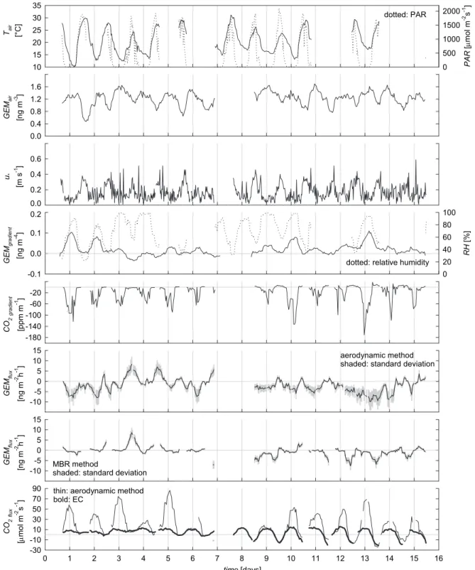
Fig. 1. Time series of measurements at Fruebuel. From top to bottom: air temperature (Tair), photosynthetically active radiation (PAR),

atmospheric GEM concentration at 1.7 m above ground (GEMair), friction velocity (u∗), GEM gradients and relative humidity, CO2

G

E

Mfl

u

x

[n

g

m

-2 h -1 ]

-10 -5 0 5 10 15

G

E

Ma

ir

[n

g

m

-3 ]

0.0 0.4 0.8 1.2 1.6 Ta

ir

[°C]

10 15 20 25 30 35

P

AR

[

µ

m

o

l

m

-2 s -1 ]

0 500 1000 1500 2000

time [days]

0 1 2 3 4 5 6 7 8 9 10 11 12 13 14 15 16

C

O2

fl

u

x

[

µ

m

o

l

m

-2 s -1 ]

-30 -10 10 30 50 70 90

G

E

Mg

ra

d

ie

n

t

[n

g

m

-4 ]

-0.1 0.0 0.1 0.2

R

H

[%

]

0 20 40 60 80 100 u*

[m

s

-1 ]

0.0 0.2 0.4 0.6

thin: aerodynamic method bold: EC

C

O2

g

ra

d

ie

n

t

[p

p

m

m

-1 ]

-180 -140 -100 -60 -20

dotted: relative humidity

G

E

Mfl

u

x

[n

g

m

-2 h -1 ]

-10 -5 0 5 10 15

aerodynamic method shaded: standard deviation

MBR method

shaded: standard deviation

dotted: PAR

G

E

Mfl

u

x

[n

g

m

-2 h -1 ]

-5 0 5 10 15

G

E

Ma

ir

[n

g

m

-3 ]

0 1 2 3 4

Ta

ir

[°C]

10 15 20 25 30 35

P

AR

[

µ

m

o

l

m

-2 s -1 ]

0 500 1000 1500 2000

time [days]

0 1 2 3 4 5 6 7 8 9 10 11 12 13

C

O2

fl

u

x

[

µ

m

o

l

m

-2 s -1 ]

-20 0 20 40 60

G

E

Mg

ra

d

ie

n

t

[n

g

m

-4 ]

-0.2 -0.1 0.0 0.1

S

W

C

[%

-v

o

l]

38 42 46 50

u*

[m

s

-1 ]

0.0 0.2 0.4 0.6

thin: aerodynamic method bold: EC

C

O2

g

ra

d

ie

n

t

[p

p

m

m

-1 ]

-350 -250 -150 -50 50

dotted: soil water content

G

E

Mfl

u

x

[n

g

m

-2 h -1 ]

-5 0 5 10 15

aerodynamic method shaded: standard deviation

MBR method

shaded: standard deviation

dotted: PAR

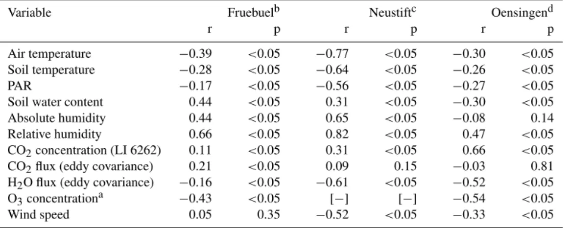
Table 2.Correlation of GEM concentration with meteorological variables.

Variable Fruebuelb Neustiftc Oensingend

r p r p r p

Air temperature −0.39 <0.05 −0.77 <0.05 −0.30 <0.05 Soil temperature −0.28 <0.05 −0.64 <0.05 −0.26 <0.05 PAR −0.17 <0.05 −0.56 <0.05 −0.27 <0.05 Soil water content 0.44 <0.05 0.31 <0.05 −0.30 <0.05 Absolute humidity 0.44 <0.05 0.65 <0.05 −0.08 0.14 Relative humidity 0.66 <0.05 0.82 <0.05 0.47 <0.05 CO2concentration (LI 6262) 0.11 <0.05 0.31 <0.05 0.66 <0.05

CO2flux (eddy covariance) 0.21 <0.05 0.09 0.15 −0.03 0.81

H2O flux (eddy covariance) −0.16 <0.05 −0.61 <0.05 −0.52 <0.05

O3concentrationa −0.43 <0.05 [−] [−] −0.54 <0.05

Wind speed 0.05 0.35 −0.52 <0.05 −0.33 <0.05

a_{data from nearest national monitoring station;}b_N=255–390;c_N=194–375;d_N=31–337

3.3 Atmospheric GEM concentrations

Average atmospheric GEM concentrations measured 1.7 m above ground were 1.2±_{0.2 ng m}−3_{at both, the Fruebuel and}

Neustift sites, and 1.7±_{0.5 ng m}−3_{at the site in Oensingen}

(see Table 1). The highest concentration was measured in Oensingen during daytime with 4.7 ng m−3, the lowest in Neustift with 0.5 ng m−3during the night (see Fig. 1 to 3). As can be seen in Fig. 4 the concentrations in Neustift and Oensingen followed a distinct diurnal pattern with lowest GEM concentrations in the afternoon between 14 and 15 h. This pattern was particularly pronounced in Neustift with an average diurnal amplitude of 0.32 ng m−3. In contrast, a di-urnal signal at Fruebuel was absent and concentrations nearly constant.

Calculation of the correlation coefficients between am-bient GEM concentration and meteorological variables re-vealed moderate linear relationships with relative humidity and atmospheric O3at Fruebuel and Oensingen (see Table 2).

More pronounced correlations of GEM concentration were detected in Neusitft for most variables, notably air tempera-ture and PAR, but no O3record was available for this site.

3.4 CO2and GEM fluxes

In Table 1 a summary of the average GEM and CO2

gradi-ents and fluxes is given for the investigated sites; the corre-sponding time series are shown in Fig. 1 to 3. Due to large spread, fluxes and GEM gradients were smoothed with a 7-point moving average (which corresponds to an interval of

∼_{8 h). As expected, the vertical concentration gradients and}

fluxes of CO2 varied substantially between day and night.

While the highest average day-time gradient (9–15 h) was recorded at Fruebuel with 9.3 ppm m−1, the highest average night-time gradient (23–5 h) was measured in Neustift with

hour of day

11 13 15 17 19 21 23

G

E

Ma

ir

[

n

g

m

-3 ]

0.6 0.8 1.0 1.2 1.4 1.6 1.8 2.0 2.2 2.4

Oensingen Fruebuel Neustift

1 3 5 7 9

Fig. 4. Diurnal trend of atmospheric GEM concentrations at the

three study sites. Shown are hourly mean and standard errors of all measurement days (Fruebuel 14 days, Neustift 16 days, Oensingen 11 days).

−_{43 ppm m}−1_{. The largest gradient of}−_{220 ppm m}−1_was

measured at Oensingen during one night.

As mentioned in the experimental section CO2fluxes were

determined two-fold, with eddy covariance and the aerody-namic method. The former yielded on average a net uptake or deposition of 6.4µmol m−2s−1and 5.3µmol m−2s−1at Fruebuel and Oensingen, respectively, and a mean net CO2

Over the two-week period at Fruebuel CO2fluxes showed a

linear trend towards higher deposition rates.

At all three sites GEM gradients showed a diurnal pattern, which was more pronounced at Fruebuel than at Neustift and Oensingen. Gradients were extremely small with a max-imum value of 0.40 ng m−3m−1 at Oensingen. Average day-time gradients reached 0.02 ng m−3m−1at Fruebuel and were below the minimum resolvable gradient at Neustift and Oensingen. With 0.06 ng m−3m−1the mean night-time gra-dient was highest at Fruebuel; for Neustift and Oensingen mean values of 0.02 and−_{0.04 ng m}−3_m−1_{were calculated.}

At Neustift and Fruebuel night-time gradients were highest in the early morning around 05:00 a.m. In contrast, night-time gradients at Oensingen were negative between measurement days 6 and 10, and peaked before midnight. Figure 1 also shows, that the amplitude of the GEM gradient at Fruebuel increased over time.

Computation of the fluxes yielded on average a small deposition of GEM at Fruebuel and Neustift and slight emission in Oensingen. At Fruebuel, the average GEM fluxes determined by the MBR method and the aerodynamic method were−_{1.6 and}−_{4.3 ng m}−2_h−1_{, respectively. The}

corresponding exchange rates in Neustift were −_{0.5 and} −_{2.1 ng m}−2_h−1_{and in Oensingen 0.3 and 0.2 ng m}−2_h−1_.

The latter two values as well as the exchange rate deter-mined by MBR at Neustift were not significantly different from zero. The highest variability of the fluxes was recorded for Neustift with a range of−_{76 to 37 ng m}−2_h−1_,

deter-mined with the aerodynamic method. At Fruebuel fluctua-tions were smallest with a range of−_{14 to 14 ng m}−2_h−1_,

again determined with the aerodynamic method. Average deposition velocities (vd= −FGEM/cGEM) for Fruebuel and

Neustift were calculated to be 0.04 and 0.01 cm s−1 for the MBR method as well as 0.10 and 0.05 cm s−1for the aero-dynamic method. A linear trend of the GEM flux overlaid by a diurnal pattern with increasing amplitude was observed at Fruebuel. No such trend existed at Neustift and Oensingen and diurnal fluctuations were only visible during some peri-ods and were more pronounced by the aerodynamic method.

4 Discussion

4.1 Evaluation of micrometeorological methods

As every micrometeorological method, flux-gradient tech-niques have certain limitations. One constraint is the foot-print that depends on the prevailing atmospheric conditions, site heterogeneity and measurement height. When measur-ing gradients, the fetch of an upper samplmeasur-ing height is greater than the one at a lower sampling height and therefore gener-ates some uncertainty. A further error is introduced by mea-suring in the so-called roughness sublayer, the region adja-cent to the vegetation, that is directly affected by the grow-ing plants. In this zone common flux-gradient relationships

become progressively less reliable as the gradient measure-ments approach the vegetated surface (Raupach and Legg, 1984; Baldocchi, 2006). For some periods this uncertainty had to be accepted in our study, as the measurements ran autonomously and the sampling lines could not be adjusted to the growing vegetation. Overall, errors associated with the aerodynamic method range between 10 and 30% and are greatest during periods with little turbulence (Baldocchi et al., 1988). Additionally, the MBR method assumes that the transport processes are identical for both species, i.e. GEM and CO2(Lenschow, 1995). In the roughness sublayer this

assumption is not guaranteed and might be another source of uncertainty.

In general, the MBR method yielded smaller average fluxes than the aerodynamic technique and on shorter time scales fluxes often differed considerably. The discrepancies of the averaged fluxes are likely to be of methodological na-ture as the methods differ in the way how they use the gradi-ents to obtain the fluxes. While the aerodynamic method uses universal, empirical relationships to correct for atmospheric stability, the MBR approach relies on the accurate flux deter-mination of the surrogate scalar by an independent method. The short-term fluctuations on the other hand are primarily the result of non-synchronous concentration measurements at the various heights as well as the rather low instrumental resolution of one flux value per 50 min and the small GEM gradients, which were around the minimum resolvable gra-dient of 0.02 ng m−3.

To evaluate the quality of the GEM fluxes, CO2exchange

rates were also estimated with the aerodynamic method and compared to the EC CO2 fluxes. Figures 1 and 2

illus-trate that during some periods the aerodynamic technique strongly overestimated night-time fluxes relative to the EC method. In the stable nocturnal boundary layer, whenu∗is small (<0.1 m s−1), turbulent exchange is inhibited and ver-tical concentration gradients increase. Moreover, the aero-dynamic method is based on the momentum flux equation as well as the wind speed/gradient relationship and requires some empirical formulae to describe atmospheric stability (Baldocchi et al., 1988). Uncertainties in these stability func-tions result in erroneous flux estimates for condifunc-tions of low turbulence (this limitation also applies to the GEM fluxes).

At Fruebuel we also obtained enhanced CO2fluxes by the

aerodynamic gradient method during the day. This overesti-mation relative to the EC method might indicate that the gra-dient was measured too close to the vegetation cover when the grass grew closer to the lower sampling lines. Within and adjacent to the plant cover the universal flux-gradient relationships are no longer valid. Two additional problems may contribute to the observed discrepancy of the measured fluxes: I) When measuring gradients too close to the canopy, sources and sinks of CO2 may not be equal any more and

time [days]

0 1 2 3 4 5 6 7 8 9 10 11 12 13 14

G

E

M

a

ir

[n

g

m

-3 ]

0.8 1.2 1.6 2.0

O

3

[

µ

g

m

-3 ]

-50

0 50

100

150

200 Fruebuel

time [days]

0 1 2 3 4 5 6 7 8 9 10 11 12 13

0 1 2 3 4

5 -50

0

50

100 150

200 solid: TGM

dotted: O₃

Oensingen

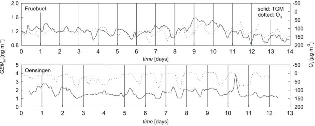
Fig. 5.Time series of atmospheric GEM and ozone concentrations (O₃) at Fruebuel and Oensingen. GEM concentrations were filtered by a

3-point moving average. Oneµg m−3of O3corresponds to 0.5 ppb.

by MBR, as this method uses the ratio of the GEM and CO2

gradients and appears thus more robust. However, due to complex vertical distributions of sources and sinks of trace gases within terrestrial ecosystems, the theoretical basis for the MBR method may be generally questioned. Yet, there are several examples in the literature (e.g. Doskey et al., 2004; Muller et al., 1993; Walker et al., 2006) which have shown that despite this shortcoming, the MBR yields sensible, un-biased flux estimates.

The comparison presented in our manuscript suggests that the aerodynamic method yields more reliable GEM fluxes than the MBR method. This may actually be due to the fact that during daytime conditions the net flux of CO2– the

sur-rogate scalar of the MBR method – is dominated by plant photosynthesis (uptake of CO2 from the atmosphere),

ob-scuring the release of CO2from the soil surface. As the soil

is thought to represent the major source of GEM this would clearly invalidate the theoretical basis of the MBR method. 4.2 Atmospheric GEM concentrations

The mean global GEM concentration is reported to be around 1.7 ng m−3 (Valente et al., 2007). In Europe Munthe and W¨angberg (2001) measured concentrations of 1.34 ng m−3 at Pallas in Finnland and Kim et al. (2005) 1.55 ng m−3at Mace Head in Ireland. The average concentrations of 1.20 to 1.66 ng m−3that we measured at our sites are consistent with these observations.

Moderate correlations of GEM concentration with atmo-spheric O3and relative humidity were detected at Fruebuel

and Oensingen (see Table 1 and Fig. 5). These correlations and the diurnal patterns of GEM and O3support the notion

that O3is an effective reactant to remove Hg0from the

atmo-sphere (Hall, 1995). Additionally, hydroxyl radicals, which have the power to oxidise Hg0 (Lin and Pehkonen, 1999)

and which are formed by the reaction of water vapour with photolysed ozone, may explain our observed correlation with relative humidity. However, our results do not provide clear evidence that oxidation by O3or hydroxyl radicals is

respon-sible for the observed GEM depletion.

4.3 GEM exchange between atmosphere and grassland With average GEM gradients between 0.02 and 0.06 ng m−3m−1, ranging from −_{0.40 to 0.27 ng m}−3_m−1

our results are comparable to gradients measured in other ecosystems. For example, Lindberg and Meyers (2001) measured GEM gradients of 0.03±0.03 ng m−3m−1 over wetland vegetation, Kim et al. (1995) determined values of −0.16 to 0.32 ng m−3 (over 1.4 m) above forest soils in eastern Tennessee and Lindberg et al. (1998) measured gradients of−_{0.091 to 0.064 ng m}−3_m−1_{over forest soils in}

Sweden.

Although the GEM fluxes varied rather strongly, small but statistically significant net deposition rates could be observed at Fruebuel and Neustift. Similar exchange rates – but with inconsistent flux directions – have been estimated for var-ious ecosystems. For example, Obrist et al. (2006) mea-sured a mean deposition rate of 0.2 ng m−2h−1 at another montane grassland site in Switzerland. In Canada Schroeder et al. (2005) observed fluxes between−0.4 to 2.2 ng m−2h−1 over forest soils and 1.1 to 2.9 ng m−2h−1over agricultural fields. Values between−2.2 ng m−2h−1and 7.5 ng m−2h−1 were also measured for forest soils by Kim et al. (1995), and Ericksen et al. (2006) determined a mean emission of 0.9±_{0.2 ng m}−2_h−1_{from different background soils across}

emissions of 50 ng m−2h−1 from contaminated forest soils and Cobos et al. (2002) who measured fluxes of−91.7 to 9.67 ng m−2h−1over an agricultural soil. Different methods were used in these studies and might explain some of the di-vergence between the findings. However, fluxes measured by our group at four different sites (Obrist et al., 2006, this study) indicate net deposition of GEM and imply that grass-lands of the temperate montane climate belt are small net sinks for atmospheric mercury.

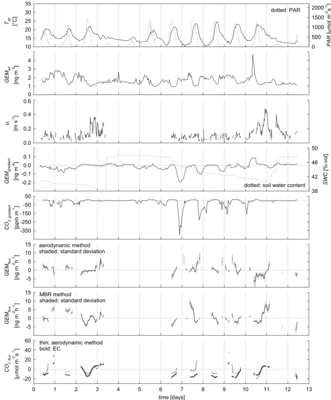
Other than at Fruebuel and Neustift our methods yielded no net flux in Oensingen. This discrepancy might be at-tributed to natural variability, as the observed background fluxes are already extremely low. However, during a pe-riod of three days, negative night-time GEM gradients were observed, indicating emission of mercury (due to low wind speeds no GEM fluxes could be determined; see Fig. 3). Heavy showers during thunderstorms between days 4 and 6 increased the soil water content by approx. 25%, which started to drop again during day six. It appears that the ob-served GEM gradients during this period are linked to the shift in soil moisture. On the other hand, it is also plausi-ble that this pattern resulted from advection of low GEM-containing air that may be associated with the insufficient fetch of this site during night-times.

At Fruebuel and Neustift night-time GEM gradients fol-lowed the pattern of relative humidity. Therefore, we sug-gest that during the night GEM was co-deposited with water condensing on the vegetation surfaces. Although incorpora-tion of mercury into the plant material is conceivable, GEM was eventually re-emitted from the plant surface in the morn-ing when temperature increased and water evaporated again. This re-emission might take place at a fast rate during a short interval that is not resolvable with our measurement tech-nique.

A linear trend of the GEM flux could be observed at Frue-buel, resulting from the growing vegetation after a grass cut at the beginning of the campaign. In part this trend is arti-ficial as the growing grass increases the atmospheric rough-ness sublayer, thereby reducing turbulence and enhancing the GEM gradients. However, with increasing plant surface area more GEM may be adsorbed by vegetation and adds to the positive gradients. The unbiased part of the trend is reflected in the CO2flux estimated by EC, the method that is

indepen-dent of gradients measurements. In Neustift, where the grass was also cut at the start of the measurement campaign, no such trend was visible. The flux signal rather seems to have a component with a periodicity of 4 to 5 days that conceals any long-term trend. Further investigations would be required at this site to ascertain the processes resulting in this signal.

5 Conclusions

In order to estimate air-surface GEM fluxes of uncontami-nated grasslands along the Swiss and Austrian Alps we ap-plied two micrometeorological methods. Both, the aerody-namic and the MBR methods proved suitable to estimate net exchange rates on time scales of a few hours and longer. Due to the required pre-concentration technique for the detection of GEM, fluxes could not be resolved sufficiently on shorter time scales.

With respect to gaseous exchange our results suggest that grasslands of the temperate montane climate are a net sink for atmospheric mercury. This sink is very small com-pared to emissions of contaminated and naturally enriched areas (these are in the order of 100 to>1000 ng m−2_h−1_).

Nonetheless, deposition could add significant quantities of mercury to remote terrestrial ecosystems if these fluxes are confirmed in other locations. On the condition that deposited mercury is stably bound in the pedosphere, this would also entail a long-term reduction in atmospheric mercury.

At two of our sites we observed day-time depletion of GEM, which may be attributed to the oxidation of GEM by O3 and other reactive trace gases. However, no clear

cause and effect relationship could be determined. On the other hand, night-time deposition of GEM was measured fre-quently and seems to be the result of co-precipitation with condensing water.

Acknowledgements. We thank the Swiss National Science Foun-dation (project numbers: 200020-113327/1 to D. Obrist and C. Alewell; 200021-105949 to W. Eugster and R. A. Werner) and the Austrian National Science Foundation (project number: P17560-B03 to Georg Wohlfahrt) for financing this project and would like to express our appreciation to F. Conen, W. Eugster and R. Vogt for their valuable help in experimental and micrometeoro-logical issues.

Edited by: A. Hofzumahaus

References

Baldocchi, D.: Advanced topics in biometeorology and microm-eteorology: Lecture on micrometeorological flux measurement methods, http://nature.berkeley.edu/biometlab/espm228/, 2006. Baldocchi, D., Hicks, B. B., and Meyers, T. P.: Measuring

biosphere-atmosphere exchanges of biologically related gases with micrometeorological methods, Ecology, 69, 1331–1340, 1988.

Cobos, D. R., Baker, J. M., and Nater, E. A.: Conditional sampling for measuring mercury vapor fluxes, Atmos. Environ., 36, 4309– 4321, 2002.

Dabberdt, W. F., Lenschow, D. H., Horst, T. W., Zimmerman, P. R., Oncley, S. P., and Delany, A. C.: Atmosphere-Surface Exchange Measurements, Science, 260, 1472–1481, 1993.

Doskey, P. V., Kotamarthi, V. R., Fukui, Y., Cook, D. R., Breitbeil, F. W., and Wesely, M. L.: Air-surface exchange of peroxyacetyl nitrate at a grassland site, J. Geophys. Res.-Atmos., 109, 2004. Du, S. H. and Fang, S. C.: Uptake of Elemental Mercury-Vapor by

C3-Species and C4-Species, Environ. Exp. Bot., 22, 437–443, 1982.

Edwards, G. C., Rasmussen, P. E., Schroeder, W. H., Wallace, D. M., Halfpenny-Mitchell, L., Dias, G. M., Kemp, R. J., and Ausma, S.: Development and evaluation of a sampling system to determine gaseous Mercury fluxes using an aerodynamic mi-crometeorological gradient method, J. Geophys. Res.-Atmos., 110, D10306, doi:10.1029/2004JD005187, 2005.

Ericksen, J. A., Gustin, M. S., Xin, M., Weisberg, P. J., and Fernan-dez, G. C. J.: Air-soil exchange of mercury from background soils in the United States, Sci. Total Environ., 366, 851–863, 2006.

Fay, L. and Gustin, M.: Assessing the influence of different atmo-spheric and soil mercury concentrations on foliar mercury con-centrations in a controlled environment, Water Air Soil Poll., 181, 373–384, 2007.

Foken, T.: Angewandte Meteorologie: mikrometeorologische Methoden, Springer, Berlin, 2006.

Fritsche, J., Obrist, D., Zeeman, M., Conen, F., Eugster, W., and Alewell, C.: Elemental mercury fluxes over a sub-alpine grass-land determined with two micrometeorological methods, Atmos. Environ., 42, 2922–2933, 2008.

Gustin, M. S. and Lindberg, S. E.: Terrestrial mercury fluxes: is the net exchange up, down, or neither?, in: Dynamics of mercury pollution on regional and global scales, edited by: Pirrone, N. and Mahaffey, K. R., Springer, New York, 241–259, 2005. Hall, B.: The Gas-Phase Oxidation of Elemental Mercury by

Ozone, Water Air Soil Poll., 80, 301–315, 1995.

IOMC: Global Mercury Assessment, Tech. rep., UNEP Chemicals, Geneva, 2002.

Keeler, G. J. and Landis, M. S.: Standard operating procedure for sampling vapor phase mercury, http://www.epa.gov/grtlakes/ lmmb/methods/, 1994.

Kim, K. H., Lindberg, S. E., and Meyers, T. P.: Micrometeorolog-ical Measurements of Mercury-Vapor Fluxes over Background Forest Soils in Eastern Tennessee, Atmos. Environ., 29, 267– 282, 1995.

Kim, K.-H., Ebinghaus, R., Schroeder, W. H., Blanchard, P., Kock, H. H., Steffen, A., Froude, F. A., Kim, M.-Y., Hong, S., and Kim, J.-H.: Atmospheric Mercury Concentrations from Several Observatory Sites in the Northern Hemisphere, J. Atmos. Chem., 50, 1–24, 2005.

Kljun, N., Kastner-Klein, P., Fedorovich, E., and Rotach, M. W.: Evaluation of Lagrangian Footprint Model Using Data from Wind Tunnel Convective Boundary Layer, Agric. For. Meteorol., 127, 189–201, 2004.

Kormann, R. and Meixner, F. X.: An Analytical Footprint Model for Non-Neutral Stratification, Boundary-Layer Meteorol., 99, 207– 224, 2001.

Lenschow, D.: Micrometeorological techniques for measuring biosphere-atmosphere trace gas exchange, in: Biogenic trace gases: measuring emissions from soil and water, edited by: Mat-son, P. and Harriss, R., Blackwell Science Ltd, Cambridge, 126– 163, 1995.

Lin, C. J. and Pehkonen, S. O.: The chemistry of atmospheric mer-cury: a review, Atmos. Environ., 33, 2067–2079, 1999. Lindberg, S. and Meyers, T.: Development of an automated

mi-crometeorological method for measuring the emission of mer-cury vapor from wetland vegetation, Wetl. Ecol. Manag., 9, 333– 347, 2001.

Lindberg, S., Vette, A., Miles, C., and Schaedlich, F.: Mercury speciation in natural waters: Measurement of dissolved gaseous mercury with a field analyzer, Biogeochemistry, 48, 237–259, 2000.

Lindberg, S. E., Meyers, T. P., Taylor, G. E., Turner, R., and Schroeder, W.: Atmoshere-surface exchange of mercury in a for-est: Results of modeling and gradient approaches, J. Geophys. Res.-Atmos., 97, 2519–2528, 1992.

Lindberg, S. E., Kim, K. H., Meyers, T. P., and Owens, J. G.: Micrometeorological Gradient Approach for Quantifying Air-Surface Exchange of Mercury-Vapor – Tests over Contaminated Soils, Environ. Sci. Technol., 29, 126–135, 1995.

Lindberg, S. E., Hanson, P. J., Meyers, T. P., and Kim, K. H.: Air/surface exchange of mercury vapor over forests – The need for a reassessment of continental biogenic emissions, Atmos. En-viron., 32, 895–908, 1998.

Lindberg, S. E., Ebinghaus, R., Engstrom, D., Feng, X., Fitzgerald, W. F., Pirrone, N., Prestbo, E., and Seigneur, C.: A Synthesis of Progress and Uncertainties in Attributing the Sources of Mercury in Deposition, Ambio, 36, 19–33, 2007.

Meyers, T. P., Hall, M. E., Lindberg, S. E., and Kim, K.: Use of the modified Bowen-ratio technique to measure fluxes of trace gases, Atmos. Environ., 30, 3321–3329, 1996.

Millhollen, A., Obrist, D., and Gustin, M.: Mercury accumulation in grass and forb species as a function of atmospheric carbon dioxide concentrations and mercury exposures in air and soil, Chemosphere, 65, 889–897, 2006.

Muller, H., Kramm, G., Meixner, F., Dollard, G. J., Fowler, D., Pos-sanzini, M.: Determination of HNO₃Dry Deposition by Modi-fied Bowen-Ratio and Aerodynamic Profile Techniques, Tellus B, 45, 346–367, 1993.

Munthe, J. and W¨angberg, I.: Atmospheric Mercury in Sweden, Northern Finland and Northern Europe, Tech. rep., IVL Swedish Environmental Research Institute, Gothenburg, 2001.

Obrist, D.: Atmospheric mercury pollution due to losses of terres-trial carbon pools?, Biogeochemistry, 85, 119–123, 2007. Obrist, D., Conen, F., Vogt, R., Siegwolf, R., and Alewell, C.:

Esti-mation of Hg0exchange between ecosystems and the atmosphere using222Rn and Hg0concentration changes in the stable noctur-nal boundary layer, Atmos. Environ., 40, 856–866, 2006. Pirrone, N. and Mahaffey, K. R.: Where we stand on mercury

pol-lution and its health effects on regional and global scales, in: Dy-namics of mercury pollution on regional and global scales, edited by: Pirrone, N. and Mahaffey, K. R., 1–21, Springer, New York, 2005.

Poissant, L. and Casimir, A.: Water-air and soil-air exchange rate of total gaseous mercury measured at background sites, Atmos. Environ., 32, 883–893, 1998.

Raupach, M. R. and Legg, B. J.: The uses and limitations of flux-gradient relationships in micrometeorology, Agr. Water Manage., 8, 119–131, 1984.

Banic, C. M.: Gaseous mercury emissions from natural sources in Canadian landscapes, J. Geophys. Res., 110(D18), D18302, doi:10.1029/2004JD005699, 2005.

Valente, R., Shea, C., Humes, K., and Tanner, R.: Atmospheric mercury in the Great Smoky Mountains compared to regional and global levels, Atmos. Environ., 41, 1861–1873, 2007.

Walker, J. T., Robarge, W. P., Wu, Y., and Meyers, T. P.: Mea-surement of bi-directional ammonia fluxes over soybean using the modified Bowen-ratio technique, Agr. Forest Meteorol., 138, 54–68, 2006.