A method to elicit beliefs as most likely intervals
Karl H. Schlag
∗Joël J. van der Weele
†Abstract
We show how to elicit the beliefs of an expert in the form of a “most likely interval”, a set of future outcomes that are deemed more likely than any other outcome. Our method, called the Most Likely Interval elicitation rule (MLI), asks the expert for an interval and pays according to how well the answer compares to the actual outcome. We show that the MLI performs well in economic experiments, and satisfies a number of desirable theoretical properties such as robustness to the risk preferences of the expert.
Keywords: Belief elicitation, scoring rules, subjective probabilities, confidence intervals.
1
Introduction
In many instances, uncertainty about future events is the main obstacle to making good decisions. To reduce uncer-tainty, people frequently consult others who have different or superior information. The consultation may concern to-morrow’s temperature, future market conditions, an interest rate or stock price, or the actions of a politician or business competitor.
We propose a novel method for how to get information from an expert in the form of an interval. Intervals have the the advantage that one need not commit to a specific number nor deal with complex mathematical objects (Mahieu et al., 2014). Moreover, reporting an interval gives the expert the opportunity to provide information about the location of her beliefs and her uncertainty at the same time. Our method relies on monetary incentives. We propose to pay the expert based on the width of the specified interval and whether or not the unknown outcome lies in the interval. These incen-tives give the expert a reason to think well about her report and allows, given standard assumptions on the expert’s de-cision making process, to make inferences about her beliefs. Our payment method incentivizes of the expert to select a “most likely interval”, where any event inside the interval is at least as likely to occur as any event outside the interval. It features an adjustable parameter to influence the width of the reported interval. The inferences from our method are valid for all degrees of risk aversion of the expert, un-like existing elicitation methods (Winkler & Murphy, 1979;
We would like to thank the editor, Jon Baron, an anonymous referee and diverse seminar participants for useful comments.
Copyright: © 2015. The authors license this article under the terms of the Creative Commons Attribution 3.0 License.
∗University of Vienna, Vienna. E-mail: [email protected] †Corresponding author. University of Amsterdam. Email:
[email protected]. Tel. +31 (0)20 5254213. Address: CREED, Department of Economics, University of Amsterdam, Roeterstraat 11, 1018WB Ams-terdam, the Netherlands.
Schmalensee, 1976). We show that our scoring rule per-forms well in laboratory experiments and satisfies several theoretical desiderata.
We now introduce our method in more detail in the con-text of an example. Suppose a company wants to know what an expert thinks the price of crude oil will be in the next month. The company may ask for a single price estimate, for example the expert’s understanding of the mean, median or modal price. However, a point estimate of the crude oil price provides no information on risk or dispersion, which is vital for contingency planning. At the opposite extreme one may wish to get a complete understanding of the expert’s be-liefs and ask for the likelihood of each possible price level (Matheson & Winkler, 1976; Harrison et al., 2013a). While this provides maximal information, it is a time-consuming way to elicit beliefs and presupposes fluency with the math-ematical concept of a probability distribution.
An attractive and tractable alternative is to ask the expert for the prices for next month that she regards as being most likely. These prices could be few or many, concentrated or widely dispersed. It seems is reasonable to assume, as we will do in this paper, that the most likely prices are concen-trated around some value (i.e. the mode), which means they can be elicited as an interval.1 Our elicitation method asks
for a lower and upper bound of the likely price level, and pays the expert only if the realized price lies in the inter-val. The reward is a function of the width of the interval, and does not depend on the end points. This implies that the expert has an incentive to specify an interval that contains only the most likely prices, which is why we call our rule the Most Likely Interval elicitation rule (MLI).
Apart from capturing most likely price levels, the com-pany may want to vary the precision of the report. For in-stance, suppose that company profits are not very sensitive to price deviations and all the company cares about is some
1For other cases where we think that most likely prices will be disjoint
we present a method for eliciting most likely sets.
indication of the likely outcome. In this case, obtaining a narrow interval with some highly likely events may be op-timal even if this means a relatively low confidence that the price will fall in the interval. By contrast, if the company wants to assess the likelihood of an extreme price change, it may prefer to obtain an wide interval with a high degree of confidence.
To address these trade-offs, our elicitation method fea-tures a parameterγthat can be chosen freely, and regulates how much the expert is punished for specifying a wide inter-val. Increasing this penalty will result in a smaller reported set of most likely events and thus will decrease the confi-dence of the expert that the price will obtain in the specified range. Using a formal model of how the expert makes de-cisions (i.e. subjective expected utility maximization) we designed the MLI such that each expert will include at least a mass ofγ in the interval. We therefore refer toγas the minimal confidence level.
In order to discipline the expert not to present an inter-val that is too large, we need to quantify what large means. To this end, we assume bounds on the range of potential outcomes, and the MLI punishes the width as a fraction of this range. For example, when the outcome of interest is a percentage then the natural range is from0 to100. In the crude oil example, where these bounds are not given by the problem itself, one can choose the range such that historical observations falls well within them, like1and200US$ per barrel.
To summarize, our rule guarantees from any expert who maximizes expected utility, that the reported interval only contains those events that the expert thinks are most likely to occur and have a minimal confidence of γ. The actual degree of confidence may be larger than γ,depending on the degree risk aversion of the expert. More risk averse ex-perts will tend to submit larger intervals to guarantee a pos-itive payoff. In principle, one could try to counter act this tendency, with the aim to elicit an interval with confidence close toγ, by designing a different rule for each expert. In most applications there is not enough information about the expert to do so. Therefore, our rule is designed to capture at least confidenceγfor any risk averse or risk neutral ex-pert. Experimental evidence indicates that the large majority of people are either risk averse or risk neutral (e.g. Holt & Laury, 2002).
The theoretical research on interval elicitation has fo-cussed on obtaining an interval with a pre-specified like-lihood, a so-called credible interval (Murphy & Winkler, 1974). However a credible interval itself does not neces-sarily reveal any information on what events are most likely as it can contain many least likely events. In fact, we show that none of the previous interval elicitation rules, presented by Winkler and Murphy (1979) and Schmalensee (1976), elicits most likely events.
In contrast to other papers on interval scoring rules, we
explicitly compare different rules on the basis of their theo-retical properties. Our rule is more generally applicable than existing scoring rules, as it is designed for experts that are either risk neutral or risk averse. In contrast, most of the isting literature on scoring rules focuses on risk neutral ex-perts. Elicitation mechanisms that generalize to all risk pref-erences exist, but only for means and probabilities (Schlag et al., 2015). Moreover, these mechanisms are substantially more complicated than our interval rule as they require ei-ther randomized payoffs (Hossain & Okui, 2013; Schlag & Van der Weele, 2013) or additional elicitations (Offerman et al., 2009), and there is an open debate about the empir-ical performance of such mechanisms (Selten et al., 1999; Harrison et al., 2013b).
Finally, the empirical research on confidence interval elic-itation relies mostly on unincentivized elicelic-itation methods, or ad-hoc scoring rules. For example, Cesarini et al. (2006) reward the subjects if they correctly estimate the hit rate of their previously stated intervals. Blavatskyy (2008) shows that this method is easy to game. Other studies (e.g. Bude-scu & Du. 2007) simply reward subjects proportional to their accuracy rate, which can be gamed by simply report-ing very large intervals regardless of beliefs. The underuse of appropriate incentives is unfortunate, as there is evidence that experimental subjects may be naturally inclined to re-port different confidence levels than those requested by the experimenter (Yaniv & Foster, 1997), and that appropriate incentives improve accuracy of forecasts (Krawczyk, 2011). This article proceeds as follows. The next section intro-duces the elicitation environment and the MLI. Sections 3 and 4 provide examples of how to implement the rule and discuss potential applications. Section 5 provides a more formal discussion of the properties of the MLI, and Section 6 compares those properties to those of other scoring rules in the literature. Section 7 discusses the robustness of the rule to the assumptions we have made, and provides some extensions. Section 8 concludes.
2
The elicitation environment and the
MLI
The Most Likely Interval elicitation rule (MLI) pays the expert for her reported interval whenever the true realiza-tion lies in the interval she submitted, where the payment is strictly decreasing in the width of the reported interval. The rule has a free parameterγ ∈(0,1). The payment received when submitting and interval[L, U]when value xis real-ized is denoted bySM(L, U, x),and depends on the width
W =U−Lof the interval as follows
SM(L, U, x) = (
1− W b−a
g
ifx∈[L, U]
0 ifx /∈[L, U] (1)
where g = 1−γγ. Ifγ = 1/2 then it obtains its simplest, linear form:
SM(L, U, x) = (
1− W
b−a ifx∈[L, U] 0 ifx /∈[L, U].
The properties of the rule are invariant to any affine transfor-mation ofSM. This means that one can regulate the amount
paid out to the expert by multiplying the payoffs with an ap-propriate number. The rule can be applied to any random variableX that has support in [a, b]. In particular, it also applies to transformations ofX, likelog(X)or tocX+d, as long as one transforms the boundariesaandbin the same way.
We designed the MLI to be able to make inferences from the elicited interval about the beliefs of the expert under some assumptions on how the expert makes choices. Sup-pose the beliefs of the expert of a random variable of interest X can be described by the cumulative density functionFX.
We assume these beliefs satisfy the following two assump-tions: (i)FX is a continuous distribution with at most one
mass point and densityf.(ii) FX is single peaked, which
means that the likelihood of an event decreases as one moves away from an event that has the highest likelihood. More formally,Xis single-peaked if there existsx0such thatf is
increasing inxforx≤x0and decreasing inxforx≥x0.
Any valuex0with this property is called a mode ofX.2We
believe the assumption of single-peakedness makes sense under many circumstances. In cases where it does not, the MLI can easily be extended to allow for multiple intervals as outlined in Section 7.
Suppose now that the interval specified by the expert, denoted by [L∗, U∗], is chosen exclusively on the basis of
monetary payoffsSM. Then the expert is best off by
plac-ing an interval with widthW within the range[a, b]where it “covers” or contains the true event with the highest prob-ability. As beliefs are single-peaked, the reported inter-val[L∗, U∗]will contain all values with a likelihood above
some threshold, and thus contains a mode ofX.We refer to this key property as “most likely”.
2Note thatx
0is the only candidate for a point mass so we can letx0
denote the mass point whenever it exists.
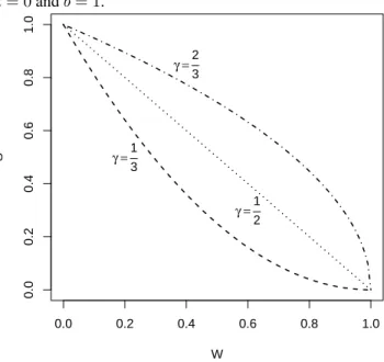
Figure 1: Relation between the widthW(on thex-axis) and paymentSM (on they-axis) for different values ofγand for
a= 0andb= 1.
0.0 0.2 0.4 0.6 0.8 1.0
0.0
0.2
0.4
0.6
0.8
1.0
W
S γ =1
3
γ =2
3
γ =1
2
The widthW∗ =U∗−L∗of the reported interval
con-tains further information about the expert’s uncertainty. To see this, consider the dependency of MLI on the widthW. IncreasingW increases the likelihood of being paid but de-creases the payment itself. For small values ofW,when the expert is very certain about what will happen, an increase in W/(b−a)leads to an decrease in payment approximately equal to−g. In Figure 1, we plot the payment as a function of the widthW of the interval for three cases,g = 1/2,1
and2, so forγ= 2 3,1and
1
3, anda= 0andb= 1.
Asγincreases, andgdecreases, the incentives to increase W become stronger. Whenγ is small then the expert has the highest incentives to report a small interval. Choosing a small value forγcan be of interest when one wishes to ob-tain a point prediction about what is most likely to happen, but one does not wish to force the expert to commit to a spe-cific number. Whenγis large then the interval will tend to be large, and the events that are not included in the interval can be considered ‘extreme’ or unlikely events.
If we assume that the expert is a subjective expected util-ity maximizer with respect to the payoffsSM, we can also
make inferences about the total or joint probability that the realization x will be in the interval. Since the parame-terγ influences the width, it also influences this probabil-ity. In particular, if the expert is either risk neutral or risk averse, the interval will cover at least the massγof the ex-pert’s beliefs, as we will show in Section 5. More formally, PFX(X ∈[L∗, U∗])≥γ.This “coverage” property means
how more dispersed beliefs translate to wider intervals. In this sense the width captures the expert’s degree of uncer-tainty.
To summarize, the MLI can extract information about the expert’s beliefs in terms of location, confidence and degree of uncertainty.
3
Implementation: An example
In this section, we illustrate the implementation of the MLI in an experimental context. To do so, we analyze the exper-iment by Galbiati et al. (2013), in which both co-authors of the current paper were involved and that saw, to our knowl-edge, the first experimental implementation of the MLI.3
Experiment outline. The experimental context was a
strategic game between two players, called the minimum effort game. In this game, both players had to choose an “ effort level”e, which could be any number between110
and170. The payoffs ofπiof playeri = 1,2depended on
the effort of both players as follows
πi(e1, e2) = min(e1, e2)−0.85∗ei. (2)
Thus, each player was rewarded according to the minimum of the two effort levels, while “paying” a cost proportional to her own effort.4
As we explained to the participants in the instructions, it is optimal for each player to match the effort level of the other player. If the own effort level exceeds that of the opponent, one could increase payoffs by decreasing effort. When effort is lower than that of the opponent, one could increase payoffs by increasing efforts.5 Thus, a crucial
de-terminant of a player’s actions is what effort s/he thinks the other player will choose. Moreover, the nature of uncer-tainty about the other’s effort matters, because undershoot-ing the other’s effort is less costly than overshootundershoot-ing it. This makes the MLI a suitable elicitation method. We chose γ = 0.5to maximize the simplicity of the rule, and scaled the payoffs in order to balance them with the earnings from the effort decision.
The subjects played two rounds of this game. The second round was played without feedback about the outcomes of the first round. We consider two experimental conditions of
3The main results presented here regarding the width and the location
of the intervals in different experimental conditions are present in Galbiati et al. (2013). The results concerning the accuracy of beliefs and the relation between beliefs and effort are novel.
4The original experiment featured a third, inactive player who benefitted
from the minimum effort of the other players. For our purposes this player can be ignored.
5As a consequence, all strategy profiles with two equal effort levels are
Nash equilibria. Equilibrium payoffs for both players are higher in Nash equilibria with higher effort levels.
the experiment, which differed only with respect to the de-tails of the second round. In theControlcondition,30 par-ticipants played exactly the same game in the two rounds. In theIncentivecondition, with34participants, we imple-mented a small penalty for deviating from the maximum effort of170. Formally, we added to the payoffs in (2) a component−1
2(170−ei). This implied that higher effort
became more attractive as it became less risky (although still suboptimal) to overshoot the opponent’s effort.
Belief elicitation instructions. Beliefs were elicited in
both rounds of the game, simultaneously with the effort choice. The MLI was introduced to the experimental par-ticipants with the following instructions.
Guessing the other’s choice
We now ask you to make a guess about the number cho-sen by the other player. The guess is made by specify-ing a range (given by its lower boundLand its upper
boundU) in which the other player’s choice is believed
to belong. The earnings in tokens of either player 1 or player 2 from making this guess are determined as follows. A wrong guess (the actual number chosen by the other player falls outside the specified range) yields nothing. A correct guess (the actual number chosen by the other player lies within the specified range) yields 15% of the difference between 60 and the width of the rangeU
−L. Therefore the smaller the specified range,
the higher the earnings if the guess is correct. However, a smaller range also increases the risk that the guess is not correct, in which case no tokens are earned.6
Note that tokens where converted to real money at the end of the experiment.
Results. First, we investigate if effort forecasts elicited
with the MLI were accurate. Note that the MLI elicits in-dividual subjective beliefs that need not conform to the ac-tual frequencies. Nevertheless, we can compare the average elicited interval to the actual distribution to understand how well-calibrated the subjects are on an aggregated level.
Figure 2 shows the actual frequency distribution of effort in theIncentivecondition (light/red line) and to theControl (black line), which present the “right” answer for subjects to estimate. In line with the theoretical predictions spelled out in Galbiati et al. (2013), the distribution of effort in-deed went up in theIncentivecondition relative to the Con-trol. The shaded areas in Figure 2 show the average intervals
6In addition, a more mathematical presentation was provided but not
read out loud by the experimenter. If the numberZchosen by the other player lies in the range (it is greater than or equal toLand less than or equal toU) then the player who has chosenLandUgets0.15×(60−
Figure 2: Distribution density plots of effort (thick lines) measured in units1ewhereeis effort. The shaded areas rep-resent the corresponding average estimated interval in the IncentiveandControlcondition.
0
.0
1
.0
2
.0
3
D
e
n
si
ty
110 120 130 140 150 160 170 Effort
Effort (Control) Effort (Incentive) Avg. chosen interval
(Control) Avg. chosen interval (Incentive)
specified by the participants in the second round in the dif-ferent conditions. As is clear from the figure, the location of the intervals moved in line with the theoretical predic-tions. What is more, in both cases, the average interval cap-tures the mode of the distribution, and are not very far away from capturing only the most frequent effort levels. From these results it appears that the average intervals are well-calibrated. This is a useful property in applications and sug-gests that aggregated intervals have favorable properties, the theoretical analysis of which we leave to future research.
Second, we investigate the width of the belief interval. The average widths of the chosen interval in the first round was about 18 points, and was actually slightly higher in the Incentivecondition. What interests us most is whether the width of the interval responds to the incentives in the second round of the game. Effort moved up in theIncentive condi-tion and the standard deviacondi-tion of effort declined from 19.4 in theControlto 17.5 in theIncentivecondition. Thus, as ef-fort became more predictable, it is natural to expect that the dispersion of beliefs goes down in theIncentivecondition. As we will show in Section 5, this implies that the optimal interval width declines. Figure 3 shows the change in the mean width of the intervals between the rounds, with 95% confidence intervals. Interval widths remained virtually un-changed in theControlcondition, while they declined sub-stantially (by 26%) in theIncentivecondition.
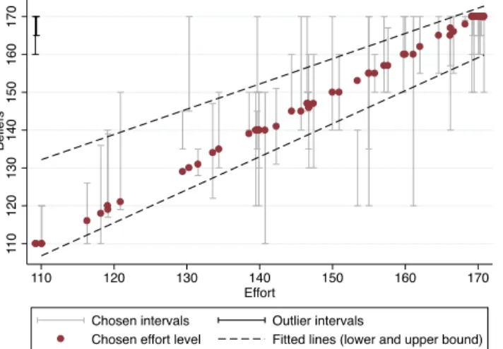
Finally, we investigate the relation between the beliefs and effort that are elicited from the sameperson. Such a connection demonstrates that people act upon their belief, and support the conclusion that we elicited a relevant vari-able. Figure 4 shows the relation between effort (x-axis) and beliefs (y-axis), pooling both experimental conditions. The chosen belief intervals are shown in grey. As is
appar-Figure 3: Change in the average interval width between the first and second round in theIncentiveandControl condi-tion, with 95% confidence intervals.
2
0
-2
-4
-6
-8
-1
0
C
h
a
n
g
e
i
n
i
n
te
rva
l
w
id
th
Control Incentive Experimental condition
Figure 4: This graph shows the relation between effort (x-axis) and beliefs (y-(x-axis), pooling both experimental condi-tions. The chosen belief intervals are shown in grey, except two outliers at the top left, shown in black. The two fitted lines pertain to the upper and lower bound of intervals re-spectively, ignoring the two outliers. Dots indicate the effort choice. These dots do not lie exactly on the 45 degree line as we added some noise to avoid overlays of data points.
1
1
0
1
2
0
1
3
0
1
4
0
1
5
0
1
6
0
1
7
0
Be
lie
fs
110 120 130 140 150 160 170 Effort
Chosen intervals Outlier intervals
Chosen effort level Fitted lines (lower and upper bound)
ent from the black lines fitted to capture the lower and upper bound of the belief interval, higher and more precise beliefs are associated with higher efforts. Moreover, looking at the dots that indicate the actual effort choice, we see that effort is inside the belief interval in most cases. This is what one would expect in this strategic situation where each player has incentive to match the effort level of the other player.
predict the choice of their opponents in a strategic environ-ment. We found that, first, average intervals specified by the participants include the mode of the actual distribution and are not far from capturing the most likely events. Second, both the width and the locations of the intervals respond to our experimental manipulation in a way that was in line with theoretical predictions. Third, there is a robust relationship between the specified beliefs about the opponents and the strategic choices in the experiment. These findings indicate that the MLI is a reliable method to elicit beliefs in this con-text.
4
Applications
In this section we provide an overview of potential applica-tions of the MLI. To do so, we review applicaapplica-tions of MLI in previous experimental work and discuss potential appli-cations in finance, management and other settings.
4.1
Applications in experiments
Based on earlier versions of this paper, the MLI has been implemented in economic experiments to elicit expectations about a diverse set of variables. These experiments demon-strate the flexibility of the MLI both in the type of expec-tation that can be elicited and in the way that the resulting data can be analyzed.
Elicitation has taken place in both strategic and non-strategic settings. As an example of the latter, Peeters and Wolk (2014) use the MLI to elicit repeated forecasts about realizations of a random variable. Examples of strategic set-tings are the use of the MLI to elicit beliefs about contribu-tions to a public good (Cettolin & Riedl, 2013) or a risk shar-ing fund (Tausch et al., 2014). The MLI has also been used to elicit beliefs about characteristics of other experimental participants, such as their beliefs (Peeters et al., 2015) or risk aversion (Cettolin & Riedl, 2015).
When it comes to analysis of the data, some authors use the midpoint of the interval as a measure for the location of beliefs, either as an explanatory variable in regressions (Cettolin & Riedl, 2013; Peeters et al., 2015) or as the ob-ject of non-parametric comparisons to assess the importance of beliefs in different experimental conditions (Tausch et al., 2014; Cettolin & Riedl, 2015). With respect to the width of the interval, Peeters et al. (2015) uncover differences in the uncertainty of participants in different strategic roles. Cet-tolin and Riedl (2013) find a positive correlation between a measure of risk aversion of the participants and their elicited interval width, a correlation which is significant at1%.7 Fi-nally, Peeters and Wolk (2014) demonstrate how to aggre-gate the elicited intervals of multiple individuals and show
7This result is not reported in their papers, but confirmed in personal
correspondence.
that the calibration of forecasts about the realization of a random variable improves with the number of individuals.
One potentially interesting application of the MLI relates to measuring overconfidence with intervals. Countless stud-ies show that 90% confidence intervals elicited without in-centives are accurate much less than 90% of the time (Russo & Schoemaker, 1992; Moore & Healy, 2008). Yaniv and Foster (1997) argue that participants do not necessarily re-port the confidence levels requested by the experimenter, but tend to make their own normative trade-offs between infor-mativeness and accuracy. Appropriate incentives, such as those provided by the MLI could help reduce the miscom-munication between experimenter and participant. Indeed, Krawczyk (2011) shows that providing incentives for truth-ful elicitation improves results. In Section 6, we argue that the MLI may be a good alternative to the incentives used in Krawczyk (2011), although this remains to be tested empir-ically.
4.2
Real world applications
Estimations in the form of intervals play a role in many ap-plications. Perhaps the most salient one is in weather fore-casting, where they are common in forecasts of tempera-tures. Indeed, a literature exists in weather forecasting that investigates the interval reports of weather forecasters (e.g. Hamill & Wilks, 1995). Forecasts of financial variables such as inflation or growth rates are also often given as confidence intervals, since risk plays an important role in financial de-cisions. For instance, trader’s buying and selling strategies depend on corridors in which prices are expected to lie. The MLI can be used to elicit such a corridor, by identifying LandU by parallel lines that have distanceU −L. Cen-tral banks can use the MLI to elicit intervals from economic experts about future unemployment and inflation, and use these estimates construct contingent policies.
Financial officers in businesses can use interval forecasts to plan continent pricing strategies or sales targets. Future prices and sales depend on many factors unknown to man-agers, who could elicit intervals from employees in order to improve the realism of targets. Even current performance may be hard to measure, and could be elicited as interval es-timates from employees. In this context, the free parameter γin the MLI is useful to communicate the desired level of precision. In Section 7 we also explain how, with a small modification, one can also use the MLI to elicit estimates of tail risks, like the common measure Value at Risk.
an expert. Second, while CIs derived from statistical models would contain the outcome with probability equal toγ, the MLI elicits most likely intervals which contain the outcome with probability ofat leastγ.
5
Theoretical properties of the MLI
The previous sections have shown how one can elicit be-liefs using the MLI and informally discussed some of the properties of the elicited interval. In this section, we discuss the theoretical properties of MLI and the associated infer-ences more formally and extensively. Our companion paper (Schlag & Van der Weele, 2014) provides additional discus-sion of the theoretical aspects of these properties. All proofs are contained in the Appendix.
We consider the optimal response of expert endowed with preferences over R that admit an expected utility repre-sentation, denoted by u. An interval scoring rule S is a mapping from [a, b]3 to R+ where S(L, U, x) is the payoff that the expert receives after reporting the inter-val [L, U] and the event x is realized. Let [L∗, U∗] = [L∗(F
X, S, u), U∗(FX, S, u)]denote be the interval
cho-sen by an expert with utility uand beliefsFX when paid
by the rule S. Let W∗(F
X, S, u) = U∗(FX, S, u) −
L∗(FX, S, u) be its width and let M∗(FX, S, u) =
PFX(X ∈[L∗(FX, S, u), U∗(FX, S, u)])be the
probabil-ity that the event belongs to the elicited interval.
The expert’s reported interval depends on her beliefs and risk preferences. Inferences from interval elicitation that depend on the assumption of risk neutrality of the expert should be approached with caution. Holt and Laury (2002) present evidence that most experimental subjects are risk averse. Armantier and Treich (2013) and Offerman et al. (2009) show that most subjects behave as if they are risk averse in the context of belief elicitation. Hence we choose to model the expert as being either risk neutral or risk averse and consider only concaveu.
We first show that an optimal interval always exists.
Proposition 1. For any single-peakedFXthere existL∗and
U∗witha≤L∗≤U∗≤bsuch thatu(S
M(L∗, U∗, X)) = supL,U:a≤L≤U≤bu(SM(L, U, X)).
The result is obtained by showing thatu(SM(L, U, X))is
upper semi-continuous. Then, by the extreme value theo-rem, it attains a maximum on the compact domain.
In what follows we discuss inferences from the MLI, where we separate inferences in terms of location and dis-persion. Location refers to where the interval is located and the properties of the boundaries. Dispersion refers to the width of the interval, as measure of vagueness of the report and uncertainty of the expert.
5.1
Inferences about the location of beliefs
We designed MLI to get an understanding of what the ex-pert thinks is most likely to happen. The more likely events should be contained in the interval, the less likely not, a property we call “most likely”.
Definition 1(Most Likely). We say that an interval scoring
ruleSelicits most likely events forXanduif there exists a zsuch that[L∗, U∗] ={x:f(x)≥z}.
We obtain the following result.
Proposition 2. The MLI elicits most likely events for all
single-peakedXand allu.
The proof of this result is trivial: If the interval does not contain the most likely events, the expert could improve his expected payoff by moving the interval. As we show below, changing the penalty parameter for the width of the interval will change the set of most likely events that is elicited, but in every case the events in the interval are more likely than those outside.
The following result follows directly from Proposition 2.
Corollary 1. The interval [L∗, U∗] elicited with the MLI
contains a mode ofXfor any single-peakedX and anyu.
We do not know of any other scoring rule that elicits the mode of a continuous distribution. Note that the MLI will not necessarily cover all modes ofX. For example, ifX is uniformly distributed on[a, b]then eachx∈[a, b]is a mode ofX.
In addition, we can prove that the interval will contain another common location parameter if the penalty for a high width is relatively low.
Proposition 3. Ifγ ≥ 12, the interval[L∗, U∗]induced by
MLI contains the median for all single-peaked X and all concaveu.
This result is a direct consequence of the fact, proved below, that the interval will contain the realization with probability of at leastγ.
One may wonder whether the interval induced by MLI will also include the mean ofX. The example below shows that MLI does not cover the mean for sufficiently skewed distributions. For such distributions the mean does not nec-essarily provide a good indicator of the concentration of mass, so we consider its elicitation an alternative objective to eliciting the most likely events.
Example 1 Consider ε > 0 and assume that X is
dis-tributed such thatPr (X= 0) = 1−εand fX(x) = ε
U isε(1−U∗) = 1−γ γ
(1−ε+U∗ε). It follows that
U∗=max{0, γ−(1−γ) 1−ε ε
}. Thus, ifγ+ε≤1then U∗= 0and the interval elicited under MLI does not include
the mean ofX.
To summarize, the interval elicited under the MLI con-tains the mode, the most likely events and the median if γ≥1
2. For skewed distributions it does not necessarily
con-tain the mean of the random variable. Note that the midpoint of the interval plays no special role in the theory. However, it is a useful measure of the location of the interval and can be used together with the width, for instance in regressions.
5.2
Inferences about the dispersion of beliefs
Apart from location of typical or most likely events, we would like to draw inferences about the dispersion of the beliefs of the expert. We distinguish between two types of dispersion, absolute and relative. Absolute dispersion refers to the amount of mass contained in the interval for a given expert. Relative dispersion refers to differences in disper-sion between different experts or between the same expert in different conditions.
5.2.1 Absolute dispersion
As argued in the introduction, in applications it will often be useful to know how likely the expert thinks that the realized event will belong to the interval. Specifically, it would be useful to understand the relation between the absolute dis-persion and the choice ofγ.Ideally we would like to elicit aγ·100% credible interval (Murphy & Winkler, 1974). A rule that elicits a credible interval may be referred to as a “proper” rule. However, it is not possible to design a rule that is proper for different degrees of risk aversion of the ex-pert. The reason is that sufficiently risk averse experts will always specify larger intervals to secure a positive payoff. Since we aim for a single rule that allows inferences for any degree of risk preferences, we consider the weaker property of “coverage” (Casella & Hwang, 1991).
Definition 2 (Coverage). An interval scoring rule S has
“coverageγ” forXanduifM∗(F
X, S, u)≥γ.
Thus, coverage requires that the optimal interval containsat leastγ·100% of the mass, so the expert is at leastγ·100% confident that the outcome will occur within the interval. Note that this definition of coverage, like the definition of the confidence intervals in statistics, implies that a rule with coverageγalso has coverageγ′, for allγ′ ≤γ. We obtain
the following result.
Proposition 4. The MLI has coverage γ for all
single-peakedXand all concaveu.
The fact that coverage increases withγis intuitive, since a higherγtranslates into a lower penalty for widening the in-terval. We give a short sketch of the intuition behind the proof, which is contained in the Appendix A. Denote by M(w)the maximal subjective probability that can be cov-ered by an interval for a given widthW =w.Then the max-imal expected utility of specifying an interval with width wis equal tou(h(w))M(w)whereh(w) = (1−w)
1−γ
γ .
The first order condition related to the optimal choice of the widthW is:
d(u(h(w))M(w))
dw =
M′(w)u(h(w))−M(w)u′(h(w))
1−γ γ
h(w) 1−w.
The first argument of the RHS is the marginal benefit of expanding the interval, which consists of an increased like-lihood of capturing the realized event. The second term is the marginal cost of doing so, which consists of a decreased payment if the realized event is in the interval. We know thatuis concave (by assumption) andM is concave in w because of single-peakedness. Using these facts, we show in the proof thatM(w)< γimplies that the derivative with respect to the width is positive, so that the expert would like to expand the interval.
5.2.2 Relative dispersion
In some applications it will be useful to use the elicited re-ports for the purpose of comparing the beliefs of different experts or the beliefs of the same experts at multiple points in time. It turns out that the width of the elicited interval can provide a useful measure for both types of comparisons.
First, we show that the width of the interval increases when beliefs become noisier in the following sense.
Definition 3. Xεis noisier thanX if
Xε= (
X with probability1−ε Y with probabilityε,
whereε∈[0,1]andY is uniformly distributed on[a, b].
This definition says that noise increases if beliefs are closer to the uniform distribution. We consider noisiness to be an intuitive measure of uncertainty, since the uniform distribu-tion can be interpreted as the case where the expert has no information. Note that under this notion of noisiness, un-like a mean preserving spread, the expected value typically changes when noise increases.
Proposition 5. Assumeγ ≥ 1/2.IfX′ is noisier thanX,
then W∗(F
Proposition 5 establishes that an increase in noise translates into a (weakly) wider reported interval.
Second, one would expect that experts who are more risk averse will specify larger intervals, since they are more wor-ried about getting a payoff of zero. This intuition can be for-malized as follows. We say thatu˜is more risk averse thanu if there is a concave functiongsuch thatu˜(x) =g(u(x))
for allx.
Proposition 6. Assumeγ ≥ 1/2.Ifuˆ is more risk averse
thanu, then W∗(F
X, SM, u) ≤ W∗(FX, SM,uˆ)for all
single peakedX.
Proposition 6 tells us that a more risk averse expert will al-ways specify a weakly larger width.8
To summarize, the width of the interval allows two kinds of comparative inferences. Whenucan be reasonably held constant, for example by repeatedly eliciting intervals for the same expert over time, one can falsify the hypothesis that the beliefs of an expert become noisier. This is impor-tant, since the noisiness of the distribution can be interpreted as a proxy of uncertainty, which will be relevant in many applications. In the same vein, ifX can be assumed to be constant across different experts, for example across exper-imental participants who received the same information, the interval width gives information about their relative degrees of risk aversion.
The results from experimental studies using the MLI dis-cussed above confirm these comparative statics. In the ex-periment discussed in Section 3, average interval widths (measured within-subject) declined substantially in a treat-ment where uncertainty about the other player’s actions was hypothesized to go down. As discussed in Section 4, Cet-tolin and Riedl (2013) find a positive and strongly significant correlation between a measure of risk aversion and interval width.
6
Comparison to other interval
scor-ing rules
The literature on scoring rules for belief elicitation focuses on the elicitation of point beliefs rather than intervals. Nev-ertheless, we have found two scoring rules for interval elic-itation in the literature that have been justified in terms of desirable properties.9 Winkler and Murphy (1979, WM79
8The proof of Proposition 6 reveals that [L∗(X, SM, u), U∗(X, Sγ, u)]⊆[L∗(X, SM,uˆ), U∗(X, SM,ˆu)].
9A third rule suggested by Casella and Hwang (1991) is used with some
variations to elicit parameters of normal distributions. It is defined by
S(L, U, x) = 1{L≤x≤U}−k(U−L).This rule does not have good
properties in our setting with general distributions. For instance, in order to have coverage when beliefs are uniformly distributed on[a, b]one needs
k < 1
b−a, but this implies that[L, U] = [a, b]. There is an additional
literature that has investigated optimal intervals under particular scoring rules. Aitchison and Dunsmore (1968) and Winkler (1972) consider
op-hereafter). It is applied in Hamill and Wilks (1995) and Krawczyk (2011), and discussed in some detail in Gneit-ing and Raftery (2007). Up to an affine transformation, this rule is given by
SW M79(L, U, x) =−(L−x) 1{x<L}−(x−U) 1{x>U}
− 1−γ
2
(U−L),
where1Eis an operator that is1if the eventEis true and0
otherwise. In words, this rule punishes the expert for speci-fying a larger interval width, and for the distance ofxfrom the interval bound ifxis outside the interval.
The second scoring rule is proposed in Schmalensee (1976, S76 hereafter). Up to an affine transformation, it is given by
SS76(L, U, x) =−(L−x) 1{x<L}−(x−U) 1{x>U}
− 1−γ
2
(U−L)− x−
L+U
2 .
This rule is similar toSW M79, but it adds an extra penalty
if the realization is inside the interval, but away from the mid-point.
The main reasonSS76andSW M79have been discussed in
the literature is that they are proper if the expert is risk neu-tral. Winkler and Murphy (1979) show thatSW M79elicits
the 1−2γ and1+2γ quantiles if the decision maker is risk neu-tral, thus tracking the mass in the tails of the distribution. As we argued above, risk neutrality is likely to be violated in experimental settings, limiting the usefulness of this prop-erty. We prove in our companion paper (Schlag & Van der Weele, 2014) that both rules satisfy the coverage criterion.
However, neitherSS76norSW M79elicits the most likely
events.10 To see this, consider a skewed distribution with
densityf(x) = 2√1
x, depicted in Figure 5. The bottom of
the figure shows the optimal intervals for a risk neutral ex-pert under MLI,SS76andSW M79.
The figure shows thatSS76andSW M79, do not capture
the most likely events, as the events to the left and outside the interval are more likely to occur than those inside the interval. Thus, one cannot generally infer from the stated interval which events the expert thinks are most likely. This result holds for allγ <1. The reason is that these rules do not reward the expert for a correct prediction, but ‘punish’ the expert if the realization is very far from the chosen in-terval bounds. This means that the expert does not want to specify an interval too far away from either end of the range.
timal intervals under piece-wise linear scoring rules, where Aitchison and Dunsmore (1968) assume that the scale parameter (variance) of the under-lying distribution is known.
10Both rules do elicit the most likely events if the distribution is assumed
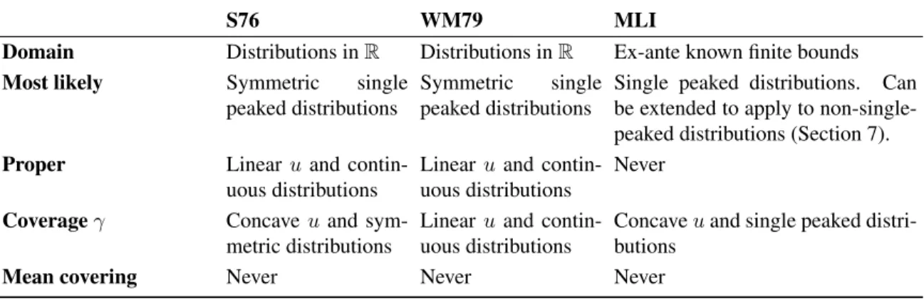
Table 1: Overview of the assumptions underlying the properties of the different interval scoring rules.
S76 WM79 MLI
Domain Distributions inR Distributions inR Ex-ante known finite bounds
Most likely Symmetric single
peaked distributions
Symmetric single peaked distributions
Single peaked distributions. Can be extended to apply to non-single-peaked distributions (Section 7).
Proper Linearuand
contin-uous distributions
Linearuand contin-uous distributions
Never
Coverageγ Concaveuand
sym-metric distributions
Linearuand contin-uous distributions
Concaveuand single peaked distri-butions
Mean covering Never Never Never
Figure 5: Optimal intervals for MLI, S67, and WM79 when f(x) = 2√1
x,γ= 0.5.
0.0 0.2 0.4 0.6 0.8 1.0
1
2
3
4
5
f(x)
MLI
S76 WM79
Table 1 summarizes the properties of the different scoring rules.
7
Extensions
In this section we discuss some of the assumptions that we have made on the elicitation environment, and propose some extensions of our rule.
7.1
Finite outcome spaces
In many applications the outcome x belongs to a finite set. To capture this, assume that x belongs to X = {a+δ, a+ 2δ, .., a+nδ=b}whereδ >0is the distance between any two points in the grid. In such cases we still
propose to use MLI. It turns out that all properties continue to hold, except one can no longer guarantee coverageγbut only coverageγ−ε, whereεis a decreasing function ofδ.
7.2
Multi-peaked distributions and MLMI
Sometimes beliefs may reasonably be expected to have more than one peak. Our method can be adapted to allow for this possibility. Give the expert the opportunity to submit multi-ple nonintersecting intervals. Pay the expert when the event lies in one of the intervals the amount specified bySMgiven
in (1) except thatW now is equal to the sum of the widths of all intervals reported by the expert. We call the resulting rule the Most Likely Multiple Interval elicitation rule, short MLMI. All results carry over to this setting. The only dif-ference is that now beliefs can distributed according to any continuous distribution.
7.3
Eliciting tail risk and the OMLI
As we remarked in Section 4, the MLI can also be used to understand tail risks. The idea is to elicit an interval in the domain of losses, where one fixes the lower bound of the interval at a loss of 0. The expert thus only chooses the upper boundU, but payments are otherwise the same as for the MLI, resulting in the One-sided Most Likely Interval elicitation rule (OMLI).
the valueU then constitutes an upper bound on thep-VaR as believed by the expert.
7.4
Improved precision and the TMLI
Another criterion to select amongst interval scoring rules is to pick the one that pins down the massγwith most preci-sion. To get maximum precision, one would like to pick the rule that implements the smallest width of the expert’s op-timal interval for given coverageγ, beliefs FX and
prefer-encesu. The question is how one should aggregate over all possible beliefs and preferences. Casella and Hwang (1991) propose to measure precision in terms of the ‘worst case’ belief distribution that induces the maximal interval width, and select the rule that minimizes this maximal width.
Definition 4 (Minmax width). S with coverage γ attains
“minmax width withinS” if there is no scoring ruleS˜∈ S
with coverageγsuch that
sup FX∈∆,u∈U
wFX,S, u˜
< sup FX∈∆,u∈U
w(FX, S, u).
The problem with the scoring rules discussed above is that when the expert is very risk averse, she will specify inter-vals that are larger than necessary to coverγ. In order to counter this tendency, one can specify a maximum width of the interval for which the expert can earn positive payoffs. The resulting Truncated Most Likely Interval elicitation rule (TMLI) is given by
SM(L, U, x) =
1− W b−a
g
ifx∈[L, U]
andW ≤γ(b−a)
0 otherwise.
Thus, there is no payment if the expert specifies an inter-val larger than a fraction γ of the range[a, b]. The ratio-nale is that for the worst-case uniform distribution, this frac-tion covers exactlyγ, while for other single-peaked belief distributions one can cover γ in a smaller interval. Thus, the TMLI punishes the expert for specifying a range that is larger than necessary to obtain coverage, and in fact obtains minmax width amongst all interval scoring rules with cov-erageγ.11
8
Conclusion
Eliciting belief intervals is a good way to gain a quick and intuitive understanding of both the events that the expert
11The proof of this claim is simple: In order to cover massγunder the
worst case uniform distribution one needs to have an interval width of at leastγ(b−a). Hence the maximal width of any rule is at least this number. The TMLI, by its definition, never elicits a larger interval, and hence attains minmax width.
thinks likely to occur and the dispersion of an expert’s be-liefs. The Most Likely Interval elicitation rule’ is easily im-plementable, performs well in economic experiments and satisfies a number of desirable theoretical properties. On the basis of these qualities, we believe the MLI can be a valuable tool for practitioners and experimentalists.
The appeal of confidence intervals merits further work into interval scoring rules. On the empirical side, it will be necessary to compare the performance of these and other in-terval scoring rules. On the theoretical side, there are further questions about the trade-offs in designing interval scoring rules, for example between the complexity of the rule and its desired theoretical properties (Schlag & Van der Weele, 2014). The aggregation of different intervals is also an im-portant research area. While the results reported in Section 3 and in Peeters and Wolk (2014) indicate that aggregated in-tervals are reasonably well-calibrated, the theoretical prop-erties of these aggregates are not yet understood.
Another interesting topic is how to combine incentives for truthful reporting with ex-post rewards for well-calibrated forecasts. A naïve approach would be to collect a number of realizations from the random process under considera-tion and then use the MLI or one of the other interval scor-ing rules to compare and score forecasts from several ex-perts.12 However, such rewards may destroy incentives for
truth telling. For instance it is not clear how scoring on the basis of multiple realizations changes the the incentives, as experts may hedge their bets between different elicitations. Another problem is that competition between experts may induce them to become risk seeking, and specify smaller in-tervals or even unlikely events.
References
Aitchison, J., & Dunsmore, I. (1968). Linear-loss interval estimation of location and scale parameters. Biometrika, 55(1), 141–148.
Armantier, O., & Treich, N. (2013). Eliciting beliefs: Proper scoring rules, incentives, stakes and hedging. European Economic Review, 62, 17–40.
Blavatskyy, P. R. (2008). Betting on own knowledge: Ex-perimental test of overconfidence. Journal of Risk and Uncertainty, 38(1), 39–49.
Budescu, D. V., & Du, N. (2007). Coherence and consis-tency of investors? Probability Judgments. Management Science, 53(11), 1731–1744.
Casella, G., & Hwang, J. (1991). Evaluating confidence sets using loss functions.Statistica Sinica, 1, 159–173. Cesarini, D., Sandewall, O., & Johannesson, M. (2006).
Confidence interval estimation tasks and the economics
12In the spirit in which we designed the MLI, one would first determine
of overconfidence. Journal of Economic Behavior & Or-ganization, 61(3), 453–470.
Cettolin, E., & Riedl, A. (2013). Justice under Uncertainty. SSRN Electronic Journal.
Cettolin, E., & Riedl, A. (2015). Partial coercion, con-ditional cooperation, and self-commitment in voluntary contributions to public goods. In S. Winer & J. Martinez (Eds.), Coercion and Social Welfare in Public Finance: Economic and Political Dimensions, Cambridge Univer-sity Press.
Galbiati, R., Schlag, K. H., & Van der Weele, J. J. (2013). Sanctions that signal: An experiment. Journal of Eco-nomic Behavior & Organization, 94, 34–51.
Gneiting, T., & Raftery, A. E. (2007). Strictly Proper Scor-ing Rules, Prediction, and Estimation. Journal of the American Statistical Association, 102(477), 359–378. Hamill, T., & Wilks, D. (1995). A Probabilistic
Fore-cast Contest and the Difficulty in Assesssing Short-Range Forecast Uncertainty.Weather and Forecasting, 10. Harrison, G. W., Martínez-Correa, J., Swarthout, J. T., &
Ulm, E. R. (2013a). Scoring Rules for Subjective Prob-ability Distributions. Manuscript, Georgia State Univer-sity.
Harrison, G. W., Martínez-Correa, J.,& Swarthout, J. T. (2013b). Inducing Risk Neutral Preferences with Binary Lotteries: A Reconsideration. Journal of Economic Be-havior & Organization, 94, 145?159.
Holt, C. A., & Laury, S. (2002). Risk Aversion and Incentive Effects.The American Economic Review, 92(5), 1644. Hossain, T., & Okui, R. (2013). The Binarized Scoring
Rule.The Review of Economic Studies, 80(3), 984–1001. Krawczyk, M. (2011). Overconfident for real? Proper scor-ing for confidence intervals. Manuscript, University of Warsaw.
Mahieu, P.-A., Wolff, F.-C., & Shogren, J. (2014). Inter-val Bidding in a Distribution Elicitation Format. FAERE Working Paper, 16.
Matheson, J., & Winkler, R. (1976). Scoring rules for con-tinuous probability distributions. Management Science, 22(10), 1087–1096.
Moore, D. A., & Healy, P. J. (2008). The trouble with over-confidence.Psychological review, 115(2), 502–517. Murphy, A., & Winkler, R. (1974). Credible interval
tem-perature forecasting: some experimental results.Monthly Weather Review, 102, 784–794.
Offerman, T., Sonnemans, J., Van de Kuilen, G., & Wakker, P. P. (2009). A truth serum for non-bayesians. Review of Economic Studies, 76(4), 1461–1489.
Peeters, R., Vorsatz, M., & Walzl, M. (2015). Beliefs and truth-telling: A laboratory experiment. Journal of Eco-nomic Behavior & Organization, 113, 1–12.
Peeters, R., and Wolk, L. (2014). Eliciting and aggregating individ- ual expectations: An experimental study. Maas-tricht RM Working Paper, 14/029.
Russo, J., & Schoemaker, P. (1992). Managing Overconfi-dence.Sloan Management Review, 33(2), 7–17.
Schlag, K. H., Tremewan, J., & Van der Weele, J. J. (2015). A penny for your thoughts: A survey of methods for elic-iting beliefs.Experimental Economics, 18(3), 457–490. Schlag, K. H., & Van der Weele, J. J. (2013). Eliciting
probabilities, means, medians, variances and covariances without assuming risk neutrality. Theoretical Economics Letters, 3(1), 38–42.
Schlag, K. H., & Van der Weele, J. J. (2014). Eliciting be-liefs with intervals. SSRN Working Paper.
Schmalensee, R. (1976). An experimental study of expecta-tion formaexpecta-tion.Econometrica, 44(1), 17–41.
Selten, R., Sadrieh, A., & Abbink, K. (1999). Money does not induce risk neutral behavior, but binary lotteries do even worse.Theory and Decision, 46, 211–249.
Tausch, F., Potters, J., & Riedl, A. (2014). An experimen-tal investigation of risk sharing and adverse selec- tion. Journal of Risk and Uncertainty, 48(2), 167–186. Winkler, R. (1972). A decision-theoretic approach to
inter-val estimation. Journal of the American Statistical Asso-ciation, 67(337), 187–191.
Winkler, R., & Murphy, A. (1979). The use of probabili-ties in forecasts of maximum and minimum temperatures. The Meteorological Magazine, 108(1288), 317–329. Yaniv, I., & Foster, D. (1997). Precision and accuracy of
judgmental estimation. Journal of Behavioral Decision Making, 10, 21–32.
Appendix with proofs
We assume throughout thatu(0) = 0,a = 0andb = 1. Note that this can be done without loss of generality by appropriate rescaling of the scoring rule. If S is a scor-ing rule for X ∈ ∆ [0,1] with coverage γ then S¯ is a scoring rule for X ∈ ∆ [a, b] with the same coverage if
¯
S(L, U, x) =SL−a b−a,
U−a b−a,
x−a b−a
.
Proof of Proposition 1. By an extension of the extreme value theorem, we know that an upper semi-continuous function attains a maximum on a compact domain. Hence, the proof is complete once we show that u(SM(L, U, X)) is upper semi-continuous in L and U.
Note that u(1−(U−L)) 1−γ
γ
is continuous in L and U. So all we have to show is thatPr (X∈[L, U]) is up-per semi-continuous, i.e. for every L0, U0 with L0 ≤
U0 and every ε > 0 we need to show that there
ex-ists δ > 0 such that k(L, U)−(L0, U0)k < δ
im-plies Pr (X ∈[L, U]) ≤ Pr (X ∈[L0, U0]) + ε. Since Pr (X ∈[L, U]) ≤Pr (X∈[min{L, L0},max{U, U0}])
it is sufficient to prove the claim for [L, U] such that
Note thatPr (X ∈[L, U]) = Pr (X≤U)−Pr (X < L). Note that the cdf FX of X is right-continuous and
non-decreasing. This implies that Pr (X ≤U) = F(U) is right continuous in U. Thus, for everyε > 0there exists δ > 0 such thatU ≤ U0+δimplies thatPr (X ≤U) ≤ Pr (X≤U0) +ε/2. Let FX−(x) = P(X < x), which
is left-continuous and non-increasing. This implies that
Pr (X < L) = FX−(L)is left continuous inL. Again, for everyε >0there existsδ >0such thatL≥L0−δimplies
thatPr (X < L)≥Pr (X < L0)−ε/2.
This implies Pr (X ∈[L, U]) ≤ Pr (X∈[L0, U0]) +
ε, which means that u(SM(L, U, X)) is upper
semi-continuous.
Proof of Proposition 4. The outline of the proof is as fol-lows. In step 1 we derive some properties of the distri-bution function of X. In step2 we separate the problem into the one of finding the best choice ofLandU for given W =wand the problem of how to find the bestw.In step
3we show that expected utility is increasing inwwhenever M(w)< γ.
Step 1. SinceFX is monotonically increasing, it is
dif-ferentiable almost everywhere (see, e.g., Gordon 1994, p. 514).13 Letf be its derivative when it exists and right
con-tinuous otherwise. So f ≥ 0. Since X is single-peaked, there existsx0 such thatf is monotonically increasing for
x < x0and monotonically decreasing forx > x0and any
mass point ofX must be equal tox0.In particular,X has
at most one mass point. Letξ = Pr (X=x0).Together,
this implies thatFX(x) =R0xf(x)dx+ξ∗1{x≥x0}. Since
f is monotone on either side ofx0, it follows thatf is
dif-ferentiable almost everywhere, in particularfis continuous almost everywhere.
Step 2. For each w ∈ [0, γ] let
h(w) = (1−w) 1−γ
γ and let M(w) =
P(X ∈[L∗(w), U∗(w)]) where (L∗(w), U∗(w)) ∈ arg maxL,U:U−L=Wu(SM(L, U, X)). Thus M is
in-creasing inw,hence differentiable almost everywhere. Step 3.Considerw∈[0, γ]such thatM is differentiable atw.Thend(u(h(wdw))M(w))is equal to
M′(w)u(h(w)) +M(w)u′(h(w))h′(w) =M′(w)u(h(w))−
M(w)u′(h(w))
1−γ γ
h(w) 1−w
. (3)
13‘Almost everywhere’ means that the set of points whereF
X is not
differentiable has Lebesgue measure0.
Asu′is concave,u′(z)≤u(z)/zand hence
d(u(h(w))M(w)))
dw ≥
M′(w)u(h(w))−M(w)u′(h(w)) 1−γ
γ
h(w) 1−w
.
(4)
Note thatM is concave by single-peakedness ofX.Hence, the incremental massM′(w)captured by increasingw is
decreasing, so the mass1−M(w)not covered is at most equal to the marginal increase in mass M′(w)due to
en-largeningwtimes the part of the parameter space not cov-ered1−w.In other words,1−M(w)≤M′(w) (1−w).
Substituting this in (4) and rearranging terms yields
d(u(h(w))M(w))
dw ≥
1−M(w)
γ
u(h(w))
1−w .
Hence we have shown that ifwis such thatM′(w)exists
andM(w)< γthendudw(·)>0. Therefore,M∗≥γ.
Proof of Proposition 5. Consider random variables X, Y andXεas in Definition 3. Let[L∗ε, Uε∗]be the optimal
inter-val selected underXεand letWε∗=Uε∗−L∗ε.LetMε(w) =
P(Xε∈[L∗(w), U∗(w)])soMε(w) = (1−ε)M0(w)+
εw. Assume that d
dw(u(h)M0) ≥ 0. AsM0 is concave
in w, M′
0 ≤ M0/w, it follows that dwd (u(h)M0) =
u′(h)h′M0 + u(h)M′
0 ≤ u′(h)h′+w1u(h)
M0.
Hence, d
dw(u(h)Mε) = (1−ε) d
dw(u(h)M0) +
ε u′(h)h′+ 1 wu(h)
w ≥0.Asγ ≥ 1/2, SM is
single-peaked and henceW∗ ε ≥W0∗.
Proof of Proposition 6. Again we use the first order condi-tions which, givenγ ≥ 1/2,are sufficient. Consider con-cave functionsu,uˆandgsuch thatuˆ(x) =g(u(x)). Using concavity ofgwe obtain
d(u(h(w))M(w))
dw =g
′(u(h))u′(h)h′M + ˆuM′
≥
1
u(h)u
′(h)h′M +M′
g(u(h)).
So if
d(u(h(w))M(w))
dw =u
′(h)h′M +u(h)M′ ≥0