Dissolved oxygen prediction using a possibility-theory based fuzzy neural network

(1)

HESSD

12, 12311–12376, 2015

Dissolved oxygen prediction using a possibility-theory based fuzzy neural

network

U. T. Khan and C. Valeo

Title Page

Abstract Introduction

Conclusions References

Tables Figures

◭ ◮

Back Close

Full Screen / Esc

Printer-friendly Version

Interactive Discussion

Discussion

P

a

per

|

Discussion

P

a

per

|

Discussion

P

a

per

|

Discussion

P

a

per

|

Hydrol. Earth Syst. Sci. Discuss., 12, 12311–12376, 2015 www.hydrol-earth-syst-sci-discuss.net/12/12311/2015/ doi:10.5194/hessd-12-12311-2015

This discussion paper is/has been under review for the journal Hydrology and Earth System Sciences (HESS). Please refer to the corresponding final paper in HESS if available.

Dissolved oxygen prediction using a

possibility-theory based fuzzy neural

network

U. T. Khan and C. Valeo

Mechanical Engineering, University of Victoria, P.O. Box 1700, Stn. CSC, Victoria, BC, V8W 2Y2, Canada

Received: 16 October 2015 – Accepted: 13 November 2015 – Published: 26 November 2015

Correspondence to: C. Valeo (valeo@uvic.ca)

(2)

HESSD

12, 12311–12376, 2015

network

Title Page

Tables Figures

◭ ◮

Back Close

Full Screen / Esc

Discussion

P

a

per

|

Discussion

P

a

per

|

Discussion

P

a

per

|

Discussion

P

a

per

|

Abstract

A new fuzzy neural network method to predict minimum dissolved oxygen (DO) con-centration in a highly urbanised riverine environment (in Calgary, Canada) is proposed. The method uses abiotic (non-living, physical and chemical attributes) as inputs to the model, since the physical mechanisms governing DO in the river are largely unknown. 5

A new two-step method to construct fuzzy numbers using observations is proposed. Then an existing fuzzy neural network is modified to account for fuzzy number inputs and also uses possibility-theory based intervals to train the network. Results demon-strate that the method is particularly well suited to predict low DO events in the Bow River. Model output and a defuzzification technique is used to estimate the risk of low 10

DO so that water resource managers can implement strategies to prevent the occur-rence of low DO.

1 Introduction

The City of Calgary is a major economic hub in western Canada. With a rapidly growing population, currently estimated in excess of 1 million, the City is undergoing expansion 15

and urbanisation to accommodate the changes. The Bow River is a relatively small river

(with an average annual flow of 90 m3s−1, with an average width of 100 m, and depth

of 1.5 m) that flows through the City and provides approximately 60 % of the residents with potable water (Khan and Valeo, 2015a, b). In addition to this, water is diverted from within the City for irrigation, is used as a source for commercial and recreational 20

fisheries, and is the source of drinking water for communities downstream of Calgary (Robinson et al., 2009; Bow River Basin Council, 2015). This highlights the importance of the Bow River, not just as a source of potable water, but also as a major economic resource.

However, urbanisation has the potential to reduce the health of the Bow River, which 25

(3)

HESSD

12, 12311–12376, 2015

network

Title Page

Tables Figures

◭ ◮

Back Close

Full Screen / Esc

Discussion

P

a

per

|

Discussion

P

a

per

|

Discussion

P

a

per

|

Discussion

P

a

per

|

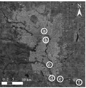
Alberta (Bow River Basin Council, 2015). Three wastewater treatment plants (shown

in Fig. 1) and numerous stormwater outfalls discharge their eﬄ_{uent into the River and}

are considered to be a major cause of water quality degradation in the River (He et al., 2015). This highlights some of the major impacts on the Bow River from the surrounding urban area. A number of municipal and provincial programs are in place to reduce the 5

loading of nutrients and sediments into the river such as the Total Loadings Manage-ment Plan and the Bow River Phosphorus ManageManage-ment Plan (Neupane et al., 2014)

as well as modelling eﬀ_{orts – namely the Bow River Water Quality Model (Tetra Tech,}

2013; Golder, 2004) – to predict the impact of diﬀ_{erent water management programs}

on the water quality. 10

One of the major concerns is that low dissolved oxygen (DO) concentration has oc-curred on a number of occasions over the last decade in the Bow River within the City limits. DO is an indicator of overall health of the aquatic ecosystem (Dorfman and Ja-coby, 1972; Hall, 1984; Canadian Council of Ministers of the Environment, 1999; Kan-nel et al., 2007; Khan and Valeo, 2014a, 2015a), and low DO – which can be caused 15

by a number of diﬀ_{erent factors (Pogue and Anderson, 1995; Hauer and Hill, 2007; He}

et al., 2011; Wen et al., 2013) – can impact various organisms in the waterbody. While

the impact of long-term eﬀ_{ects of low DO are largely unknown, acute events can have}

devastating eﬀ_{ects on aquatic ecosystems (Adams et al., 2013). Thus, maintaining}

a suitably high DO concentration, and water quality in general, is of utmost importance 20

to the City of Calgary and downstream stakeholders, particularly as the City is being challenged to meet its water quality targets (Robinson et al., 2009).

A number of recent studies have examined the DO in the Bow River, and the factors that impact its concentration. Iwanyshyn et al. (2008) found the diurnal variation in DO and nutrient (nitrate and phosphate) concentration was highly correlated, suggesting 25

(4)

stud-HESSD

12, 12311–12376, 2015

network

Title Page

Tables Figures

◭ ◮

Back Close

Full Screen / Esc

Discussion

P

a

per

|

Discussion

P

a

per

|

Discussion

P

a

per

|

Discussion

P

a

per

|

ies, the seasonality of DO, nutrients, and biological concentration, and external factors (e.g. flood events) were demonstrative of the complexity in understanding river pro-cesses in an urban area, and that consideration of various inputs, outputs and their interaction if important to fully understand the system. He et al. (2011) found that sea-sonal variations in DO in the Bow River could be explained by a combination of abiotic 5

factors (such as climatic and hydrometric conditions), as well as biotic factors. The study found that while photosynthesis and respiration of biota are the main drivers of DO fluctuation, the role of nutrients (from both point and non-point sources) was ambiguous. Neupane et al. (2014) found that organic materials and nutrients from point and non-point sources influence DO concentration in the River. The likelihood 10

of low DO was highest downstream of wastewater treatment plants, and that non-point sources have a significant impact in the open-water season. Using a physically-based model, Neupane et al. (2014) predicted low DO concentration more frequently in the future in the Bow River owing to higher phosphorus concentration in the water, as well as impacts of climate change.

15

A major issue of modelling DO in the Bow River is that rapid urbanisation within the watershed has resulted in substantial changes to land-use characteristics, sediment and nutrient loads, and to other factors that govern DO. Major flood events (like those in 2005 and 2013) completely alter the aquatic ecosystem, while new wastewater treat-ment plants (e.g. the Pine Creek wastewater treattreat-ment plant) added in response to the 20

growing population further increases the stress downstream. These types of changes in a watershed increase the complexity of the system, making DO trends and variability more challenging to model. The interaction of numerous factors, over a relatively small

area and across diﬀ_{erent temporal scales means that DO trends in urban areas are}

more diﬃ_{cult to predict and evaluating water quality in urban riverine environments is}

25

a diﬃ_{cult task (Hall, 1984; Niemczynowicz, 1999).}

(5)

under-HESSD

12, 12311–12376, 2015

network

Title Page

Tables Figures

◭ ◮

Back Close

Full Screen / Esc

Discussion

P

a

per

|

Discussion

P

a

per

|

Discussion

P

a

per

|

Discussion

P

a

per

|

stood, in a rapidly changing urban environment. Physically-based models require the

parameterisation of a several diﬀ_{erent variables which may be unavailable, expensive}

and time consuming (Antanasijević_{et al., 2014; Wen et al., 2013; Khan et al., 2013). In}

addition to this, the increase in complexity in an urban system proportionally increases the uncertainty in the system. This uncertainty can arise as a result of vaguely known 5

relationships among all the factors that influence DO, in addition to the inherent ran-domness in the system (Deng et al., 2011). The rapid changes in an urban area render

the systemdynamic as opposed tostationary, which is what is typically assumed for

many probability-based uncertainty quantification methods. Thus, not only is DO

pre-diction diﬃ_{cult, it is beset with uncertainty, hindering water resource managers from}

10

making objective decisions.

In this research, we propose a new method to predict DO concentration in the Bow River using a data-driven approach, as opposed to a physically-based method, that

usespossibilitytheory and fuzzy numbers to represent the uncertainty rather than the

more commonly used probability theory. Data-driven models are a class of numer-15

ical models based on generalised relationships, links or connections between input and output datasets (Solomantine and Ostfeld, 2008). These models can characterize a system with limited assumptions and are useful in solving practical problems, espe-cially when there is lack of understanding of the underlying physical process, the time

series are of insuﬃ_{cient length, or when existing models are inadequate (Solomatine}

20

et al., 2008; Napolitano et al., 2011).

1.1 Fuzzy numbers and data-driven modelling

Possibility theory is an information theory that is an extension of fuzzy sets theory for

representing uncertain, vague or imprecise information (Zadeh, 1978). Fuzzynumbers

are an extension of fuzzy set theory, and express an uncertain or imprecisequantity.

25

(6)

HESSD

12, 12311–12376, 2015

network

Title Page

Tables Figures

◭ ◮

Back Close

Full Screen / Esc

Discussion

P

a

per

|

Discussion

P

a

per

|

Discussion

P

a

per

|

Discussion

P

a

per

|

exists. This type of uncertainty is in contrast to aleatory uncertainty that is typically handled using probability theory. Possibility theory and fuzzy numbers are thus useful when a probabilistic representation of parameters may not be possible, since the exact values of parameters may be unknown, or only partial information is available (Zhang, 2009). Thus, the choice of using a data-driven approach in combination with possibility 5

theory lends itself well to the constraints posed by the problem in the Bow River: the

diﬃ_{culty in correctly defining a physically-based model for a complex urban system and}

the use of possibility theory to model the uncertainty in the system when probability theory based methods may be inadequate.

Data-driven models, such as neural networks, regression-based techniques, fuzzy 10

rule–based systems, and genetic programming, have seen widespread use in hydrol-ogy, including DO prediction in rivers (Shrestha and Solomatine, 2008; Solomatine et al., 2008; Elshorbagy et al., 2010). Wen et al. (2011) used artificial neural networks (ANN) to predict DO in a river in China using ion concentration as the predictors.

An-tanasijević _{et al. (2014) used ANNs to predict DO in a river in Serbia using a Monte}

15

Carlo approach to quantify the uncertainty in model predictions and temperature as a predictor. Chang et al. (2015) also used ANNs coupled with hydrological factors (such as precipitation and discharge) to predict DO in a river in Taiwan. Singh et al. (2009) used water quality parameters to predict DO and BOD in a river in India. Other stud-ies (e.g. Heddam, 2014; Ay and Kisi, 2012) have used regression to predict DO in 20

rivers using water temperature, or electrical conductivity, amongst others, as inputs. In general, these studies have demonstrated that there is a need and demand for less complex DO models, has led to an increase in the popularity of data-driven models

(An-tanasijević_{et al., 2014), and that the performance of these models is suitable. Recent}

research into predicting DO concentration in the Bow River in Calgary using abiotic 25

(7)

HESSD

12, 12311–12376, 2015

network

Title Page

Tables Figures

◭ ◮

Back Close

Full Screen / Esc

Discussion

P

a

per

|

Discussion

P

a

per

|

Discussion

P

a

per

|

Discussion

P

a

per

|

the factors (e.g. increasing the discharge rate downstream of a treatment plant) can potentially reduce the risk of low DO.

While fuzzy set theory based applications, particularly applications using fuzzylogic

in neural networks, have been widely used in many fields including hydrology

(Bár-dossy et al., 2006; Abrahart et al., 2010), the use of fuzzynumbersand possibility

the-5

ory based applications has been limited in comparison (Bárdossy et al., 2006; Jacquin, 2010). Some examples include maps of soil hydrological properties (Martin-Clouaire et al., 2000), remotely sensed soil moisture data (Verhoest et al., 2007), climate mod-elling (Mujumdar and Ghosh, 2008), subsurface contaminant transport (Zhang et al., 2009), and streamflow forecasting (Alvisi and Franchini, 2011). Khan et al. (2013) and 10

Khan and Valeo (2015a) have introduced a fuzzy number basedregressiontechnique

to model daily DO in the Bow River using abiotic factors with promising results. Sim-ilarly, Khan and Valeo (2014a) used an autoregressive time series based approach combined with fuzzy numbers to predict DO in the Bow River. In these studies the use of fuzzy numbers meant that the uncertainty in the system could be quantified 15

and propagated through the model. However, due to the highly non-linear nature of DO modelling, the use of an ANN based method is of interest since these types of

models are eﬀ_{ective for modelling complex, nonlinear relationships without the explicit}

understanding of the physical phenomenon governing the system. A fuzzy neural net-work method proposed by Alvisi and Franchini (2011) for streamflow prediction that 20

uses fuzzy weights and biases in the network, is further refined in this research for predicting DO concentration.

1.2 Objectives

Given the importance of DO concentration as an indicator of overall aquatic ecosys-tem health, there is a need to accurately model and predict DO in urban riverine en-25

(8)

Fran-HESSD

12, 12311–12376, 2015

network

Title Page

Tables Figures

◭ ◮

Back Close

Full Screen / Esc

Discussion

P

a

per

|

Discussion

P

a

per

|

Discussion

P

a

per

|

Discussion

P

a

per

|

chini (2011) is adapted and extended in two critical ways. The existing method uses crisp (i.e. non-fuzzy) inputs and outputs to train the network, producing a set of fuzzy number weights and biases, and fuzzy outputs. The method is adapted to be able to handle fuzzy number inputs to produce fuzzy weights and biases, and fuzzy outputs. The advantage is that the uncertainties in the input observations are also captured 5

within the model structure. To do this, a new method of creating fuzzy numbers from observations is presented based on a probability-possibility transformation. Second, the existing training algorithm is based on capturing a predetermined set of observa-tions (e.g. 100, 95 or 90 %) within the fuzzy outputs. The selection of the predetermined set of observations in the original study was an arbitrary selection. A new method that 10

exploits the relationship between possibility theory and probability theory is defined to create a more objective method of training the FNN. A consequence of this is that the resulting fuzzy number outputs from the model can then be directly used for risk analysis, specifically to quantify the risk of low DO concentration. This information is extremely valuable for managing water resources in the face of uncertainty.

15

Following previous research for this river, two abiotic inputs (daily mean water

tem-perature, T and daily mean flow rate, Q) will be used to predict daily minimum DO.

An advantage of using these factors is that they are routinely collected by the City of Calgary, and thus, a large dataset is available. Also, their use in previous studies has shown that they are good predictors of daily DO concentration in this river basin (He 20

et al., 2011; Khan et al., 2013; Khan and Valeo, 2015a). The following sections outline the background of fuzzy numbers and existing probability-possibility transformations. This is followed by the development of the new method to create fuzzy numbers from observations. Then, the new FNN method using fuzzy inputs is developed mathemat-ically using new criteria for training, also based on possibility theory. Lastly, a method 25

(9)

HESSD

12, 12311–12376, 2015

network

Title Page

Tables Figures

◭ ◮

Back Close

Full Screen / Esc

Discussion

P

a

per

|

Discussion

P

a

per

|

Discussion

P

a

per

|

Discussion

P

a

per

|

2 Methods

2.1 Data collection

The Bow River is 645 km long and averages a 0.4 % slope over its length (Bow River Basin Council, 2015) from its headwaters at Bow Lake in the Rocky Mountains to its confluence with the Oldman River in Southern Alberta, Canada (Robinson et al., 2009; 5

Environment Canada, 2015). The river is supplied by snowmelt from the Rocky Moun-tains, rainfall and discharge from groundwater. The City of Calgary is located within the

Bow River Basin and the river has an average annual discharge of 90 m3s−1, an

aver-age width and depth of 100 and 1.5 m, respectively (Khan and Valeo, 2014b, 2015b). The City of Calgary routinely samples a variety of water quality parameters along 10

the Bow River to measure the impacts of urbanisation, particularly from three

wastew-ater treatment plants and numerous stormwwastew-ater runoﬀ_{outfalls that discharge into the}

River. DO concentration measured upstream of the City is generally high throughout the year, with little diurnal variation (He et al., 2011; Khan et al., 2013; Khan and Valeo, 2015a). The DO concentration downstream of the City is lower and experiences much 15

higher diurnal fluctuation. The three wastewater treatment plants are located upstream of this monitoring site, and are thought to be responsible, along with other impacts of urbanisation, for the degradation of water quality (He et al., 2015).

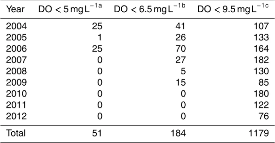
For this research, nine years of DO concentration data was collected from one of the downstream stations from 2004 to 2012. The monitoring station was located at 20

Pine Creek and sampled water quality data every 30 min (from 2004 to 2005), and every 15 min (from 2006 to 2007). The station was then moved to Stier’s Ranch and sampled data every hour (in 2008) and every 15 min (2009 to 2011). The monitoring site was moved further downstream to its current location (at Highwood) in 2012 where it samples every 15 min. During this period a number of low DO events have been 25

observed in the River and are summarised below in Table 1 corresponding to diﬀ_erent

(10)

HESSD

12, 12311–12376, 2015

network

Title Page

Tables Figures

◭ ◮

Back Close

Full Screen / Esc

Discussion

P

a

per

|

Discussion

P

a

per

|

Discussion

P

a

per

|

Discussion

P

a

per

|

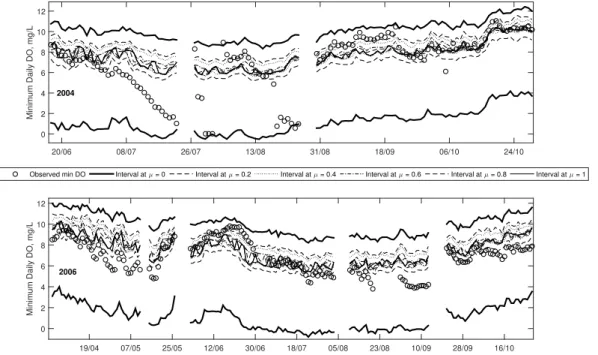
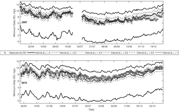
Note that even though daily minimum DO was observed to be below 5 mg L−1on

sev-eral occasions in 2004 and 2006 (in Table 1), the minimum DO was below 9.5 mg L−1

only 107 and 164 days, respectively, for those two years. In contrast, in 2007 and 2010,

no observations below 5 mg L−1 are seen yet 182 and 180 days, respectively, below

the 9.5 mg L−1 guideline were seen for those years. The total amount of days below

5

9.5 mg L−1constitute approximately 90 % of all observations for those years. This

high-lights that despite no DO events below 5 mg L−1, generally speaking minimum DO on

a daily basis was quite low in these two years. The implication of this is that only using one guideline for DO might not be a good indicator of overall aquatic ecosystem health.

A YSI sonde is used to monitor DO andT, and the sonde is not accurate in freezing

10

water, thus only data from the ice free period was considered, which is approximately from April to October for most years (YSI Inc., 2015). Since low DO events usually occur in the summer (corresponding to high water temperature and lower discharge), the ice-free period dataset contains the dates that are of interest for low DO modelling.

Daily mean flow rate,Q, was collected from the Water Survey of Canada site “Bow

15

River at Calgary” (ID: 05BH004) for the same period. This data is collected hourly throughout the year, thus, data where considerable shift corrections were applied (usu-ally due to ice conditions) were removed from the analysis. The mean annual water

temperature ranged between 9.23 and 13.2◦C, and the annual mean flow rate was

between 75 and 146 m3s−1, for the selected period.

20

2.2 Probability-possibility transformations

Fuzzy sets were proposed by Zadeh (1965) in order to express imprecision in complex systems, and can be described as a generalisation of classical set theory (Khan and

Valeo, 2015a). In classical set theory, an elementx either belongs or does not belong

to a set A. In contrast, using fuzzy set theory, the elementsx have a degree of

mem-25

(11)

HESSD

12, 12311–12376, 2015

network

Title Page

Tables Figures

◭ ◮

Back Close

Full Screen / Esc

Discussion

P

a

per

|

Discussion

P

a

per

|

Discussion

P

a

per

|

Discussion

P

a

per

|

A, andµ=_{1 means that it completely belongs in}_A_{, while a value}_µ=_{0.5 means that it}

is only a partial member ofA.

Fuzzynumbers express uncertain or imprecisequantities, and represent the set of

all possible values that define a quantity rather than a single value. A fuzzy number is

defined as a specific type of fuzzy set: anormalandconvexfuzzy set. Normal implies

5

that there is at least one element in the fuzzy set with a membership level equal to 1, while convex means that the membership function increases monotonically from

the lower support (i.e., µ=₀L_{) to the modal element (i.e. the element(s) with}_µ=₁₎

and then monotonically decreases to the upper support (i.e.,µ=₀R_{) (Kaufmann and}

Gupta, 1985). 10

Traditional representation of a fuzzy numbers has been using symmetrical, linear membership functions, typically denoted as triangular fuzzy numbers. The reason for selecting this type of membership function has to do with its simplicity: given that a fuzzy number must, by definition, be convex and normal, a minimum of three

ele-ments are needed to define a fuzzy number (two eleele-ments atµ=_{0 and one element}

15

at µ=_{1). For example, if the most credible value for DO concentration is 10 mg L}−1

(µ=_{1), with a support about the modal value between (}_µ=₀L_{) and 12 mg L}−1₍_µ=₀R_).

This implies that the simplest membership function is triangular, though not necessar-ily symmetrical. Also, as we demonstrate below, in some probability-possibility frame-works, a triangular membership function corresponds to a uniform probability distribu-20

tion – the least specific distribution in that any value is equally probable and hence, represents the most uncertainty (Dubois and Prade, 2015; Dubois et al., 2004).

However, recent research (Khan et al., 2013; Khan and Valeo, 2014a, b, 2015a, b) has shown that such a simplistic representation may not be appropriate for hydrological data, which is often skewed, and non-linear. This issue is further highlighted if the 25

probability-possibility framework mentioned above is used: it implies that for a triangular

membership function, the fuzzy number bounded by the support [8 12] mg L−1, has

a uniform probability distribution bounded between 8 and 12 mg L−1with a mean value

(12)

HESSD

12, 12311–12376, 2015

network

Title Page

Tables Figures

◭ ◮

Back Close

Full Screen / Esc

Discussion

P

a

per

|

Discussion

P

a

per

|

Discussion

P

a

per

|

Discussion

P

a

per

|

not diﬃ_{cult to see that this an over-simplification of hydrological data, which often have}

skewed, non-symmetrical distributions. In many cases enough information (i.e. from observations) is available to define the membership function with more specificity, and this information should be used to define the membership function.

Multiple frameworks exist to transform a probability distribution to a possibility distri-5

bution, and vice versa; a comparison of diﬀ_{erent conceptual approaches are provided}

in Klir and Parvais (1992), Oussalah (2000), Jaquin (2010), Mauris (2013) and Dubois and Prade (2015). However, a major issue of implementing fuzzy number based meth-ods in hydrology is that there is no consistent, transparent and objective method to convert observations (e.g. time series data) into fuzzy numbers, or generally speak-10

ing to construct the membership function associated with fuzzy values (Abrahart et al., 2010; Dubois and Prade, 1993; Civanlar and Trussel, 1986).

A popular method (Dubois et al., 1993, 2004) converts a probability distribution to a possibility distribution by relating the area under a probability density function to the membership level (Zhang, 2009). From this point of view, the possibility is viewed as 15

the upper envelope of the family of probability measures (Jacquin, 2010; Ferrero et al., 2013; Betrie et al., 2014). There are two important considerations for this transforma-tion, first it guarantees that something must be possible before it is probable; hence, the degree of possibility cannot be less than the degree or probability – this is known as the consistency principle (Zadeh, 1965). Second is order preservation, which means if 20

the possibility ofx_i is greater than the possibility ofx_j then the probability ofx_i must be

greater than the probability ofx_j (Dubois et al., 2004). For a discrete system, this can

be represented as:

ifp(x1)> p(x2)> . . . > p(xn),

then the possibility distribution ofx (π(x)), follows the same order, that is: 25

π(x1)> π(x2)> . . . > π(xn).

(13)

HESSD

12, 12311–12376, 2015

network

Title Page

Tables Figures

◭ ◮

Back Close

Full Screen / Esc

Discussion

P

a

per

|

Discussion

P

a

per

|

Discussion

P

a

per

|

Discussion

P

a

per

|

Forp(x1)> p(x2)> . . . > p(xn):

π(x1)=1

f(x)=

(Pn

j=ipj, ifpi−1> pi

π(xi−1), else

(1)

where the x_i are elements of a fuzzy number A, π(x_i) is the possibility of element

xi, and p(xi) is the probability of elementxi. The concept of this transformation may

5

be more illustrative when viewed in the continuous case: for any interval [a,b], the

membership levelµ(whereπ(a)=_π₍_b₎=_µ_{) is equal to the sum of the areas under the}

probability density function curve between (−∞,a) and (b,∞) (Zhang et al., 2009). It is

important to highlight that this particular transformation has an inverse transformation associated with, where a probability distribution can be estimated from the possibility 10

distribution.

However, a major drawback of this transformation is that it theoretically requires a full description of the probability density function, or in the finite case, the probability asso-ciated with each element of the fuzzy number, the probability mass function. For many hydrology and time series based applications this might not be possible because the 15

hourly data (that is typically collected) may not adequately fit the mould of a known class of probability density functions, or one distribution amongst many alternatives may have to be selected based on best-fit. This best-fit function may not be univer-sal, e.g. data from one 24 h period may be best described by one class or family of

probability density function, while the next day by a completely diﬀ_{erent class of}

den-20

sity function. This means working with multiple classes of distribution functions for one application, which can be cumbersome. Also, given that each day may only have 24

data points (or fewer on days with missed samples) it is diﬃ_{cult to select one particular}

function.

In previous research by Khan and Valeo (2015a), a new approach to create a fuzzy 25

(14)

HESSD

12, 12311–12376, 2015

network

Title Page

Tables Figures

◭ ◮

Back Close

Full Screen / Esc

Discussion

P

a

per

|

Discussion

P

a

per

|

Discussion

P

a

per

|

Discussion

P

a

per

|

was used to estimate the membership function of the fuzzy number. To create the his-togram, the bin-size was selected based on the extrema observations for a given day and the number of the observations. A linear interpolation scheme was then used to calculate the values of the fuzzy number at five predefined membership levels. This method has a few short-comings, namely: the bin-size selection was arbitrarily selected 5

based on the magnitude and number of observations which does not necessarily result in the optimum bin-size. This lack of optimality means that the resulting histogram may either be too smooth so as not to capture the variability between membership levels, or too rough and uneven so that the underlying shape of the membership function is

diﬃ_{cult to discern. This is a common issue with histogram selection in many}

applica-10

tions (Shimazaki and Shinomoto, 2007). Secondly, the aforementioned transformation

used by Khan and Valeo (2015a) only allows one element to have µ=_{1 when} _p₍_x₎

is maximum. However, there are a number of cases (e.g. bimodal distributions, or ar-rays when all elements are equal) where multiple elements have joint-equal maximum

p(x)), and hence multiple elements withµ=_{1. This means that all elements}_within_the

15

α-cut interval [a b]_µ=1 (wherea and b are the minimum and maximum elements with

µ=_{1) must by definition also have a membership level equal to 1. Thus, a method is}

necessary to be flexible enough to accommodate these types of issues.

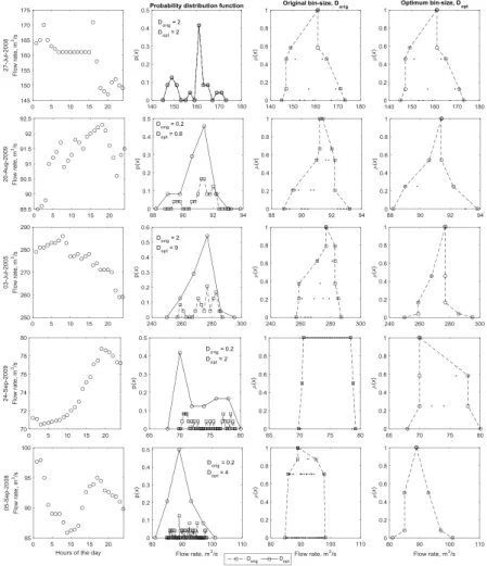
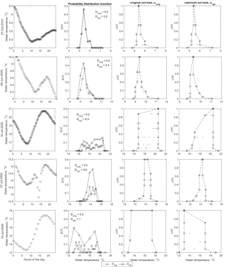
In this research, a two-step procedure is proposed to create fuzzy numbers on the

inputs (i.e.Q and T) using hourly (or sub-hourly) observations. First, a bin-size

opti-20

misation method is used (an extension of an algorithm proposed by Shimazaki and Shinomoto, 2007) to create histograms to represent the estimate of discretised proba-bility density functions of the observations. This estimate of the probaproba-bility distribution is then transformed to the membership function of the fuzzy number using a new nu-merical procedure and the transformation principles described in Eq. (1). This updated 25

method requires no assumptions regarding the distribution of the underlying data or

selection of an arbitrary bin-size, has the flexibility to create diﬀ_{erent shapes of fuzzy}

(15)

el-HESSD

12, 12311–12376, 2015

network

Title Page

Tables Figures

◭ ◮

Back Close

Full Screen / Esc

Discussion

P

a

per

|

Discussion

P

a

per

|

Discussion

P

a

per

|

Discussion

P

a

per

|

ements to have equal µ=_{1. The proposed algorithm is described in the proceeding}

section.

A new algorithm to create fuzzy numbers

Shimazaki and Shinomoto (2007) proposed a method to find the optimum bin-size of a histogram when the underlying distribution of the process is unknown. The basic 5

premise of the method is that the optimum bin-size (Dopt) is one that minimises the

error between the theoretical (but unknown) probability density and the histogram

gen-erated using theDopt. The error metric used by Shimazaki and Shinomoto (2007) is the

mean integrated squared error (E_MISE) which is frequently used for density estimation

problems. It is defined as: 10

EMISE=

1

P

Z

0

E[f_n(t)−f(t)]2dt (2)

wheref(t) is the unknown density function,fn(t) is the histogram estimate of the density

function,t denotes time and P is the observation period, andE[·] is the expectation.

In practice,EMISE cannot be directly calculated since the underlying distribution is

un-known and thus, an estimate of theEMISE is used in its place (see CD below). Thus,

15

f_n(t) can be found without any assumptions of the type of distribution (e.g. class,

uni-modality, etc.); the only assumption is that the number of events (i.e. the countsk_i) in

theith bin of the histogram follow a Poisson point process. This means that the events

in two disjoint bins (e.g. theith and i+_{1th bin) are independent, and that mean (}_k₎

and variance (v) of the k_i in each bin are equal, due to the assumption of a Poisson

20

process (Shimazaki and Shinomoto, 2007).

Using this property, the optimum bin-size can be found as follows. LetXbe the input

data vector for the observation period (P), e.g., a [24×1] vector corresponding to hourly

(16)

HESSD

12, 12311–12376, 2015

network

Title Page

Tables Figures

◭ ◮

Back Close

Full Screen / Esc

Discussion

P

a

per

|

Discussion

P

a

per

|

Discussion

P

a

per

|

Discussion

P

a

per

|

D. The number of events ki in each ith bin are then counted and the mean (k) and

variance (v) of theki are calculated as follows:

k= 1

N

X

i=1

ki (3)

v= 1

N

X

i=1

(k_i−k)2. (4)

Thek andv are then used to compute thecost-functionCD, which is defined as:

5

C_D=2k−v

D2 . (5)

This cost-function is a variant of the originalEMISE listed in Eq. (2) and is derived by

removing the terms fromEMISEthat are independent of the bin-sizeD, and by replacing

the unobservable quantities (i.e.E[f(t)]) with their unbiased estimators (details of this

derivation can be found in the original paper by Shimazaki and Shinomoto, 2007). 10

The objective then is to search forDopt: the value of D that minimisesCD. To do this

two systematic modification are made: first,C_D is recalculated at diﬀ_erent _partitioning

positions, and secondly, the entire process is repeated for diﬀ_{erent values of} _N _and

D, until a “reliable” estimate of minimum CD and thus Dopt is found. Using diﬀerent

partitioning positions means that the variability ink_i resulting from the position of the

15

bin (rather than the size of the bin) can be quantified. Repeating the analysis at diﬀ_erent

N and D accounts for the variability due to diﬀ_{erent bin-sizes. Both these techniques}

are ways of accounting for the uncertainty associated with estimating the histogram. Partitioning positions are defined as the first and last point that define a bin. The most

common way of defining a partitioning position is to centre it on some valuea, e.g. the

20

bin defined at [a−D/2,a+_D/_{2] is centred on} _a _{and has a bin-size} _D_{. Variations of}

(17)

HESSD

12, 12311–12376, 2015

network

Title Page

Tables Figures

◭ ◮

Back Close

Full Screen / Esc

Discussion

P

a

per

|

Discussion

P

a

per

|

Discussion

P

a

per

|

Discussion

P

a

per

|

bin-sizeDis kept constant, but the first and last points are perturbed by a small value

δ: [a−D/2+_δ_,_a+_D/₂+_δ_{], where} _δ _{ranges incrementally between 0 and}_D_{. Using}

these diﬀ_{erent values of}_δ_{whilst keeping}_D_{constant will result in di}ﬀ_{erent values of}_k

i

and hence unique values ofCD. Thus, for a single value ofD, multiple values ofCDare

possible. 5

For this research this bin-size optimisation algorithm is implemented to determine the

optimum histogram for the two input variables,Qand T. The array of daily data,X, (at

hourly or higher frequency, see Sect. 2.1 for details regarding the sampling frequency of both inputs) for each variable was collected for the nine year period. The bin-size was calculated for each day as follows:

10

D=xmax−xmin

N (6)

where thexmaxandxminare the maximum and minimum sampled values forX,

respec-tively, andN is the number of bins. As described above, a number of diﬀ_erent_D _were

considered to find the optimumC_D. This was done by selecting a number of diﬀ_erent

values ofN, ranging from Nmin toNmax. The minimum valueNmin, was set at 3 for all

15

days; this is the necessary number of bins to define a fuzzy number (two elements for

µ=_{0, and one element for}_µ=_{1). The highest value,}_N_max_{was calculated as:}

N=xmax−xmin

2r (7)

where 2r is the measurement resolution of the device used to measure eitherQorT,

set at twice the accuracy (r) of the device. The rational for this decision is that asN

20

increases D necessarily decreases (as per Eq. 6). However, D cannot be less than

the measurement resolution; this constraint (i.e.N≤Nmax) ensures that the optimum

bin-size is never less than what the measurement devices can physically measure. For

this research, the accuracy forT is listed as ±0.1◦C, and thus, the resolution (2r) is

0.2◦C (YSI Inc., 2015). ForQall measurements below 99 m3s−1have an accuracy of

(18)

HESSD

12, 12311–12376, 2015

network

Title Page

Tables Figures

◭ ◮

Back Close

Full Screen / Esc

Discussion

P

a

per

|

Discussion

P

a

per

|

Discussion

P

a

per

|

Discussion

P

a

per

|

±0.1 m3s−1and thus, a resolution of 0.2 m3s−1, while measurements above 99 m3s−1

have an accuracy of ±1 m3s−1, and thus a resolution of 2 m3s−1. This is based on

the fact that all data provided by the Water Survey of Canada is accurate to three

significant figures. Note that for the case wherexmin equals xmax (i.e. no variance in

the daily observed data) thenD=₂_r_{, which means that the only uncertainty considered}

5

is due to the measurement.

Once theNmaxis determined, the bin-sizeDwas calculated for eachNbetweenNmin

andNmax. Then, starting at the largestD(i.e.D=(xmax−xmin)/Nmin), the cost-function

CD is calculated at the firstpartitioning positing, where the first bin is centred atxmin,

[(xmin−D/2)(xmin+D/2)], and the Nth bin is centred on xmax, [(xmax−D/2), (xmax+

10

D/2)]. Then, C_D is calculated at the next partitioning positing, where the first bin is

[(xmin−D/2+δ)(xmin+D/2+δ)], and theNth bin is [(xmax−D/2+δ), (xmax+D/2+δ)].

The value ofδranged between 0 andDat (D/100) intervals. Thus, for this value ofD,

100 values ofC_D were calculated since 100 diﬀ_{erent partitioning positions were used.}

The mean value of these CD was used to define the final cost-function value for the

15

givenD.

This process is then repeated for the next N between Nmin and Nmax, using the

correspondingD at 100 diﬀ_{erent partitioning positions, and so on until the smallest} _D

(atNmax). This results in [Nmax−Nmin] values of meanCD: the value ofDcorresponding

to the minimum value ofC_Dis considered to be the optimum bin-sizeDopt. ThisDoptis

20

then used to construct the optimum histogram of each daily observation. This histogram

can be used to calculate a discretised probability density function (p(x)), where for each

x(an element ofX), thep(x) is calculated by dividing the number of events in each bin

by the total number of elements inX. Thexandp(x) can then be used to calculate the

possibility distribution using the transformation described in Eq. (1). 25

First, the p(x) are ranked from highest to lowest, and the x corresponding to the

highestp(x) is has a membership level of 1. Then the π(x) values for the remaining

x are calculated using Eq. (1). For cases where multiple elements have equal p(x),

the highestπ(x) is assigned to eachx. For example, ifp(x_i)=_p₍_x

(19)

HESSD

12, 12311–12376, 2015

network

Title Page

Tables Figures

◭ ◮

Back Close

Full Screen / Esc

Discussion

P

a

per

|

Discussion

P

a

per

|

Discussion

P

a

per

|

Discussion

P

a

per

|

π(xj)=π(xi). This means that in some cases, for each calculated membership level,

π(x), there exists anα-cut interval [a,b]µ=π(x)where all the elements betweenaandb

have equalp(x) and hence equalπ(x). By definition of α-cut intervals, all values ofx

within the interval [a,b] haveat leasta possibility ofπ(x). A special case of this occurs

when multiplex have joint-equal maximump(x), meaning that multiple elements have

5

a membership level of µ=_{1. Thus, an} _α_{-cut interval is created for the} _µ=_{1 case,}

creating a trapezoidal membership function, where the modal value of the fuzzy number is defined by an interval rather than a single element.

Once all the π(x) are calculated for each element x in X, a discretised empirical

membership function of the fuzzy numberX can be constructed using the calculated

10

α-cut intervals. That is, the fuzzy number is defined by a number of intervals at diﬀ_erent

membership levels. The upper and lower limit of the intervals at higher membership levels define the extent of the limits of the intervals at lower membership levels. This way the constructed fuzzy numbers maintain convexity (similar to a procedure used by Alvisi and Franchini, 2011), where the widest intervals have the lowest membership 15

level. For example, the interval at µ=_{0.2 will contain the interval} _µ=_{0.4, and this}

interval will contain the interval atµ=_0.8.

In creating this discretised empirical membership function this way (rather than as-suming a shape of the function) means that this function best reflects the possibility distribution of the observed data. However, it also means that all fuzzy numbers cre-20

ated using this method are not guaranteed to be defined at the sameπ(x), nor have

an equal number ofπ(x) intervals used to define the fuzzy number. Thus, direct fuzzy

arithmetic between multiple fuzzy numbers using the extension principle is not possible

since it requires each fuzzy number to be defined at the sameα-cut intervals

(Kauf-mann and Gupta, 1985). Thus, linear interpolation is used to define each fuzzy number 25

at a pre-setα-cut interval using the empiricalπ(x) calculated using the transformation.

To select the pre-setα-cut intervals it is illustrative to see the impact of selecting two

extreme cases: (i) if only two levels are selected (specifically µ=_{0 and 1) the}

(20)

HESSD

12, 12311–12376, 2015

network

Title Page

Tables Figures

◭ ◮

Back Close

Full Screen / Esc

Discussion

P

a

per

|

Discussion

P

a

per

|

Discussion

P

a

per

|

Discussion

P

a

per

|

there are important implications of using triangular membership functions that make it undesirable for hydrological data, (ii) if a large number of intervals (e.g. 100 intervals

betweenµ=_{0 and 1) are selected, there is a risk that the number of pre-set intervals}

is much larger than the empiricalπ(x), which means not enough data (empiricalα-cut

levels intervals) to conduct interpolation, leading to equal interpolated values at mul-5

tipleα-cut levels. For this research, results (discussed in the following section) of the

bin-size optimisation showed that most daily observations for T and Q resulted in 2

to 10 uniquep(x) values. Based on this, six pre-set α-cut intervals were selected: 0,

0.2, 0.4, 0.6, 0.8 and 1. The empirical π(x) can then be converted to a standardised

function at pre-defined membership levels using linear interpolation. 10

2.3 Fuzzy neural networks

2.3.1 Background on artificial neural networks

Artificial neural networks (ANN) are a type of data-driven model that are defined as a massively parallel distributed information processing system (Elshorbagy et al., 2010; Wen et al., 2013). As a predictive model, ANNs can capture complex, nonlinear rela-15

tionships that may exist between variables without the explicit understanding of the

physical phenomenon (Alvisi and Franchini, 2011; Antanasijević_{et al., 2014). This has}

resulted in significant use of ANN models in hydrology when the complexity of the phys-ical systems is high owing partially to an incomplete understanding of the underlying process, and the lack of availability of necessary data (He et al., 2011; Kasiviswanathan 20

et al., 2013). Further, ANNs arguably require less data and do not require an

ex-plicit mathematical description of the underlying physical process (Antanasijević_{et al.,}

2014), making it a simpler and practical alternative to traditional modelling techniques. Multilayer Perceptron (MLP) is a type of feedforward ANN and is one of the most commonly used in hydrology (Maier et al., 2010). One of the reasons for the popu-25

(21)

HESSD

12, 12311–12376, 2015

network

Title Page

Tables Figures

◭ ◮

Back Close

Full Screen / Esc

Discussion

P

a

per

|

Discussion

P

a

per

|

Discussion

P

a

per

|

Discussion

P

a

per

|

simple to develop, and theoretically have the capacity of approximating any linear or nonlinear mapping (ASCE 2000; Elshorbagy et al., 2010; Napolitano et al., 2011; Ka-siviswanathan et al., 2013). Further, the popularity of MLP has meant that subsequent research has continued to use MLP (He and Valeo, 2009; Napolitano et al., 2011) and thus, form a reference for the basis of comparing ANN performance (Alvisi and Fran-5

chini, 2011).

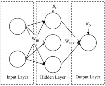
In the simplest case, an MLP consists of an input layer, a hidden layer, and an output layer as shown in Fig. 2. Each layer consists of a number of neurons (or nodes) that each receive a signal, and on the basis of the strength of the signal, emit an output. Thus, the final output layer is the synthesis and transformation of all the input signals 10

from both the input and the hidden layer (He and Valeo, 2009).

The number of neurons in the input (nI) and output (nO) layers corresponds to the

number of variables used as the input and the output, respectively and the number

of neurons in the hidden layer (nH) are selected based on the relative complexity of

the system (Elshorbagy et al., 2010). A typical MLP is expressed mathematically as 15

follows:

y_i=_f

HID(WIHxi+BH) (8)

z_i =_f

OUT(WHOyi+BO) (9)

wherex_i is theith observation (annI×1 vector) from of a total ofnobservations,WIHis

anH×nImatrix of weights between the input and hidden-layer,BHis a vector (nH×1) of

20

biases in the hidden-layer, andy_i is theith output (ann_H×1 vector) of the input signal

through the hidden-layer transfer function,fHID. Similarly,WHOis an nO×nH matrix of

weights between the hidden and output-layers,B_O is annO×1 vector of biases in the

output-layer, andf_OUT the final transfer function to generate theith modelled outputz_i

(annO×1 vector).

25

The values of all the weights and biases in the MLP are calculated by training the

network by minimising the error – typically mean squared error (EMSE) (He and Valeo,

(22)

num-HESSD

12, 12311–12376, 2015

network

Title Page

Tables Figures

◭ ◮

Back Close

Full Screen / Esc

Discussion

P

a

per

|

Discussion

P

a

per

|

Discussion

P

a

per

|

Discussion

P

a

per

|

ber of training algorithms can be used, and one of the most common methods is the Levenberg–Marquardt algorithm (LMA) (Alvisi et al., 2006). In this method, the error between the output and target is back-propagated through the model using a gradient method where the weights and biases are adjusted in the direction of maximum error reduction. The LMA is well-suited for ANN problems that have a relatively small number 5

of neurons. To counteract potential over-fitting issues, an early-stopping procedure is used (Alvisi et al., 2006; Maier et al., 2010), which is a form of regularisation where the data is split into three subsets (for training, validation and testing) and the train-ing is terminated when the error on the validation subset increases from the previous iteration. Most ANNs have a deterministic structure without a quantification of the un-10

certainty corresponding to the predictions (Alvisi and Franchini, 2012; Kasiviswanathan and Sudheer, 2013). This means that users of these models may have excessive con-fidence in the forecasted values, and misinterpret the applicability of the results (Alvisi and Franchini, 2011). This lack of uncertainty quantification is one reason for the limited appeal of ANN by water resource managers (Abrahart et al., 2012; Maier et al., 2010). 15

Without this characterisation, the results produced by these models have limited value (Kasiviswanathan and Sudheer, 2013).

In this research, two methods are proposed to quantify the uncertainty in MLP mod-elling to predict DO in the Bow River. First, the uncertainty in the input data (daily mean water temperature and daily mean flow rate) is represented through the use of fuzzy 20

numbers. These fuzzy numbers are created using the probability-possibility

transfor-mation discussed in the previous section. Second, thetotal uncertainty(as defined by

Alvisi and Franchini, 2011) in the weights and biases of an MLP are quantified using a new possibility theory-based FNN. The total uncertainty represents the overall uncer-tainty in the modelling process, and not of the individual components (e.g. randomness 25

(23)

HESSD

12, 12311–12376, 2015

network

Title Page

Tables Figures

◭ ◮

Back Close

Full Screen / Esc

Discussion

P

a

per

|

Discussion

P

a

per

|

Discussion

P

a

per

|

Discussion

P

a

per

|

2.3.2 FNN with fuzzy inputs and possibility-based intervals

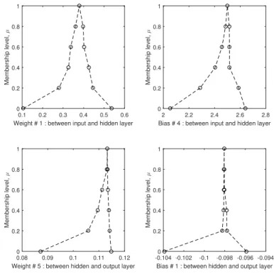
Alvisi and Franchini (2011) proposed a method to create a FNN, where the weights and biases, and by extension the output, of the neural network are fuzzy numbers rather than crisp (non-fuzzy) numbers. These fuzzy numbers quantify the total uncertainty of the calibrated parameters. While fuzzy set theory based applications of ANN have 5

been limited in hydrology, most have used fuzzy logic, e.g. the widely used Adaptive Neuro-Fuzzy Inference System, where automated IF-THEN rules are used to create crisp outputs (Abrahart et al., 2010; Alvisi and Franchini, 2011). Thus, the advantage of fuzzy outputs is that it provides the uncertainty of the predictions as well, while the fuzzy parameters reflect the uncertainty in the model structure. This uncertainty 10

quantification can be used to by end users to assess the value of the model output. In their FNN, the MLP model is presented in Eqs. (5) and (6) is modified to predict an interval rather than a single value for the weights, biases and output, corresponding to

anα-cut interval (at a defined membership levelµ). This is repeated for severalα-cut

levels, thus building a discretised fuzzy number at a number of membership levels. This 15

is done by using a stepwise, constrained optimisation approach:

h

yL_iyU_i i=_f_HIDh_WL

IHW U IH

i

x_i+h_BL

HB U H

i

(10)

h

zL_izU_i i=_f_OUTh_WL

HOW U HO

i

×hyL_iyU_i i+h_BL

OB U O

i

(11)

where all the variables are as described as before, and the superscripts “U” and “L”

represent the upper and lower limits of theα-cut interval, respectively. The constraints

20

(24)

HESSD

12, 12311–12376, 2015

network

Title Page Abstract Introduction Conclusions References Tables Figures ◭ ◮ ◭ ◮ Back Close

Full Screen / Esc

Printer-friendly Version Interactive Discussion Discussion P a per | Discussion P a per | Discussion P a per | Discussion P a per | min n X

i=1

zL_i −zU_i !

1

n

X

i=1

(δi)> PCI (12)

δi =

(

1, ifzL_i < ti <z U i

0, otherwise

wheretis that target (observed data) andPCIis a predefined percentage of data. Alvisi

and Franchini (2011) definedP to be 100 % atµ=_{0, 99 % at}_µ=_{0.25, 95 % at}_µ=_0.5

5

and 90 % atµ=_{0.75. This algorithm was built starting at}_µ=_{0 and moving to higher}

membership levels to maintain convex membership functions of the generated fuzzy numbers by using the results of the previous optimisation as the upper and lower limit

constraints for the proceeding optimisation. Lastly, at µ=_{1, the interval collapses to}

a singleton, represent the crisp results from non-fuzzy ANN. Therefore, these α-cut

10

intervals of the FNN output quantify the uncertainty around the crisp prediction, within

which is expected to containPCIpercentage of data.

In this research, this method is modified in two ways. First, the inputs x are also

fuzzy numbers, which means that Eqs. (10) and (11) are revised as follows:

h yL iy U i i

=_f_HIDh_WL

IHW U IH

i ×hxL

ix U i

i

+h_BL

HB U H i (13) 15 h

zL_izU_i i=_f

OUT

h

WL_HOWU_HOi×hyL_iyU_i i+h_BL

OB U O

i

. (14)

Note that now the input vector is represented by its upper and lower limits. The ma-jor impact on this is that the training algorithm for the FNN needs to accommodate

this fuzzy α-cut interval, which requires the implementation of fuzzy arithmetic

prin-ciples (Kaufmann and Gupta, 1985). The cost function for the optimisation remains 20

(25)

HESSD

12, 12311–12376, 2015

network

Title Page

Tables Figures

◭ ◮

Back Close

Full Screen / Esc

Discussion

P

a

per

|

Discussion

P

a

per

|

Discussion

P

a

per

|

Discussion

P

a

per

|

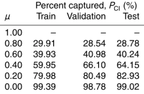
The second modification of the original algorithm is related to the selection of the

percent of data included in the predicted interval (PCI). In the original, the selection

is arbitrary and end-users of this method may be interested in the events that are

not included in the selected PCI. Thus, a full spectrum of possible values for a given

prediction is required. Thus, the Alvisi and Franchini (2011) approach is further refined 5

by utilising the same relationship between probability and possibility that was used to define the input fuzzy numbers, giving a more objective means of designing FNNs with fuzzy weights, biases and output.

In the adopted possibility-probability framework, the interval [a b]_α created by the

α-cut at aµ=_α_{implies that:}

10

[p(x < a)+_p₍_{x > b}_)]=_α_. ₍₁₅₎

This can be used to calculate the probability:

[p(a < x < b)]=₍₁₋_α_). ₍₁₆₎

This means that there is a probability of (1−α) that the random variablex falls within

the interval [a b]α. In other words theα-cuts of a possibility distribution (at anyµ)

cor-15

respond to the (1−α) confidence interval of the probability distribution of the same

variable (Serrurier and Prade, 2013). This principle is used to select the diﬀ_erent_P _for

the optimisation constraints rather than the predeterminedPCI selected by Alvisi and

Franchini (2011) These are shown in Table 2.

Note that for practical purposes, P_CI was selected as 99.50 % at µ=_{0 to prevent}

20

over-fitting. The implication of this selection is that at µ=_0, _nearly-all _{the observed}

data should fall within this predicted FNN interval, reflecting the highest uncertainty

in the prediction. The uncertainty decreases as µincreases. For the µ=_{1 case the}

values of the weights and biases were determined to be the mid-point of the interval

atµ=_{0.8 to maintain convexity of the produced fuzzy numbers, and the di}ﬃ_{culty in}

25