David C. Wyld et al. (Eds) : NETCOM, NCS, WiMoNe, CSEIT, SPM - 2015
pp. 21–37, 2015. © CS & IT-CSCP 2015 DOI : 10.5121/csit.2015.51603
Xinmin Tang
1, Shangfeng Gao
1, Songchen Han
2, Zhiyuan Shen
1,
Liping Di
2and Binbin Liang
21
College of Civil Aviation,
Nanjing University of Aeronautics and Astronautics, Nanjing, China
tangxinmin@nuaa.edu.cn
2
School of Aeronautics & Astronautics,
Si Chuan University, Chengdu, China
hansongchen@nuaa.edu.cn
A
BSTRACTIn view of the inherent defects in current airport surface surveillance system, this paper proposes an asynchronous target-perceiving-event driven surface target surveillance scheme based on the geomagnetic sensor technology. Furthermore, a surface target tracking and prediction algorithm based on I-IMM is given, which is improved on the basis of IMM algorithm in the following aspects: Weighted sum is performed on the mean of residual errors and model probabilistic likelihood function is reconstructed, thus increasing the identification of a true motion model; Fixed model transition probability is updated with model posterior information, thus accelerating model switching as well as increasing the identification of a model. In the period when a target is non-perceptible, prediction of target trajectories can be implemented through the target motion model identified with I-IMM algorithm. Simulation results indicate that I-IMM algorithm is more effective and advantageous in comparison with the standard IMM algorithm.
K
EYWORDSsurface surveillance, geomagnetic sensor technology, I-IMM, target trajectory, tracking and prediction
1. I
NTRODUCTION
Encountering increasingly serious problems regarding safety and efficiency on the airport surface, ICAO proposed an Advanced Surface Movement Guidance and Control System (A-SMGCS) [1]. The system performs surveillance, routing, guidance and control on a moving target using various sensor technologies, wherein surveillance is defined as the most important function in A-SMGCS[2].
devices. These three systems, however, have the following inherent defects: (1) SMR is susceptible to factors like building block, ground clutters and weather; (2) MALT and ADS can only monitor a target equipped with a transponder, but not a non-cooperative target on the surface; (3) These three surveillance approaches feature in low trajectory update rate, communication delay and high cost. The study of surface moving surveillance system based on event-driven non-cooperative can fundamentally solve the above-mentioned defects. Honeywell developed a dual infrared/magnetic sensor, and thousands of such sensors are equipped at airports for detection of the aircraft [3]. Chartier et al. proposed that the position of the aircraft could be determined though the information of coil sensor installed on the boundary of the airfield pavement segmentation[4]. K. Dimitropoulos et al. proposed to detect a magnetic target using a magnetic sensor network[5]. Schonefeld J et al. conducted comprehensive analysis on the performance of runway intrusion prevention system, XL-RIAS, based on distributed sensors, and testified that the response rate thereof is faster than that of ASDE-X [6].
Trajectory tracking and prediction of a target on the airport surface is a main function of the surface surveillance system. Two main trajectory tracking and prediction algorithms are studied. One is algorithm based on parameter identification in aircraft dynamics and kinemics models, wherein Gong studied taxing velocity and acceleration characteristics of the aircraft, and obtained kinematics trajectory model using regression analysis [7]; Capoozi et al. analyzed historical data of surface surveillance and excavated parameters of kinematics equation model [8]; Rabah W et al. employed high-gain observer and variable structure control method to perform output feedback tracking on nonlinear system, with effects of tracking uncertain system being undesirable[9]. Another is algorithm based on optimal estimation theory, wherein conventional Kalman filters like
α β
- andα β γ
- - are single model tracking algorithms, which are not suitable for the variety and uncertainty of target motion on the surface[10]; Farina et al. applied the restricted information to IMM model set self-adaption in consideration of peculiarity of a target motion on the airport surface, thus improving the tracking precision [11]; Gong Shuli et al. applied VS-IMM algorithm to the surface target tracking in combination with the airport map [12].2. S
URFACE
T
ARGET
S
URVEILLANCE
S
CHEME
B
ASED
ON
G
EO-
MAGNETIC
S
ENSOR
T
ECHNOLOGY
2.1. Surface target surveillance scheme
In general, moving targets on the airport surface comprise aircraft and special vehicles, which are relatively large ferromagnetic objects, generating disturbance to the surrounding magnetic field during their moving, thereby targets can be detected by the geomagnetic sensor with an anisotropic magnetoresistance effect according to the disturbance[13]. Combination of geomagnetic sensor and event-driven wireless sensor network can achieve high precision, small volume, low cost, no need for wiring and deployment flexibility, without affecting the surface surveillance performance. The surface moving target surveillance scheme based on the magnetic sensor technology is as shown in Figure 1.
Figure1. Surveillance scheme for targets on the surface
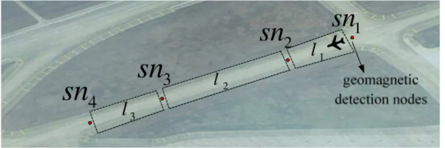
2.2. Node deployment and runway section information
in combination with surface restrictions as is shown in Figure 2 (taking a taxiway section as an example).
2
l
3
l
1
sn
2sn
3
sn
4
sn
1
l
Figure 2. Node deployment
The taxiing route of a moving target on the surface is divided into different sections,
{
1, ,
2 3}
L
=
l l l
. A target mostly maintains single motion characteristics in different sections. Forinstance, the aircraft maintains accelerated motion during section
l
1, constant motion duringsection
l
2, and decelerated motion during sectionl
3. Geomagnetic detection nodes{
1,
2,
3,
4}
SN
=
sn sn sn sn
, are deployed at the cut-off rule of the adjacent sections. Each sectioncomprises four parameters. For instance, sectionican be defined as
(
l sn sn
i,
i,
i+1,
long
i)
, where il
denotes number,sn
idenotes start node,sn
i+1denotes terminal node, andlong
idenotes length. The section information is preserved in geomagnetic detection nodes for distributed computation after nodes perceive a target. In above-mentioned deployment, nodes can accurately perceive the target position as a target passes through them and modify the previous position information, and the velocity information can also be modified instantaneously via the target velocity obtained from nodes.3. I-IMM-B
ASED
S
URFACE
T
ARGET
T
RACKING
AND
P
REDICTION
A
LGORITHM
In the surface surveillance scheme based on geomagnetic sensor technology, a target is in a perceptible state as it passes through nodes, which provide the velocity information. The data volume, however, is not large and can only be seen as small data samples. When a target completely detaches from nodes, it would be in an imperceptible state when moving in the section between nodes. Accordingly, the target tracking and prediction algorithm put forward in this paper needs to satisfy requirements as follows: When a target is perceptible, the real-time tracking is performed using the observed velocity information and the target motion model is accurately identified; When a target is not perceptible, extrapolated prediction is performed on trajectories thereof using the identified motion model.
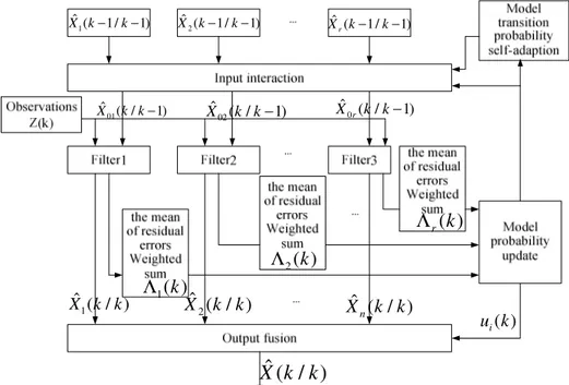
3.1. I-IMM algorithm
probability is updated for self-adaption using model posterior probability, thus accelerating model switching as well as increasing the identification of a model. The schematic diagram of I-IMM algorithm is as shown in Figure 3. This algorithm comprises the following 5 steps:Input interaction; Kalman filter; Model probability update; Model transition probability self-adaption; Output fusion.
1
ˆ ( 1 / 1)
X k− k− X kˆ (2 −1 /k−1) X kˆ (r −1 /k−1)
01 ˆ ( / 1)
X k k− Xˆ ( /02 k k−1) Xˆ ( /0r k k−1)
1
ˆ ( / )
X k k 1 X k kˆ ( / )2 X k kˆ ( / )n ( )k
Λ
2( )k
Λ
( )
r
k
Λ
( ) i
u k
ˆ ( / )
X k k
Figure 3. Schematic diagram of I-IMM algorithm
3.1.1. Input interaction
Assuming that a model set consists of
r
motion models, the state estimation value and covariancematrix of each model at time
k
−
1
are respectively as follows: X kˆ (j−
1|k−
1)andP kˆ (j−
1|k−
1),j=1, 2,L ,r.
After interaction, the input in model jat time
k
is expressed as follows:0
1
ˆ ( 1| 1) r ˆ ( 1| 1) ( 1| 1)
j i ij
i
X k k X k k u k k
=
− − = − − − − (1)
0
1
0
ˆ
(
1|
1)
(
1|
1){ (
ˆ
1|
1)
ˆ
ˆ
[
(
1|
1)
(
1|
1)] }
r
j ij i
i
T
i j
P
k
k
u k
k
P k
k
X k
k
X
k
k
=
−
−
=
−
−
−
−
+
−
−
−
−
−
(2)
Where, the mixture probability after input interaction is defined as:
( 1| 1) ( 1) /
ij ij i j
Where,
1
( 1)
r
j ij i
i
c p u k
=
= − ,pijdenotes model transition probability, and u ki(
−
1) denotesprobability in model i at time
k
−
1
.3.1.2. Kalman filter
Kalman filter consists of prediction process and update process. The prediction process is expressed by Eq. (4) and Eq. (5):
0
ˆ ( | 1) ˆ ( 1| 1)
j j j
X k k
−
=
F X k−
k−
(4)T 0
ˆ( | 1) ˆ ( 1| 1)
j j j j
P k k
−
=
F P k−
k−
F+
Q (5)In the above equations, Fj is the model state transition matrix; Q is the noise covariance in
each model during the estimation.
Residual sequence and covariance matrix are:
ˆ
( ) ( ) ( | 1)
j j j
r k
=
Z k−
HX k k−
(6)T ˆ
( ) ( | 1)
j j
S k
=
HP k k−
H+
R (7)In the above equations, Z kj( ) is the observed value for the time
k
; H is the observationmatrix; R is the noise covariance of observation.
Kalman filter gain matrix is:
1 ˆ
( ) ( | 1) T ( )
j j j
K k
=
P k k−
H S− k (8)State estimate and covariance matrix update are expressed as follows:
ˆ ( | ) ˆ ( | 1) ( ) ( )
j j j j
X k k
=
X k k−
+
K k r k (9)T ˆ ( | ) ˆ ( | 1) ( ) ( | 1) ( )
j j j j j
P k k
=
P k k−
−
K k S k k−
K k (10)3.1.3. Model probability update
In IMM algorithm, maximum likelihood function in model jis as given in Eq. (11):
1
1
1
( )
exp{
( )
( ) ( )}
2
2
( )
T
j j j j
j
k
r
k S
k r k
S k
π
−
Λ
=
−
(11)As can be seen from the Eq. (11), it is assumed that the motion model set can contain all motion models of a target during the operation in IMM algorithm. However, due to the factors like uncertainty of the motion of a surface target, surface restrictions and spot dispatch, the target motion model may exceed the model set in the algorithm. Therefore, innovation information is no longer considered to obey Gaussian distribution, in which mean value is zero and variance is
( )
j
Let assume the true motion model of a surface moving target to be as follows:
( ) ( 1) ( 1) ( 1)
T T T T
X k
=
F k−
X k−
+
w k−
(12)( ) T( ) T( )
Z k
=
HX k+
v k (13)Define the model state transition matrix error as follows:
j T j
F F F
∆ = − (14)
Define the state estimation error as follows:
ˆ
( 1) ( 1| 1) ( 1| 1)
j T j
e k
−
=
X k−
k−
−
X k−
k−
(15)Expression for the state estimation error after input interaction is obtained:
0 0
1 ˆ
( 1) ( 1| 1) ( 1| 1) ( 1| 1) ( 1)
r
j T j ij i
i
e k X k k X k k u k k e k
=
− = − − − − − = − − − (16)
Given by Eq. (6) and Eq. (12), the residual error is obtained:
0 ˆ
( ) ( ) ( ) ( 1| 1)
j T T j j
r k
=
HX k+
v k−
HF X k−
k−
(17)Given by Eq. (12) and Eq. (15), the residual error is obtained:
0 ˆ0
( ) ( -1) ( -1| -1) ( ) ( )
j T j j j T T
r k
=
HF e k+
H F X∆
k k+
Hw k+
v k (18)Mean value obtained from Eq. (18) can be expressed as follows:
0 ˆ0
( ) ( 1) ( -1| -1)
j T j j j
r k
=
HF e k−
+
H F X∆
k k (19)Where, 0
1
( 1) ( 1| 1) ( 1)
r
j ij i
i
e k u k k e k
=
− = − − − (20)
Because of the uncertainty of the true motion model of a surface target, the quantization of FT
and∆Fjin Eq. (19) cannot be performed, causing the mean of residual errors not to be obtained.
To solve this problem, the true motion model of a target is assumed to be j, and weighted sum is
performed on another model in the model set to obtainr kj( ).
(
)
0 0
1
ˆ
( ) ( 1) ( -1| -1) 1| 1
r
j j i i j i i
i
r k HF e k H F X k k u k k
=
= − + ∆ − − (21)
Where, ∆Fi =Fj−Fi,and 0
1
( 1) ( 1| 1) ( 1)
r
i in n
n
e k u k k e k
=
− = − − − .
Then, maximum likelihood function in modeljat time
k
can be given as:1
1 1
( ) exp ( ) ( ) ( ) ( ) ( )
2 2 ( )
T
j j j j j j
j
k r k r k S k r k r k
S k
π
−
( )
( )
(
)
( )
11
1 /
r
j j ij i j j
i
u k k p u k k c c
c =
= Λ − = Λ (23)
Where,
( )
1
r
j j
j
c
k c
=
=
Λ
(24)3.1.4. Model transition probability self-adaption
In IMM algorithm, because of the uncertainty of the target maneuver and the distortion of the prior information, the fixed model transition probabilitypij fails to reflect the true motion model
of a target, and switching velocity between models is also delayed during the target maneuver. Given that the observed velocity is small sample information, applying the fixed model transition probabilitypijmay likely cause the target motion model hard to be identified or even not to be
identified. Therefore, the model transition probabilitypijis updated using posterior information in
I-IMM algorithm to solve this problem.
Assuming that the probability in model jat time
k
−
1
isu
j(
k
−
1
)
and at timek
isu
j( )
k
, theprobability differential value of the same model at adjoining times reflects the change in the matching degree between model jand the true motion model. The rate of change of the posterior probability in model jcan be defined as:
( )
( )
(
1
)
j j j
u
k
u
k
u
k
∆
=
−
−
(25)Let the model transition probability from model i to model jat time
k
−
1
bep
ij(
k
−
1
)
, andupdate
p
ij(
k
−
1
)
using∆
u
j( )
k
, then the expression is obtained:( )
exp(
( )
)
(
1)
ij j ij
p′ k = ∆u k p k− (26)
Model transition probability needs to satisfy basic properties as follows:
1
0
1, ,
1, 2,
,
1
ij
r
ij j
p
i j
r
p
=
<
<
=
=
L
(27)
Then, normalization needs to be performed on
p
ij′
( )
k
, and the transition probabilityp
ij( )
k
canbe obtained:
( )
( )
( )
( )
(
)
(
)
( )
(
)
(
)
1 1 exp 1 exp 1 j ij ijij r r
ij j ij
j j
u k p k p k
p k
p k u k p k
As can be seen from Eq. (28), updated
p
ij( )
k i
,
=
1, 2,
L
,
r
increases as the transition of modelfrom modelito model j, when the posterior information
∆
u
j( )
k
increases, thus model jplays acritical role in input interaction at next time period.
3.1.5. Output fusion
Interactive output results at time
k
are expressed as follows:(
)
(
) ( )
1
ˆ
|
rˆ
|
j j
j
X k k
X
k k u
k
=
=
(29)(
)
( )
{
(
)
(
)
(
)
(
)
(
)
T}
1
ˆ
|
r|
ˆ
|
ˆ
|
ˆ
|
ˆ
|
j j j j
j
P k k
u
k
P k k
X
k k
X k k
X
k k
X k k
=
=
+
−
−
(30)3.2. Trajectory prediction of targets not perceptible
A target would be not perceptible as moving in the section between two adjacent nodes, requiring memory tracking of target trajectories using extrapolated prediction.
At last moment of the period when a target is perceptible, I-IMM provides identification of each model in the model set, namely, model posterior probability
u
j( )
k
,
j
=
1, 2,
L
,
r
. Then given by the self-adapting model transition probabilityp
ij( )
k
, the expression for prediction probability ofeach model in the model set when a target not perceptible at time
k
+
1
can be obtained:(
)
( )
1
1| ( ) , 1, 2, ,
r
j i ij
i
u k k u k p k j r
=
′ + = g = L (31)
At the same time, posterior probability of each model needs to satisfy the following properties:
1
0
1,
1, 2,
,
1
j
r
j j
u
j
r
u
=
<
<
=
=
L
(32)
Then, normalization needs to be performed on posterior probability of each model predicted from Eq. (31), and model posterior probability at moment
k
+
1
is obtained:(
)
(
)
(
)
11|
1|
=
1|
j j r j ju
k
k
u
k
k
u
k
k
=
′
+
+
′
+
(33)
After substituting state predicted value, Xˆj
(
k+1|k)
and prediction model probability,(
1|
)
j
u
k
+
k
of each model into Eq. (29), state predicted value of the period when a target is not(
)
(
) (
)
1ˆ
1|
rˆ
1|
1|
j j
j
X k
k
X
k
k u
k
k
=
+
=
+
+
(34)By performing extrapolated prediction on surface target trajectories using state predicted value obtained from Eq. (34), memory tracking and prediction can be implemented on a target not perceptible.
4. S
IMULATION
AND
A
NALYSIS
4.1. Preparation for simulation
This paper presents, taking aircraft passing through a certain geomagnetic detection node on the taxiway for an example, IMM algorithm and I-IMM algorithm are compared through Monte Carlo simulation, regarding the performance of trajectory tracking of the aircraft perceptible and trajectory prediction of the aircraft not perceptible.
According to the motion characteristics of the aircraft on the surface, the aircraft motion can be expressed by a model set comprising constant velocity (CV) model, constant acceleration (CA) model and constant jerk (CJ) model. State transition matrixes of three models are respectively expressions as follows:
1 0 0
0 1 0 0
0 0 0 0
0 0 0 0
CV
T
F = ,
2
1 0
2
0 1 0
0 0 1 0
0 0 0 0
CA
T T
T
F = ,
2 3
2
1
2
6
0
1
2
0
0
1
0
0
0
1
CJ
T
T
T
T
F
T
T
=
Where, T is the interval of sampling. Motion state vector of the aircraft is , and
observation matrix is
H
=
[
0 1 0 0
]
.In the period when aircraft is perceptible, the process of the aircraft operation is as follows:(1) Performing CJ at 0.3m s/ 3from 0 to 4.5 seconds; (2) Performing CA at 0.45m s/ 2from 4.58 to 12 seconds; (3) Performing CV at the velocity obtained from step (2) from 12 to15 seconds.
In the period when aircraft is not perceptible, it maintains CV for about 30 seconds at the velocity obtained from step (3) and then operates to the next detection node.
Figure 4. Actual position of the aircraft
The simulation parameters selection is as follows: Noise covariance in each model during the
estimation is
0.01 0 0 0
0 0.01 0 0
0 0 0.01 0
0 0 0 0.01
Q= ; Noise covariance of velocity observation is
0.15
R
=
; the interval of sampling isT
=
0.3
s
; Initial model probabilities of CV model,CA model and CJ model are respectively 0.4,0.3 and 0.3; Initial model transition matrix can begiven as:
0.9
0.05 0.05
0.05
0.9
0.05
0.05
0.05
0.9
markov
P
=
.4.2. Simulation results and analysis in perceptible period
Simulation results in the period when the aircraft is perceptible are as displayed in Figure 5 to 8.
Figure 6. Velocity tracking
Figure 7. Acceleration tracking
Figure 8. Jerk tracking
0 1.5 3 4.5 6 7.5 9 10.5 12 13.5 15
0 0.2 0.4 0.6 0.8 1 1.2 1.4
Time/s
A
c
c
e
le
ra
ti
o
n
/m
/s
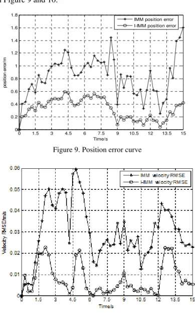
Figure 5 to 8 illustrate the excellence of I-IMM algorithm when used to track the motion state of the aircraft. Fig. 5 and 6 demonstrate that compared with IMM algorithm, the position and velocity tracked with I-IMM algorithm are more approximate to the actual position and velocity of the aircraft. To show the advantage of I-IMM more manifestly, the position error curve and velocity root-mean-square error(RMSE) curve of I-IMM and IMM algorithm are respectively plotted, as shown in Figure 9 and 10.
Figure 9. Position error curve
Figure 10. Velocity RMSE curve
Figure 9 shows maximum position error using IMM algorithm is 1.600m, while using I-IMM algorithm is only 0.600m. Figure 10 shows maximum RMSE error using IMM algorithm is 0.059m/s, while using I-IMM algorithm is 0.023m/s. As can be seen from the result, the tracking precision is well improved when using I-IMM algorithm.
Figure 11 presents the selection probability curves of CV, CA and CJ models when IMM and I-IMM algorithm are respectively employed. Figure 11 demonstrates that I-IMM algorithm cannot identify each motion model very clearly, and three selection probability curves intersect intensely. For instance, in constant accelerating phase, IMM algorithm’s maximum identification
0 1.5 3 4.5 6 7.5 9 10.5 12 13.5 15
0 0.2 0.4 0.6 0.8 1 1.2 1.4 1.6 1.8
Time/s
p
o
s
it
io
n
e
rr
o
r/
m
degree of CA model is 0.710; Comparatively, I-IMM algorithm can largely improve the identification degree. In constant jerking phase, the maximum identification degree of CJ model is 0.987, while in constant accelerating phase, the maximum identification degree of CA model can reach to 0.987, and in constant velocity phase, the maximum identification degree of CV model is 0.987. As for model switching, the switching velocity in I-IMM algorithm is much faster than that in IMM algorithm. In IMM algorithm, it takes 2.4 seconds to switch from CJ model to CA model, and 1.8 seconds from CA model to CV model. In comparison, when employing I-IMM algorithm, it only takes 0.9 seconds to switch from CJ model to CA model, and only 0.9 seconds from CA model to CV model.
Figure 11. Selection probability in IMM and I-IMM
4.3. Simulation results and analysis in imperceptible period
Simulation results of trajectory prediction in the period when the aircraft is not perceptible are as displayed in Figure 12 and 13.
Figure 13. Position prediction error
Figure 12 illustrates that the deviation between the aircraft position predicted with either IMM or I-IMM algorithm and the real position increases with the increase of the running time. Figure 13 illustrates that at the last moment of position prediction, the position prediction error is accumulated to 9.790m when IMM algorithm is used, while only to 2.160m when I-IMM algorithm is used. It is apparent that I-IMM algorithm outperforms IMM algorithm in terms of trajectory extrapolated prediction, particularly in the period when the aircraft is not perceptible.
5. C
ONCLUSIONS
In view of the inherent defects in current surface surveillance system, this paper proposes a asynchronous target-perceiving-event driven surface moving target surveillance scheme based on the geomagnetic sensor technology. Furthermore, a surface moving target tracking and prediction algorithm is given based on I-IMM, which is improved on the basis of IMM algorithm in the following aspects: Weighted sum is performed on the mean of residual errors and model probabilistic likelihood function is reconstructed, thus increasing the identification of a true motion model; Model transition probability is updated for self-adaption with model posterior probability, thus accelerating model switching as well as increasing the identification of a model. At last, this paper presents simulation results of target tracking and prediction in both periods when a target is perceptible and not perceptible using two algorithms, demonstrating that the I-IMM algorithm is more effective than I-IMM algorithm, particularly when a target is not perceptible.
A
CKNOWLEDGEMENTSR
EFERENCES[1] International Civil Aviation Organization. Doc. 9830-AN/452 Advanced surface movement guidance and control systems(A-SMGCS) manual. Montreal: ICAO, 2004.
[2] EUROCONTROL, Development and Validation of Improvement of Runway Safety Net (A-SMGCS Level 2) by Electronic Flight Strips–D16 Cost Benefit Analysis. Toulouse, EUROCONTROL, 2010.
[3] Stauffer D, French H & Lenz J. (1993) “A multi-sensor approach to airport surface traffic tracking”, Digital Avionics Systems Conference, pp430-432.
[4] Chartier, E. & Hashemi, Z. (2001) “Surface surveillance systems using point sensors and segment-based tracking”, Digital Avionics Systems, 2001. DASC. 20th Conference, Vol. 1, pp2E1/1 - 2E1/8.
[5] Dimitropoulos, K., Grammalidis, N., Gragopoulos, I., Gao, H., Heuer, T.& Weinmann, M., et al. (2006) “Detection, tracking and classification of vehicles and aircraft based on magnetic sensing technology”, Proceedings of World Academy of Science Engineering & Technology, Vol. 4, No. 1, pp195-200.
[6] Schonefeld J, & Moller D P F. (2012) “Fast and robust detection of runway incursions using localized sensors”, Multisensor Fusion and Integration for Intelligent Systems (MFI), pp33 - 39.
[7] Gong, C. (2009) “Kinematic airport surface trajectory model development”, 9th AIAA Aviation Technology, Integration, and Operations Conference (ATIO) , pp175-179.
[8] Capozzi, B., Pledgie, S. & Kistler, M. (2010) “Surface Trajectory Characterization Report”, NRA Contact NNA09DA89C, pp1-20.
[9] Aldhaheri, R. W. & Khalil, H. K. (1996) “Effect of unmodeled actuator dynamics on output feedback stabilization of nonlinear systems”, Automatica, Vol. 32, No. 96, pp1323–1327.
[10] Zhou Hongren, Jing Zhongliang & Wang Peide. (1990) “Tracking Maneuvering Targets”, Beijing: National Defense Industry Press.
[11] Farina A, Ferranti L & Golino G. (2003) “Constrained Tracking Filters For A-SMGCS”, Information Fusion, 2003. Proceedings of the Sixth International Conference,Vol. 1, pp414-421.
[12] Gong Shuli, Tao Cheng & Wang Bangfeng. (2012) “A-SMGCS Surface Moving Target Tracking Based on VS-IMM Algorithm”, Transactions of Nanjing University of Aeronautics & Astronautics, Vol. 44, No. 1, pp118-123.
[13] Klausner A, Tengg A & Rinner B. (2007)“Vehicle Classification on Multi-Sensor Smart Cameras Using Feature- and Decision-Fusion”, First Acm/ieee International Conference on Distributed Smart Cameras, pp67 - 74.
A
UTHORSDr. Xinmin Tang was born in 1979. He obtained his Ph.D. in Mechanical Engineering at the Harbin Institute of Technology in 2007. He is currently an Associate Professor in the College of Civil Aviation at Nanjing University of Aeronautics and Astronautics. His research interests include (1) Petri Net and Discrete Event Dynamic System theory; (2) Hybrid System Theory.
Shangfeng Gao was born in 1990. He holds a Master Degree in Engineering from the College of Civil Aviation at Nanjing University of Aeronautics and Astronautics. His major course is Transportation planning and management. His research interests include Advanced Surface Movement Guidance and Control System (A-SMGCS).
Dr. Songchen Han was born in 1964. He obtained his Ph.D. in Engineering at Harbin Institute of Technology. He is currently a professor in Sichuan University in China. His research interests include (1) next generation air traffic management system (2) air traffic planning and simulation.
Dr. Zhiyuan Shen is an assistant professor at college of civil aviation, Nanjing University of Aeronautics and Astronautics (NUAA). He received Ph.D in control science and engineering from the Harbin Institute of Technology, China. Between 2010 and 2012, he was a visiting scholar in Electrical and Computer Engineering at Georgia Institute of Technology, Atlanta. His current research interest includes ADS-B technique and 4D trajectory prediction.
Liping Di was born in 1964. She obtained his Bachelor Degree in Aircraft Control at the Harbin Institute of Technology in China. She is currently a teacher in Sichuan University. Her research interest is aircraft control.