Abstract—In this work, Neural Networks (NN) approach was proposed to deal with abrasiveness behavior of thermal coal. Back-propagation neural network (BPNN) and Generalized regression neural network (GRNN) techniques were employed to assess the Abrasive index (AI) of coal to mineral. The multivariate statistical results revealed that the BPNN and GRNN models were successfully developed to model the abrasiveness characteristics of thermal coal with the coefficient of determination, R2 = 0.9003 for BPNN and R2 = 0.937 for GRNN. These good results indicated that the NN techniques were capable of accurately modeling the abrasiveness characteristics of coal.
Keywords: Abrasive index, back-propagation neural network, coal, generalized regression neural network.
I. INTRODUCTION
OAL is a combustible, organic rock, which is composed mainly of carbon, hydrogen and oxygen. Coal is primarily used as a solid fuel to produce electricity and heat through combustion. When coal is used for electricity generation, it is usually grinded to an efficient burnable size in a mill and then burned in a furnace with a boiler. During grinding, frictions occur, cause abrasive wear or erosion on the critical components and thereby affect the performance of power plant. It is therefore important to assess the relative abrasion characteristics of thermal coal by selecting the right type of materials for grinding and burning of the coal [1].To study the abrasion of coals, an index namely abrasion index (AI) which has been used to assess the abrasive nature of the thermal coal was established first by Yancey, Geer and Price (YGP) in 1951 using YGP test rig. Over the years there have been some modifications to this method by both mining houses and coal users which have resulted in inconsistent and conflicting results [2]. AI was then measured using different methods, which include the AI tester pot using four iron blades as cutting elements [3]. Reference [4] revealed that two and three-body abrasive wear is not only concerned with hard material, as material of less hardness than the concerned metal blades can still cause material wear. Reference [3] revealed that the effects of
Manuscript received July 07, 2016; revised July 22, 2016. This work was supported by the Centre for Renewable Energy and Water, Vaal University of Technology, South Africa.
J. Kabuba is with the Centre for Renewable Energy and Water, Department of Chemical Engineering, Vaal University of Technology, Private Bag X021, Vanderbijlpark 1900, South Africa. Tel. +27 16 950 9887; fax: +27 16 950 6491; e-mail: johnka@ vut.ac.za.
particles that are less hard than the cutting blades are inconsistent in comparison to harder minerals. To improve the prediction of abrasiveness of thermal coal, it is important to understand the nature and properties of the mineral matters in a coal that would contribute to abrasive wear. Most of the empirical equations available in literature [5]-[9] for predicting AI of coal, are based on linear assumptions which may lead to erroneous estimations and do not take into consideration most of the relevant factors. To achieve this, Neural Network (NN) based predictive techniques was suggested to understand the nonlinear relationships and thereby achieving ability to predict accurately. Reference [10] used non-linear multivariable regression and NN to find the correlation between Hardgrove grindability index and the proximate analysis of chemise coals. Reference [11] also used NN to studies the relationship between petrography and grindability for Kentucky coals. To our knowledge, this is the first time that NN has been used to predict the abrasive index of the coal. The objective of this study is to investigate the possibility for the prediction of abrasiveness characteristics of thermal coal abrasive index using neural network.
II. MATERIALS AND METHODS A. Experimental Data
The coal samples used in this study was sourced from different colliers in South Africa. These samples were analyzed for both their chemical and physical characteristics based on the premise that they can contribute information that can make it possible for this study to adequately reveal coal constituents that cause abrasion during grinding. The abrasion index tester pot was used to determine AI of the coal samples. A Perkin-Elmer simultaneous thermogravimetric analyzer (STA 6000) equipped with Pyris manager software was used to determine the proximate analyses that gives information about moisture and ash percentage, and petrographically determined minerals in the coal samples.
A multivariate statistical analysis was conducted, and from this analysis it was determined that four variables (Ash, Quartz, Pyrite and Moisture) were significant contributors to AI models.
B. Back-Propagation Algorithm (BPNN)
In this study, the first step was done to scale the inputs and targets within the range 0 and 1 in case the higher values would drive the training process and mask the
Application of Neural Networks Technique for
Predicting of Abrasiveness Characteristics of
Thermal Coal
John Kabuba, Member, IAENG
contribution of lower valued inputs, as well as to perform a principal component analysis to eliminate redundancy of the data set. In the second steps, the data set was divided into training, validation and testing subsets. The training set was used for updating the network weights and computing the gradient. The validation set was used for improving generalization. The testing set was used for validating the network performance. The data in each subset were selected randomly, and then a network was created. A total of ten training algorithms were conducted to simulate the test data. The performances of the network in each training process and the best network with the highest prediction performances were recorded.
C. Generalized Regression Neural Network (GRNN) The GRNN falls into the category of probabilistic NN that can solve any function approximation problem if sufficient data are available [12]. The additional knowledge needed to get the fit in a satisfying way is relatively small and can be done without additional input by the user. This makes GRNN a very useful tool to perform predictions of system performance in practice [12]. The expected value of the output y given the input vector x is given by:
dy y x f dy y x yf x y E ) , ( ) , ( (1)when the density
f
(
x
,
y
)
is not known, it must usually be estimated from a sample of observation of x and y. The probability estimatorg
(
x
,
y
)
in (2) is based on sample values xi and yi of the random variables x and y:
2 2 1 2 ) 1 ( 2 / ) 1 ( 2 ) ( exp 2 ) ( ) ( exp 1 2 1 ) , ( i n i i T i p p y y x x x x n y xg (2)
Where n is the number of sample observations, and p is the dimension of the vector variable x. A physical interpretation of the probability estimate
g
(
x
,
y
)
is that it assigns sample probability of width σ (smoothing factor) for each sample xi and yi, and the probability estimate is the sum of those sample probabilities [12]. The squared distance D between the input vector x and the training vector xi is defined as:)
(
)
(
2 i T i
i
x
x
x
x
D
(3) And the final output is determined by performing the integrations in (4). This result is directly applicable to problems involving numerical data.
n i i n i i i D D y g 1 2 2 1 2 2 2 exp 2 exp (4)
The smoothness parameter σ, considered as the size of the
neuron’s region, is a very important parameter of GRNN [12]. When σ is large, the estimated density is forced to be
smooth and in the limit becomes a multivariate Gaussian
with covariance σ2I (I = unit matrix), whereas a smaller
value of σ allows the estimated density to assume non -Gaussian shapes, but with the hazard that wild points may have a great effect on the estimate [12]. Therefore, a range of smoothing factors should be tested empirically to determine the optimum smoothing factors for the GRNN models [12]. In this study, NN toolbox 5.1 in Matlab 7.4 (R2007a) was used to develop the NN models.
D. Performance Indicators
The root mean square error (RMSE), mean absolute error (MAE), and coefficient of determination (R2) between the modelled output and measures of the training and testing data set are the most common indicators to provide a numerical description of the goodness of the model estimates. They are calculated and defined according to (5), (6) and (7), respectively [13]:
2 / 1 1 2 ) ( 1
N i i i P O NRMSE (5)
N i i i P O N MAE 1 1 (6)
N i i N i i A O A P R 1 2 1 2 2 ) ( ) ( (7)where N = number of observations, Oi = observed value,
Pi = predicted value, A = average value of the explained
variable on N observations.
RMSE and MAE indicate the residual errors, which give a global idea of the difference between the observed and predicted values. R2 is the proportion of variability in a data set that is accounted for by a model. When the RMSE and MAE are at the minimum and R2 is high (R2 ≥ 0.80), a model can be judged as very good [14].
III. RESULTS AND DISCUSSION A. BPNN Model Development
The development of a good BPNN model depends on parameters determined using error methods (RMSE, MAE and R2). Three important aspects (number of layers, neurons in the hidden layer and the type of activation functions for the layers) must be decided on the BPNN structure. A three-layer BPNN was constructed to determine if its prediction performance was superior to a two-layer network. Unfortunately, the results were almost the same. It is worth noting that the bigger network structure would need more computation and could cause overfitting of the data [15]. To optimize of the network, two neurons were used as an initial guess in the hidden layer. By increasing the number of neurons, the network gave several local minimum values and different error values were obtained for the training set.
TABLE I
DEPENDENCE BETWEEN THE NEURON NUMBERS AND RMSE
Number of Neurons RMSE
___________________________________________________________
2 0.134843
3 0.093658
4 0.054025
5 0.039396
6 0.000257
7 0.012368 8 0.013655
In Table I a gradual decrease was observed in the RMSE.
With 6 neurons in hidden layer, the MSE reached its minimum value of 0.000257. Hence, the neural network
containing 6 neurons in hidden layer was chosen as the best case. When the number of neurons exceeded 6 in hidden layer, the MSE showed an increase at 7 and 8 neurons. The networks are sensitive to the number of neurons in their hidden layers. The optimum number of neurons required is problem dependent, being related to the complexity of the input and output mapping, the amount of noise in the data, and the amount of training data available.
Sigmoid transfer functions are usually preferable to threshold activation functions because with sigmoid units, a small change in the weights produces a change in the output, which makes it possible to tell whether that change in the weights was good or bad. The following sigmoid transfer functions are often used for BPNN: Hyperbolic tangent sigmoid (tansig), log-sigmoid (logsig) and linear (purelin) transfer function. The tansig transfer function, which can produce both positive and negative values, tended to yield faster training that the logsig transfer function, which can produce only positive values. Table II summarizes the BPNN performance using different transfer functions, 6 neurons were used in the hidden layer for all transfer functions.
TABLE II
TRANSFER FUNCTION VERSUS R2
Transfer function R2
___________________________________________________________ Hidden layer Output layer
___________________________________________________________ logsig logsig 0.9054 logsig purelin 0.8609 logsig tansig 0.9102 tansig tansig 0.8909
tansig purelin 0.8346
All of the transfer function combination tested, the logsig transfer function at hidden layer and tansig transfer functions at output layer with the highest R2 (Table 2) were used in this work.
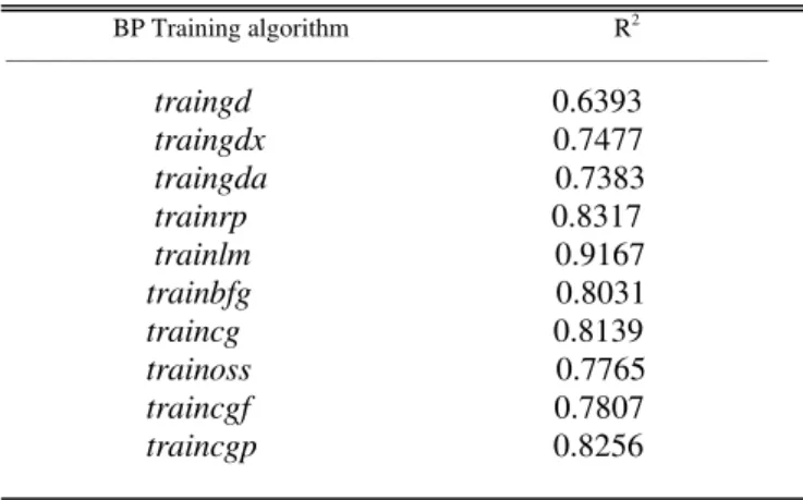
Once the BPNN was constructed, the weights were initialized and the network was ready for training. Ten different BP training algorithms were compared to select the best suited algorithm. For all BP training algorithms, a three-layer NN with a lo-sigmoid transfer function at hidden layer and a hyperbolic tangent sigmoid transfer function at output layer were used. For all BP training algorithms, 6 neurons were used in the hidden layer. Their characteristics deduced from the experiments are shown in Table III.
TABLE III
RESULTS USING DIFFERENT TRAINING ALGORITHMS
BP Training algorithm R2
________________________________________________________________________
traingd 0.6393 traingdx 0.7477 traingda 0.7383 trainrp 0.8317 trainlm 0.9167 trainbfg 0.8031 traincg 0.8139 trainoss 0.7765 traincgf 0.7807
traincgp 0.8256
The benchmark comparison showed that the traingd (gradient descent BP) algorithm had the lowest training speed compared to all other algorithms, follow by traingda (gradient descent BP with adaptive learning rate) with R2 = 0.7383, traingdx (gradient descent BP with momentum and adaptive learning rate), trainoss (one step secant BP), traincgf (conjugate gradient BP with Fletcher-Reeves), trainbfg (BFGS quasi-Newton), trainscg (scaled conjugate gradient BP), traincgp (conjugate gradient BP with Polak-Ribiere), trainrp (resilient BP). The trainlm (Levenberg-Marquardt) with the highest R2 was suitable as BP training algorithm.
The BPNN algorithm trainlm was developed using a three layer approach with a logsig transfer function at hidden layer and tansig transfer functions at output layer. This BPNN have six input neurons (moisture, ash, SiO2 and
pyrite) and one output neuron (AI) as shown in Fig. 1.
Fig. 1. BPNN structure uses in this study
by changing the number of layers, nodes, transfer function, and iteration number. The prediction of BPNN versus actual measure for all (training, testing and validation) is shown in Fig. 2.
Fig. 2. AI predicted by BPNN in testing process versus actual measured
B. GRNN Model Development
The smoothness factor σ is the only parameter which affects the GRNN performance by taking several aspects into account depending on the application the predicted output is used for [12]. For a prediction that is close to one of the training sample and a sufficiently small smoothness factor the influence of the neighboring training samples is minor. The contribution to the prediction is a lot smaller than the contribution of the training samples that are further away from the point of prediction can be neglected [12]. Due to the normalization the prediction therefore yields the value of the training sample in the vicinity of the each
training sample. For a bigger σ the influence of the
neighboring training samples cannot be neglected. The prediction then is influenced by more point and the
prediction is getting smoother. With even larger σ the
predicted curve will get flatter more smooth as well. In some cases this is desirable. For example when the available data include a lot of noise, then the prediction has to interpolate the data whereas if the data are correct [12]. GRNN has to fit the data more precisely and has to follow
each little trend the data makes. If the σ approaches infinity
the predicted value is simply the average of all the sample points. Due to the fact that data are not generally without measurement errors and that the circumstances change from application to application, there cannot be a right or wrong
way to choose σ. Table IV summarizes the results for GRNN model using different σ values. The σ value 0.05 can
fit data very closely, with higher R2 (0.951) value than when
using the larger σ, but the larger σ can make the function approximation smoother.
TABLE IV
GRNN USING DIFFERENT σ
σ R2
___________________________________________________________
0.05 0.951
0.10 0.908
0.25 0.725
0.50 0.660
1.00 0.523
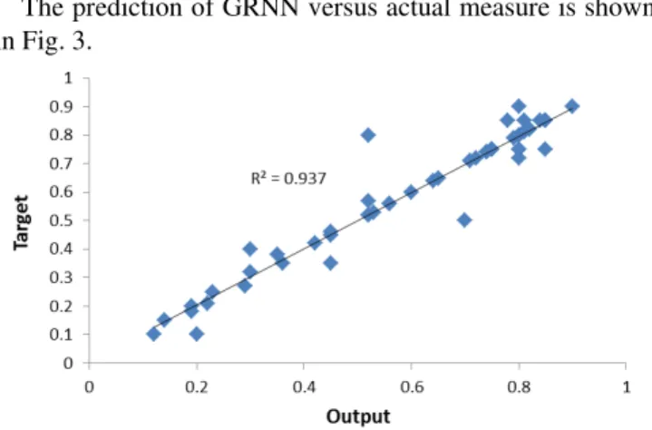
The prediction of GRNN versus actual measure is shown in Fig. 3.
Fig. 3. AI predicted by GNNN in training process versus actual measured
The proposed GRNN has three layers. To avoid overtraining, the spread constant was changed to allow testing data error became close the training data error. If a smaller smoothness constant is selected, the output of network would completely fit on training data, but the generalization ability of network might be decreased. The larger the smoothness factor, the smoother is the function approximation. Smoothness factor is used to fit data very closely than the typical distance between input vectors. Larger smoothness factor is used to fit data more smoothly. Fig. 3 represents the prediction of data using proposed GRNN versus actual data. The coefficient of determination (R2) was 0.937 for all (training, testing and validation).
C. Statistical performance of predicted models
The statistical performance of the developed predicted models using Statistics toolbox 6.1 in Matlab 7.4 (R2007a) are given in Table V. The results showed that all the methods were quite stable. The values of each performance indicator (R2, MAE and RMSE) were within 2% change in every case.
TABLE V
STATISTICAL PERFORMANCE OF DEVELOPED PREDICTIVE MODELS
GRNN BPNN ___________________________________________________________ Number of data points R2 MAE RMSE R2 MAE RMSE
___________________________________________________________
91 0.995 1.92 3.10 0.900 2.60 3.58
D. Parametric Studies
Abrasiveness refers to the capacity of coal to wear away or erode the surface with which it comes into contact. The parameters affecting wear rate abrasion rate are not well understood. It has been suggested that a high content of mineral matter and the presence of hard minerals like quartz and pyrite contribute to the abrasive qualities of coal [16]. The proposed NN was performed by a set of input parameters to study the influence of different parameters on the amount of AI. This set of parameters was as follows: H2O, ash, SiO2 and pyrite. The network prediction was
obtained by varying a single parameter each time while keeping all other parameters constant.
responsible for the wear and abrasion [17]. Quartz is twice more abrasive than pyrite on a weight percent basis in coal [17]. This factor was attributed to quartz which is generally
found as large “excluded” particles, whereas the pyrite is often “included” in the soft clays and the coal matrix [5].
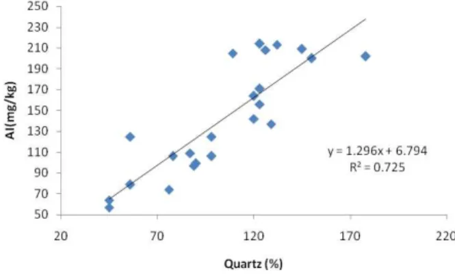
Fig. 4 illustrates the effects of Quartz on AI. Quartz is the hardest common mineral associated with coal [9]. The relationship between abrasive index (AI) and quartz in the coal is represented in Fig. 6 with R2 = 0.725.
Fig. 4. Effects of Quartz on abrasion index
The relationship between abrasive index (AI) and pyrite in the coal is represented in Fig. 5 with R2 = 0.776.
Fig. 5. Effects of pyrite on abrasion index
The correlation between abrasive index and ash percentage has been reported in literature [9], [18], [19]. A linear relationship was found between the two variables, with R2 = 0.805 as presented in Fig. 6. The ash yield essentially reflects the non-combustible residues of the different minerals associated with the coal.
Fig. 6. Effects of ash on abrasion index
High moisture content constituents of coals influenced AI of coal as illustrate in Fig. 7.
Fig. 7: Effects of H2O (moisture) abrasion index
IV. CONCLUSION
BPNN and GRNN techniques were employed to explore the nonlinear relationships between AI and four variables (Ash, Quartz, pyrite and moisture) on the abrasiveness characteristics of thermal coal. It was found that the obtained results of BPNN and GRNN predictions were in good agreement with the actual measurements, with coefficient of determination, R2 = 0.9003 for BPNN and R2 = 0.937 for GRNN. The good results indicated the NN techniques were capable of accurately modeling AI from thermal coal.
ACKNOWLEDGMENT
I would like to thank the Centre for Renewable Energy and Water for supporting this research.
REFERENCES
[1] J. Kabuba and A. Mulaba-Bafubiandi “Comparison of equilibrium study of binary system Co-Cu ions using adsorption isotherm models and Neural Network ”, in Proc. Conf. PSRC, Johannesburg, 2013, pp. 126-130.
[2] F. Lombard and C.J. Potgieter. Report on an Abrasive Index Investigation, Johannesburg, South Africa, 2008.
[3] C. Spero “Assessment and prediction of coal abrasiveness” Fuel, vol. 69, pp. 1168-1176, 1990.
[4] H.K Mishra, T.K. Chandra, R.P. Verma “Petrology of some Permian coals of India”, Int. J. Coal. Geol.., vol. 19, pp.47-71, 1990.
[5] E. Raask. Mineral Impurities in Coal Combustion-Behavior, Problems, and Remedial Measures, Hemisphere Publishing Corporation, Washington, 1995.
[6] M. Cumo, A. Naviglio “Thermal hydraulic design of components for
steam generation plants”, CRC Press, London, 1990.
[7] A.S Trimble, J.C. Hower “Studies of the relationship between coal petrology and grinding properties” Int. J. Coal Geol., vol. 54, pp. 253-260, 2003.
[8] D. Tickner and R.W. Maier. Design considerations for pulverized coal fired boilers combusting Illinois basin coals, Paper presented to Electric Power, April 5-7, Chicago, Illinois, USA, 2005.
[9] A.K. Bandopadhyay “A study on the abundance of quartz in thermal coals of India and its relation to abrasion index: Development of
predictive model for abrasion” Coal Geol., vol. 84, pp. 63-69, 2010.
[10] P. Li, Y. Xiong, D. Yu, X. Sun “Prediction of grindability with multivariable regression and neural network in Chinese coal” Fuel, vol. 84, pp. 2384-2388, 2005.
[11] A.H. Bagherieh, J.C. Hower, A.R. Bagherieh, E. Jorjani “Studies of
the relationship between petrography and grindability for Kentucky coals using artificial neural network” Int. J. Coal Geol., vol. 73, pp. 130-138, 2008.
[13] S.I.V.F.G. Sousa, M.C.M. Martins, Alvim-Ferraz and M.C. Pareira. Environ. Mod. Software, vol. 22, pp. 67-103, 2007.
[14] N.K. Kasabov. “Fuzzy systems and knowledge Engineering”,
Cambridge, Mass: MIT Press, 1998.
[15] G. Sun, S.J. Hoff, B.C. Zelle, M.A. Nelson. “Development and
comparison of Backpropagation and Generalized Regression Neural Models to predict Diurnal and Seasonal Gas and PM 10 concentrations an Emissions from swine Buildings”. Trans. ASABE, vol. 51, pp. 685-694.
[16] C.P. Snyman, M.C. Van Vaurer and J.M. Barnard. “Chemical &
physical characteristics of South African Coal and a suggested classification system”. Pretoria, National Institute of Coal Research, Coal Report no 8306, 1984.
[17] J.J. Wells, F. Wigley, D.G. Forster, W.H. Gibb, J. Williamson. “The
relationship between excluded mineral matter and the abrasion index of a coal”. Fuel, vol. 83, pp. 359-364.
[18] W.R. Livingston, K.L. Dugdale.”Modern coal mill design and
performance”. In. Proc. of the Conference and Exhibition
POWER-GEN, Asia, pp. 801-722, 1998.
[19] D.J. Foster, W.R. Livingston, J. Wells, W.H. Williamson, D. Gibb, D.
Bailey.” Particle impact erosion and abrasion wear-predictive methods
and remedial measures”. Report No COAL R241 DTI/Pub URN