Quantifying Changes of Soil Organic Carbon at Regional
Scale with a Biogeochemical Process Model
Liming Zhang1,2, Dongsheng Yu2*, Xuezheng Shi2, Shengxiang Xu2, Shihe Xing1*, Yongcong Zhao2
1College of Resource and Environment, Fujian Agriculture and Forestry University, Fuzhou, China,2State Key Laboratory of Soil and Sustainable Agriculture, Institute of Soil Science, Chinese Academy of Sciences, Nanjing, China
Abstract
Soil organic carbon (SOC) models were often applied to regions with high heterogeneity, but limited spatially differentiated soil information and simulation unit resolution. This study, carried out in the Tai-Lake region of China, defined the uncertainty derived from application of the DeNitrification-DeComposition (DNDC) biogeochemical model in an area with heterogeneous soil properties and different simulation units. Three different resolution soil attribute databases, a polygonal capture of mapping units at 1:50,000 (P5), a county-based database of 1:50,000 (C5) and county-based database of 1:14,000,000 (C14), were used as inputs for regional DNDC simulation. The P5 and C5 databases were combined with the 1:50,000 digital soil map, which is the most detailed soil database for the Tai-Lake region. The C14 database was combined with 1:14,000,000 digital soil map, which is a coarse database and is often used for modeling at a national or regional scale in China. The soil polygons of P5 database and county boundaries of C5 and C14 databases were used as basic simulation units. Results project that from 1982 to 2000, total SOC change in the top layer (0–30 cm) of the 2.3 M ha of paddy soil in the Tai-Lake region was+1.48 Tg C,23.99 Tg C and215.38 Tg C based on P5, C5 and C14 databases, respectively. With the total SOC change as modeled with P5 inputs as the baseline, which is the advantages of using detailed, polygon-based soil dataset, the relative deviation of C5 and C14 were 368% and 1126%, respectively. The comparison illustrates that DNDC simulation is strongly influenced by choice of fundamental geographic resolution as well as input soil attribute detail. The results also indicate that improving the framework of DNDC is essential in creating accurate models of the soil carbon cycle.
Citation:Zhang L, Yu D, Shi X, Xu S, Xing S, et al. (2014) Effects of Soil Data and Simulation Unit Resolution on Quantifying Changes of Soil Organic Carbon at Regional Scale with a Biogeochemical Process Model. PLoS ONE 9(2): e88622. doi:10.1371/journal.pone.0088622
Editor:Jose Luis Balcazar, Catalan Institute for Water Research (ICRA), Spain
ReceivedAugust 13, 2013;AcceptedJanuary 8, 2014;PublishedFebruary 11, 2014
Copyright:ß2014 Zhang et al. This is an open-access article distributed under the terms of the Creative Commons Attribution License, which permits unrestricted use, distribution, and reproduction in any medium, provided the original author and source are credited.
Funding:The work was funded by National Natural Science Foundation of China (No. 41001126), and the National Basic Research Program of China (973 Program) (2010CB950702). The funders had no role in study design, data collection and analysis, decision to publish, or preparation of the manuscript.
Competing Interests:The authors have declared that no competing interests exist.
* E-mail: [email protected] (DY); [email protected] (SX)
Introduction
An estimated 1500 Pg of C is held in the form of soil organic carbon (SOC), representing 2/3 of the global terrestrial organic carbon pool [1–3]. SOC plays a vital role in the global carbon cycle, where a slight alteration of the soil carbon pool can cause profound changes in atmospheric CO2 concentrations. Agro-ecosystems, accounting for 10% of the total terrestrial area, are one of the most sensitive terrestrial ecosystems subject to heavy human activity [3]. Increasing agricultural soil C sequestration is recognized as one strategy for achieving food security and improving soil quality.
Paddy soil is a major cultivated soil in China, and a unique type of anthropogenic soil recognized by Chinese Soil Taxonomy [3– 5]. The total area of paddy soils is 45.7 M ha, which accounts for 34% of the total cultivated land in China [6]. This area also accounts for 22% of the total waterlogged farming area worldwide and produces about 44% of all grain in China [4]. Therefore, accurate estimation of paddy soil SOC change in China is vitally important for a comprehensive understanding of SOC dynamics and agro-ecosystem sustainability.
Recently, scientists have applied modeling to estimate SOC change in cropping systems [7–14]. The DeNitrification-DeComposition
(DNDC) model, developed by Li et al. [15,16], is a process-based model focused on agrosystem carbon and nitrogen cycling and has been widely used for regional studies in the USA [17], China [11], India [18] and Europe [19]. Recently the DNDC model was determined to be one of the well performing models based on seven long-term experiments selected by the Global Change and Terrestrial Ecosystems Soil Organic Matter Network (GCTE SOMNET), which evaluated model perfor-mance using three different land uses, a range of climatic conditions within the temperate region, and different treatments [11,14].
conclusions that the DNDC model was capable of quantifying SOC change in the agroecosystems across the entire area of China.
To date, the county boundary was used as the basic simulation unit in most DNDC simulations conducted at regional scale [11,20]. As a result, these simulations are often subject to great uncertainties since the soil property data were averaged for the area, which greatly ignore the impacts of soil heterogeneity therein [18,22]. Moreover, many researchers used coarse soil attribute data obtained from the books such as Soil in China (Vol. 1–6) and 1: 14,000,000 soil maps at national or a regional scale in China [11,20]. However, studies have already pointed out that the effect of soil heterogeneity on SOC change estimation is a major source of uncertainty when using the DNDC model at the regional scale [18,22,23].
This study, which was carried out in the rice-dominated Tai-Lake Region of China, provides a chance to test the uncertainty of the DNDC model caused by different precisions of soil data and basic simulation unit. The goals of this study were to: (1) compare SOC changes modeled with different resolutions of soil databases and varied basic simulation units, (2) assess the uncertainty derived from these soil databases with different resolutions and basic simulation units, and (3) give some suggestions for improving the performance of the biogeochemical DNDC model applied at the regional scale.
Materials and Methods
Study area
The Tai-Lake region (118u509-121u549E, 29u569-32u169N), an area of intensive rice cultivation, is located in the middle and lower reaches of the Yangtze River paddy soil region of China. The region includes the entire Shanghai City administrative area and a part of Jiangsu and Zhejiang provinces, and covers a total area of 36,500 km2(Fig. 1) [4]. The Tai-Lake region mainly consists of plains formed on deltas with numerous rivers and lakes. The climate is warm and moist with abundant sunshine and a long growing season. Annual rainfall is 1,100–1,400 mm, with a mean temperature of 16uC, and average annual sunshine of 1,870– 2,225 hours. The frost-free period is over 230 days. The study area is one of the oldest agricultural regions in China, with a long history of rice cultivation spanning several centuries. Most
cropland in the region is managed as a rice and winter wheat rotation. Rice is planted in June and harvested in October and wheat is planted in November and harvested in May [24].
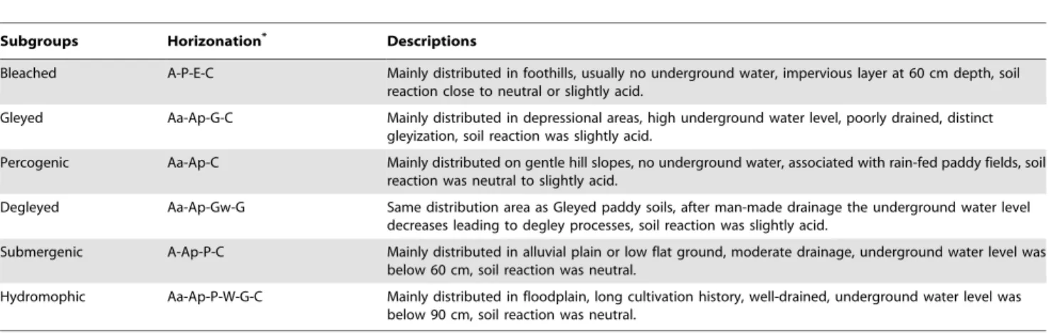
Approximately 66% of the total land area is covered with paddy soils [24]. Paddy soils in the Tai Lake area are derived mostly from loess, alluvium, and lacustrine deposits, and are classified into 6 soil subgroups according to the Genetic Soil Classification of China (GSCC) system which are represented in the 1:50,000 digital soil map (Table 1). As map scale decreased, the soil subgroups of submergenic, bleached, percogenic and degleyed on the 1:50,000 soil map was eliminated and emerged into the soil subgroups of degleyed and hydromorphic in the 1:14,000,000 soil map. Therefore, those were only two paddy soil subgroups of degleyed and hydromorphic in the 1:14,000,000 soil map. The GSCC nomenclature as well as the subgroup’s reference name in US Soil Taxonomy (ST) include; Hydromorphic (Typic Epia-quepts), Submergenic (Typic EndoaEpia-quepts), Bleached (Typic Epiaquepts), Gleyed (Typic Endoaquepts), Percogenic (Typic Epiaquepts), and Degleyed (Typic Endoaquepts) [25,26].
Description of the DNDC model
The DNDC model (Version 9.1) is a process-based soil biogeochemical research tool that was developed to estimate the impact of management strategies on the fate of nitrogen (N) and carbon (C) in agroecosystems. It integrates crop growth and soil biogeochemical processes on a daily time step and simulates N and C cycles in plant-soil systems.
The model contains six interacting sub-models which describe the generation, decomposition, and transformation of organic matter, and outputs the dynamic components of SOC and greenhouse gas fluxes. The six sub-models include: 1) a soil climate component which use soil physical properties, air temperature, and precipitation data to calculate soil temperature, moisture, and redox potential (Eh) profiles and soil water fluxes through time. The results of the calculation are then fed to the other sub-models; 2) a nitrification component; 3) a denitrification module, which calculates hourly denitrification rates and N2O, NO, and N2 production during periods when the soil Eh decreases due to rainfall, irrigation, flooding, or soil freezing; 4) simulation of SOC decomposition and CO2 production through soil microbial respiration; 5) a plant growth component, which calculates daily
root respiration, water, and N uptake by plants, and plant growth; and 6) a fermentation module, which calculates daily methane (CH4) production and oxidation. The DNDC model can simulate C and N biogeochemical cycles in paddy rice ecosystems, as the model has been modified by adding a series of anaerobic processes [15,16,22,23,27,28,29,30].
At present, the DNDC model has been utilized by scientists in many countries, for example, the model is applied to simulate the carbon cycle in paddy field in Italy, China and Germany, in wheat fields in Canada, and it has been used to simulate the dynamics of soil organic matter in a 100 year experimental field in Rothamsted Experimental Station in England [14,31]. At the international conference on global change in Asia-Pacific areas in 2000, the DNDC model was recommended as the primary method for SOC studies in the in the Asia-Pacific region [31].
Database development
A major challenge for using an ecosystem model at regional scale is to assemble adequate datasets required to initialize and run the model. We examined the influence of database choices by executing simulation runs with different input sets using individual or combinations of databases. The geographic resolution or fundamental simulation unit could be represented by any of three assessment unit format datasets, polygon-based database of 1:50,000 (P5), county-based database of 1:50,000 (C5), and county-based database of 1:14,000,000 (C14). The three soil datasets covered 37 counties in Tai-Lake region.
The polygon-based database of 1:50,000 (P5) was linked a digital soil map (1:50,000), the most detailed of the three databases, in the Tai-Lake region contains 52,034 paddy soil polygons (Table 2). The polygons were derived from 1,107 soil profiles extracted from the latest national soil map (1:50,000), the Second National Soil Survey of China in the 1980s-1990s, with attribute assignment using the Pedological Knowledge Based (PKB) method based on GSCC [32]. The 1:50,000 digital soil database consists of many soil attributes, such as soil name, horizon thickness, bulk density, organic carbon content, clay content, pH, etc.
Soil parameters in C5 were derived from the 1:50,000 digital soil map (Fig. 2 and Table 2). However the attributes for C14 were derived from different sources than C5, primarily the 1:14,000,000 national soil map [33,34] (Fig. 2). C14 was widely used when the DNDC model was applied to national or regional scale in China [11,20]. The C14 in the Tai-Lake region contained 8 polygons of paddy soils representing 49 paddy soil profiles, and was also compiled via the Pedological Knowledge Based (PKB) method based on GSCC [32].
The C5 and C14 were built from the default method developed for DNDC, in which the maximum and minimum values of soil texture, pH, bulk density, and organic carbon content were recorded for each county (Fig. 2). So, the DNDC modeling of C5 and C14 methods conducted have used counties as the basic simulation unit in the Tai-Lake region (Fig. 2). After regional runs with C5 and C14 database, the DNDC model produced two SOC
Table 2.Characteristics of different resolution soil attribute databases of paddy soils in GSCC in the Tai-Lake region, China.
Soil
database Map scale Source of soil maps Source of soil data
Basic map units
Number of soil profiles
Number of polygons
Simulation unit
P5 1:50,000 Soil Survey Office of County in Jiangsu Province, Zhejiang Province and Shanghai City
Soil Series of County in Jiangsu Province, Zhejiang Province and Shanghai City
Soil Species 1,107 52,034 polygon
C5 1:50,000 Soil Survey Office of County in Jiangsu Province, Zhejiang Province and Shanghai City
Soil Series of County in Jiangsu Province, Zhejiang Province and Shanghai City
Soil Species 1,107 52,034 county
C14 1:14,000,000 Institute of Soil Science, Chinese Academy of Sciences
Soil Series of China Subgroups 49 8 county
doi:10.1371/journal.pone.0088622.t002
Table 1.The subgroups of paddy soil in the Tai-Lake region, China.
Subgroups Horizonation* Descriptions
Bleached A-P-E-C Mainly distributed in foothills, usually no underground water, impervious layer at 60 cm depth, soil reaction close to neutral or slightly acid.
Gleyed Aa-Ap-G-C Mainly distributed in depressional areas, high underground water level, poorly drained, distinct gleyization, soil reaction was slightly acid.
Percogenic Aa-Ap-C Mainly distributed on gentle hill slopes, no underground water, associated with rain-fed paddy fields, soil reaction was neutral to slightly acid.
Degleyed Aa-Ap-Gw-G Same distribution area as Gleyed paddy soils, after man-made drainage the underground water level decreases leading to degley processes, soil reaction was slightly acid.
Submergenic A-Ap-P-C Mainly distributed in alluvial plain or low flat ground, moderate drainage, underground water level was below 60 cm, soil reaction was neutral.
Hydromophic Aa-Ap-P-W-G-C Mainly distributed in floodplain, long cultivation history, well-drained, underground water level was below 90 cm, soil reaction was neutral.
*According to GSCC (Genetic Soil Classification of China), Aa means arable layer, Ap plow pan, C undeveloped parent material, Ds fragmental deposit horizon, E bleached horizon, G gley horizon, Gw degley horizon, P percogenic horizon, W waterlogogenic horizon.
change (0–30 cm) resulting from two runs with the maximum and minimum soil values in each county. In this paper we present the mean results (average of maximum and minimum estimates) [11]. The DNDC modeling of P5 method conducted has used polygon as the basic simulation unit in the Tai-Lake region (Table 2). Therefore, the DNDC model runs with P5 database produced a single annual SOC change (0–30 cm) for each polygon. The total
SOC change of each county in the P5 was calculated by summing the SOC change of all polygons in a county. For a more complete description of P5 method see Zhang et al [35,36] and Xu et al [37].
For comparison in this study, both the polygon-based (P5) and county-based (C5 and C14) soil databases in the Tai-Lake region were run concurrently so the DNDC model could generalize regional SOC change from 1982 to 2000. The results simulated by DNDC with the two types of databases were compared to assess the advantages of using detailed, polygon-based 1:50,000 soil dataset (P5) [35,36,38,39].
In this study, the crop dataset included physiological data for summer rice and winter wheat in the Tai-Lake region. The crop parameters were obtained from thorough testing with that reflected the typical conditions of Tai-Lake region, which were founded on a wide range of information form Chinese literature published during the past decade and a publication of Gou et al [40,41].
Daily meteorological data (precipitation, maximum and mini-mum air temperature) for 1982–2000 from 13 weather stations across and near the Tai-Lake region were acquired from the National Meteorological Information Center, China Meteorolog-ical Administration (Fig. 3) [42]. Each county in the simulation was assigned to the nearest weather station [11,20,31].
The agricultural management dataset included sowing acreage, nitrogen fertilizer application rates, livestock, planting and harvest dates, and agricultural population at the county level from 1982 to 2000 in three resolution databases. The crop management practices of different counties were almost the same because the Tai-Lake region was a plain in topography. The main measures of farming management in the study area included: (1) fertilizer application: nitrogen synthetic fertilizer was applied for 6 times in the basal, tillering and heading stage for rice, and in the basal, jointing and heading stage for wheat; and organic manure (20% of
Figure 2. Description of C5 and C14 methods in the Tai-Lake region of China. doi:10.1371/journal.pone.0088622.g002
Figure 3. Geographical location of weather stations across or near the Tai-Lake region, China.
livestock wastes and 10% of human wastes) was applied twice as base fertilizer for rice and wheat at the rates calculated based on the local livestock numbers (866, 44, 95, and 23 kg C head21yr21 for cattle, sheep, swine and human, respectively); and N concentration in rainfall was 2.07 ppm; (2) crop residue manage-ment: 15% of aboveground crop residue was returned to the soil; (3) water management: one time of midseason and 5 time of shallow flooding (from June 17 to July 23, from July 28 to August 12, from August 24 to September 11, from September 18 to September 25, and from September 27 to October 2, respectively) were applied at summer rice; (4) tillage: twice at the 20 cm tilling depth for rice and 10 cm for wheat on the planting dates before 1990; and no-till applied for wheat after 1990; (5) growing period: rice is planted in June and harvested in October and wheat is planted in November and harvested in May; (6) optimum yield: rice is 7500 kg dry matter ha21and wheat is 3750 kg dry matter ha21[11,14,24,35,41,43]. All simulation methods within a certain county have the same feature input value such as crops, agricultural management, and climate, except soil feature [38,39].
Evaluation of simulation accuracy in three resolution databases
In order to evaluate the accuracy in three resolution databases, the simulated results of DNDC model were tested against measured data from paddy soils of the Tai-Lake region, which is the same area examined here.
From the perspective of previous studies, most dynamic models were only tested or validated with static long-term field-scale observations due to a lack of available soil data with temporal and spatial variation. Since these models have not yet been validated by regional scale data, uncertainty concerning their accuracy exists when they were applied to larger area dynamic SOC simulation [3].This study compared simulation results with the spatial distribution of SOC measurements from 1033 paddy soil sampling sites acquired in 2000, to validate and assess model performance in different simulation methods (P5, C5, and C14). The bias in the total difference between simulation and measurement were determined by calculating the correlation coefficient (r), the
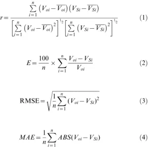
relative error (E), the mean absolute error (MAE) and the root mean square error (RMSE), as follows: [8,44].
r~
P
n
i~1
Voi{Voi
V
Si{VSi
P
n
i~1
Voi{Voi
2
1=2
P
n
i~1
VSi{VSi
2
1=2 ð1Þ
E~100 n |
X
n
i~1
Voi{VSi
Voi ð2Þ
RMSE~
ffiffiffiffiffiffiffiffiffiffiffiffiffiffiffiffiffiffiffiffiffiffiffiffiffiffiffiffiffiffiffiffiffiffi
1 n
X
n
i~1
(Voi{VSi)2
s
ð3Þ
MAE~1 n
X
n
i~1
ABS(Voi{VSi) ð4Þ
WhereVoiare the observed values,Voiis the mean of the observed data,VSi is the simulated value,VSi is the mean of the simulated value,Si[(P5,C5,C14), and n is the number in the sequence of the data pairs. If E is less than 5% or between 5% and 10%, the simulation is satisfactory or acceptable, respectively; otherwise, it is unacceptable [44]. The greater r value is and the smaller RMSE or MAE value is, the greater prediction accuracy is. Conversely, a lower r value and more elevated RMSE or MAE value, the lower prediction accuracy is.
Data comparison and analysis
SOC change as quantified by DNDC modeling with the P5 assessment unit data set are recognized as a benchmark for comparison with the results of the DNDC model runs with the other two assessment unit data sets as input. The P5 are thought
Figure 4. Spatial distribution of validation points and simulated SOC values from different simulation methods for the Tai-Lake region for 2000 (a: P5, b: C5, and c: C14).
theoretically to be more accurate than the C5 and C14 because of their relative greater detail and accuracy [35,36,38,39]. Relative variation of an index value (VIV, %) of C5 and C14 methods is calculated as the formula (1). The index values (IV) were quantified from the P5 data set (IVP5) and other data sets (IVCi) to support data set comparison [23,38,39].
VIV %ð Þ~ABS 100|ðIVP5 IVCiÞ=IVP5
ð5Þ
Where ABS is the absolute value function, IVP5is the total SOC change with P5, and IVCiis the total SOC change produced by C5 (or C14).
Previous results from the sensitivity tests of the DNDC model indicated that the spatial heterogeneity of soil properties (e.g. texture, SOC content, bulk density, and pH) are the major sources of uncertainty for simulating SOC changes under specific management conditions at regional scale [18,20,22,23]. In order to test the most sensitive soil properties factor, the correlation of soil properties and average annual SOC changes were determined by step-wise regression analysis by using SPSS statistical software [37,45]. The step-wise regression is useful in checking how entering each variable affects the overall regression model, which begins by entering the variable with the largest partial statistic and checking the importance of the coefficient of the variable [45,46]. This method keeps adding more variables, each time recalculating the coefficients. During the incorporation of a variable into the model, the partial statistic of the already entered variable changes and might cause it to be unimportant. The operation stops when the model has incorporated the variables with the most significant contribution and discarded the least significant ones [47].
Results and Discussion
Difference of simulation accuracy in three resolution databases
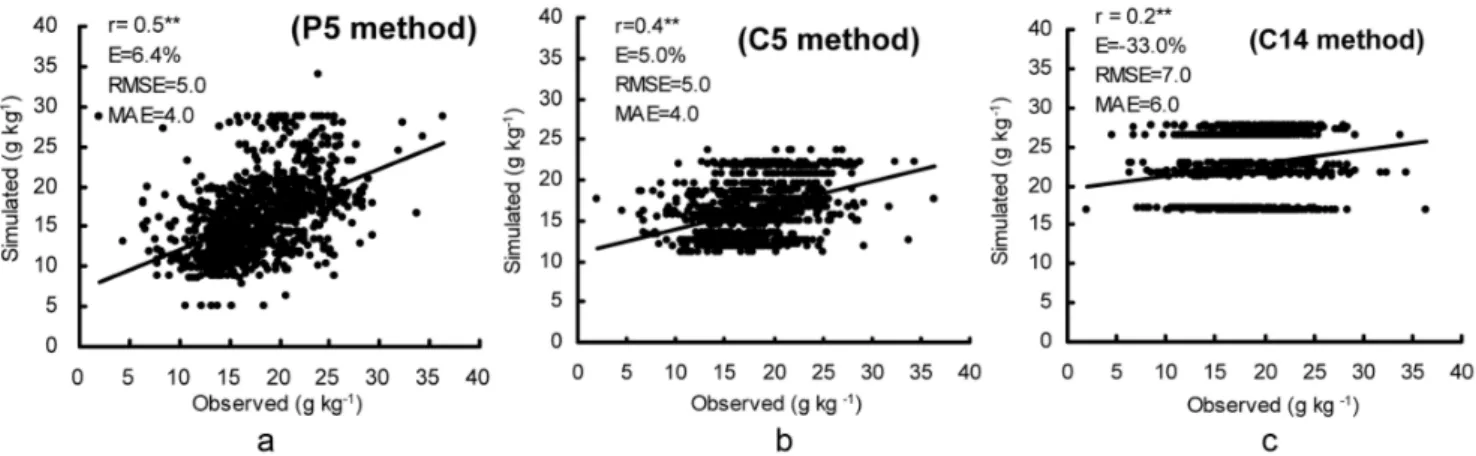
Three maps of average SOC content for paddy soils at surface layers (0–15 cm) in the study area in 2000 were constructed on the basis of simulated data in different simulation methods (P5, C5, and C14) (Fig. 4). Also, corresponding SOC validation points were constructed from measurements of the surface layer (0– 15 cm) of 1033 paddy soil samples taken in the study area in 2000. Fig. 4 demonstrates that the observed SOC in 2000 varied from 1.9 g kg21to 36 g kg21. By comparison, Fig. 4 also illustrates that
simulated SOC in 2000 varied from 5.1 g kg21to 34 g kg21in P5, from 11 g kg21to 24 g kg21in C5, and from 17 g kg21to 28 g kg21in C14; where 99.6%, 84.1% and 57.1% of simulated paddy soil samples in P5, C5 and C14 were within the ranges produced by the observed SOC data. Furthermore, the relative errors (E) of P5 and C5 were 6.4% and 5.0%, respectively; and within the range of 5%–10%, demonstrating that the DNDC model in P5 and C5 were acceptable for modeling SOC of paddy soils in the Tai-Lake region according to the evaluation criteria described earlier (Fig. 5a and b) [8,44]. Moreover, the small values of MAE (4.0 g kg21) and RMSE (5.0 g kg21) in P5 and C5 also indicated that the modeled results were encouragingly consistent with observations in the Tai-Lake region (Fig. 5a and b). However, the E, MAE and RMSE of C14 reached233%, 6.0 g kg21and 7.0 g kg21, respectively, suggesting that the simulated results of C14 were not suitable for simulating paddy soils in the Tai-Lake region (Fig. 5c).
Overall, though the values of E, MAE and RMSE between P5 and C5 had no significant differences, P5 was recognized better due to high correlation coefficient (0.5) and accurate simulation range (99.6%) (Fig. 5a and b). Furthermore, the simulation of P5 can differentiate the difference of paddy soil type within a county. Some studies showed that SOC content spatial variability was correlated with soil type spatial variability(Fig. 5a) [32,48,49]. Compared to the SOC validation of DNDC model in cropland by other scientists, accurate simulation of P5 (r = 0.50**; E = 6.4%; MAE = 4.0 g kg21; RMSE = 5.0 g kg21 and n = 1033) and C5 (r = 0.40**; E = 5.0%; MAE = 4.0 g kg21; RMSE = 5.0 g kg21and n = 1033) are higher than those of Liu et al [50] (r = 0.25–0.66 and n = 68), Liu et al [51] (E = 27.6% and n = 49), and Xu et al [52] (r = 0.22**; RMSE = 4.4 g kg21 and n = 243); and are almost similar to that of the Xu et al [52] (r = 0.52**; RMSE = 4.1 g kg21 and n = 1385). However, the SOC accurate simulation of DNDC model in P5, C5 and C14 are lower than those of Studdert et al [53] (r = 0.73**and n = 286) by using the RothC model and Yu et al [54] (r = 0.98** and n = 349) by using the Agro-C model. Therefore, the results mentioned above suggest that modification of the DNDC model is necessary to better simulate SOC change from cropping systems. With continued modification, DNDC model could become a powerful tool for estimating SOC change at regional and national scales.
Figure 5. Comparison between simulated and observed SOC values from different simulation methods of the Tai-Lake region for 2000 (a: P5, b: C5, and c: C14).
Variation of soil properties derived as input for DNDC modeling in three resolution databases in Tai-Lake region
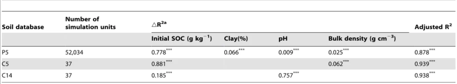
Results of the contribution of soil properties to the variability of average annual SOC change are given in Table 3. All variables (i.e., initial SOC content, pH, bulk density, and clay content) were included in the step-wise regression analysis. For the P5 and C5 resolution databases, initial SOC content accounted for 77.8%– 88.1% of the difference of average annual SOC change for paddy soils from 1982 to 2000, while other soil parameters only accounted for less than 6.6% of the difference. For the C14 resolution database, initial SOC content accounted for 18.5% of the difference of average annual SOC change for paddy soils from 1982 to 2000, and soil pH accounted for 75.7% of the difference. Therefore, it could be inferred that the differences in SOC change modeled with the three resolution databases were primarily due to the differences in initial SOC content and pH.
Table 4shows the initial SOC content (0–5 cm), clay content (0–10 cm), pH (0–10 cm), and bulk density (0–10 cm) derived as input for DNDC modeling, from P5, C5 and C14 for the Tai-Lake region. As for the entire Tai-Lake region, the average initial SOC values sourced from P5 was lower than that from C5 and C14. Another difference is that the average values of clay content and pH sourced from C14 were also higher than those from P5 and C5. The average bulk density sourced from C5 was higher than that from P5 and C14.
The differentiation of soil properties was also shown at the county scale in the Tai-Lake region (Table 4). The average values of initial SOC content and bulk density sourced from C5 for 24 counties were higher than those from P5; the other was that the average values of clay content for 24 counties and pH for 20 counties in C5 were lower than those from P5. Although the average clay content sourced from P5 for 25 counties was slightly lower than that from C14, but the average initial SOC content sourced from C14 for 34 counties was obviously higher than that of P5. According to statistics describing the 1:50,000 digital soil database of the Tai-Lake region, initial SOC content of six paddy soil subgroups, namely submergenic, bleached, percogenic, hydromorphic, degleyed and gleyed, were 10 g kg21, 10 g kg21, 11 g kg21, 15 g kg21, 19 g kg21, and 25 g kg21, respectively. As map scale decreased from 1:50,000 to 1:14,000,000, the submer-genic, bleached, percogenic and degleyed subgroups on the 1:50,000 digital soil map were eliminated and merged into the hydromorphic and degleyed subgroups in the 1:14,000,000 digital soil map [32,39]. The initial SOC content of the hydromorphic and gleyed subgroups in the 1:14,000,000 digital soil database were 17 g kg21 and 28 g kg21, respectively, which were higher than most paddy soil subgroups in the 1:50,000 digital soil
database. Therefore, the average initial SOC content of most counties in C14 was significantly higher than that from P5, while the average values of bulk density for 20 counties and pH for 24 counties in C14 was lower than those from P5. The results demonstrated that the soil properties (i.e., texture, SOC content, bulk density, and pH) in three resolution databases methods had large differences in the Tai-Lake region. Many studies have showed that SOC spatial variability is expressed by map delineations and map unit composition which varied with scales, resulting in the assignment of different soil properties at each scale of aggregation [32,48,49]. As such, an improper of soil map scales and simulation unit may lead to SOC estimation inaccuracy.
Variation of the average annual-, total SOC change modeled with the three resolution databases in Tai-Lake region
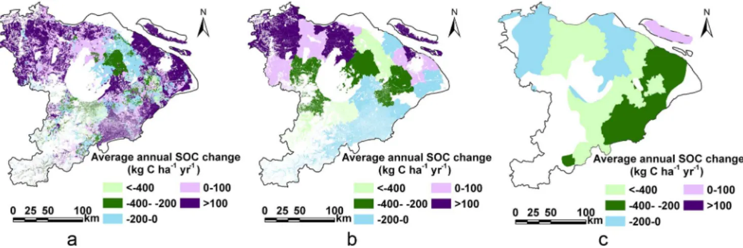
Similar trends can be observed in estimates of average annual-, total SOC change over the 19 year study period for three resolution databases decreased from P5 to C14 (Fig. 6). Simula-tion results demonstrate that total SOC change of P5 in the top layer (0–30 cm) of the 2.3 M ha of paddy rice fields in the Tai-Lake region was+1.48 Tg C from 1982 to 2000, with the annual SOC change ranging from -45 kg C ha21yr21to 92 kg C ha21 yr21(Fig. 6). From 1982 to 1988, the SOC change modeled with P5 inputs was almost negative with annual changes ranging from -3.2 kg C ha21 yr21 to -45 kg C ha21 yr21. According to agricultural statistical data, chemical fertilizer application rate ranged from 180 kg N ha21yr21to 350 kg N ha21yr21, which is a relatively low value. Low fertilizer application rates often result in reduced SOC sequestration [31,55]. From 1989 to 2000, rural economic development led to increased fertilizer application from 350 kg N ha21yr21to 400 kg N ha21yr21. Increasing fertilizer application results in enhanced crop production and residue accumulation, and the latter leads to an increase of SOC. Further, much of the region has been utilizing no-tillage practices in planting wheat since 1991, which contribute to reduced SOC decomposition [35].
Although three resolution databases within a certain county have the same feature input value such as crops, agricultural management, and climate; SOC balance of C5 (or C14) in the Tai-Lake region was almost negative with annual changes ranging from 86 kg C ha21yr21to -205 kg C ha21yr21(or -185 kg C ha21yr21to -693 kg C ha21yr21) from 1982 to 2000 (Fig. 6). The total SOC changes of C5 and C14 in the Tai-Lake region were23.99 Tg C and215.38 Tg C, respectively, from 1982 to 2000. With the total SOC change as modeled with P5 inputs as the baseline, the relative deviation of C5 and C14 were 368% and 1126%, respectively.
Table 3.Soil properties at three resolution soil attribute databases contributing to the variability of average annual SOC change in Tai-Lake region paddy soils from 1982 to 2000.
Soil database
Number of
simulation units gR
2a
Adjusted R2
Initial SOC (g kg21) Clay(%) pH Bulk density (g cm23)
P5 52,034 0.778*** 0.066*** 0.009*** 0.025*** 0.878***
C5 37 0.881*** 0.062*** 0.939***
C14 37 0.185*** 0.757*** 0.938***
***
significant at 0.001 probability levels, respectively.
As Table 3 illustrated, initial SOC content was the most sensitive parameter controlling SOC change among all soil factors in P5 and C5 [20,22]. The average initial SOC value of P5 and C5 were 15 g kg21 and 16 g kg21 for the entire Tai-Lake region, respectively. Furthermore, the average initial SOC content
sourced from P5 for 24 counties was lower than that from C5, while the average clay content sourced from P5 for 24 counties was also higher than that from C5. Many previous studies showed that soils with lower initial organic carbon and higher clay content tended to sequester C [20,22,35]. The high SOC sequestration Table 4.Statistics for soil properties derived as input for DNDC modeling in different counties, from P5, C5 and C14 for the Tai-Lake region.
County P5 C5 C14
SOC Clay BD pH SOC Clay BD pH SOC Clay BD pH
---WA--- Range Ave Range Ave Range Ave Range Ave Range Ave Range Ave Range Ave Range Ave
Zhangjiagang 14 28 1.22 7.7 10–17 14 5–32 19 1.16–1.33 1.25 7.4–8.0 7.7 12–21 17 24–31 28 1.19–1.23 1.21 6.0–7.4 6.7
Changshu 17 25 1.23 7.0 9–38 24 9–34 22 1.05–1.46 1.26 5.5–8.1 6.8 12–21 17 24–31 28 1.19–1.23 1.21 6.0–7.4 6.7
Taicnang 14 33 1.20 7.7 9–20 15 23–42 33 1.11–1.38 1.25 7.4–8.6 8.0 11–31 21 18–48 33 1.12–1.27 1.20 5.5–7.4 6.5
Kunshan 19 35 1.15 7.1 11–34 18 22–44 33 0.94–1.40 1.17 6.4–7.6 7.0 23–33 28 32–56 44 1.14–1.14 1.14 6.2–6.9 6.6
Wuxian 24 41 1.08 6.6 6–30 23 26–47 37 0.97–1.47 1.22 3.4–7.4 5.6 12–21 17 24–31 28 1.19–1.23 1.21 6.0–7.4 6.7
Wujiang 17 36 1.06 5.9 3–26 15 17–58 38 0.89–1.67 1.28 4.9–6.9 5.9 23–33 28 32–56 44 1.14–1.14 1.14 6.2–6.9 6.6
Wuxi 14 28 1.16 6.7 4–17 11 14–34 24 1.09–1.39 1.24 5.3–7.2 6.3 21–33 27 25–31 28 1.13–1.23 1.18 6.0–6.3 6.1
Jiangyin 13 13 1.28 6.2 6–17 12 8–25 17 0.99–1.54 1.27 5.4–8.0 6.7 21–33 27 25–31 28 1.13–1.23 1.18 6.0–6.3 6.1
Wujin 12 9 1.22 6.8 7–18 13 4–13 9 1.08–1.51 1.30 6.2–7.9 7.1 21–33 27 25–31 28 1.13–1.23 1.18 6.0–6.3 6.1
Jintan 10 9 1.32 6.8 7–14 11 4–13 9 1.17–1.58 1.38 5.5–7.6 6.6 12–21 17 24–31 28 1.19–1.23 1.21 6.0–7.4 6.7
Liyang 10 10 1.23 6.2 6–17 12 7–12 10 1.05–1.37 1.21 6.0–7.2 6.6 12–21 17 24–31 28 1.19–1.23 1.21 6.0–7.4 6.7
Yixing 13 27 1.17 6.0 3–30 17 10–53 32 1.11–1.58 1.35 4.4–8.5 6.5 21–33 27 25–31 28 1.13–1.23 1.18 6.0–6.3 6.1
Dantu 7 36 1.25 6.6 2–19 11 12–49 31 1.07–1.39 1.23 5.8–8.0 6.9 12–21 17 24–31 28 1.19–1.23 1.21 6.0–7.4 6.7
Jurong 10 30 1.23 5.4 6–13 10 15–38 27 1.10–1.29 1.20 5.1–7.4 6.3 12–21 17 24–31 28 1.19–1.23 1.21 6.0–7.4 6.7
Danyang 12 29 1.24 6.7 8–16 12 16–53 35 1.07–1.36 1.22 5.8–7.8 6.8 12–21 17 24–31 28 1.19–1.23 1.21 6.0–7.4 6.7
Jiaxing 19 34 1.19 6.5 10–26 18 20–56 38 0.98–1.34 1.16 5.8–7.6 6.7 23–33 28 32–56 44 1.14–1.14 1.14 6.2–6.9 6.6
Jiashan 21 39 1.23 6.2 15–27 21 22–44 33 1.03–1.34 1.19 5.7–7.0 6.4 23–33 28 32–56 44 1.14–1.14 1.14 6.2–6.9 6.6
Pinghu 15 35 1.10 6.6 9–24 17 22–43 33 0.92–1.48 1.20 6.3–7.2 6.8 11–31 21 18–48 33 1.12–1.27 1.20 5.5–7.4 6.5
Haiyan 17 40 1.17 6.7 7–25 16 22–52 37 0.92–1.51 1.22 5.7–7.3 6.5 11–31 21 18–48 33 1.12–1.27 1.20 5.5–7.4 6.5
Haining 14 36 1.19 6.6 7–24 16 19–52 36 0.92–1.51 1.22 6.0–7.5 6.8 11–31 21 18–48 33 1.12–1.27 1.20 5.5–7.4 6.5
Tongxiang 14 30 1.05 6.5 7–29 18 20–52 36 0.91–1.34 1.13 6.0–7.4 6.7 14–33 24 25–34 30 1.12–1.13 1.13 6.3–6.6 6.5
Huzhou 23 30 1.10 6.2 13–37 25 7–42 25 0.99–1.37 1.18 5.6–6.7 6.2 14–33 24 25–34 30 1.12–1.13 1.13 6.3–6.6 6.5
Changxing 17 31 1.14 5.8 6–31 19 9–47 28 0.84–1.53 1.19 3.6–7.1 5.4 14–33 24 25–34 30 1.12–1.13 1.13 6.3–6.6 6.5
Anji 18 22 1.16 6.0 12–34 23 12–42 27 0.84–1.44 1.14 5.4–6.7 6.1 14–33 24 24–35 30 1.12–1.13 1.13 6.3–6.6 6.5
Deqing 19 32 1.12 6.3 7–26 17 18–38 28 0.87–1.53 1.20 5.2–7.2 6.2 14–33 24 24–35 30 1.12–1.13 1.13 6.3–6.6 6.5
Yuhang 15 5 1.16 6.6 9–21 15 16–48 32 0.95–1.34 1.15 5.9–7.3 6.6 11–31 21 18–48 33 1.12–1.27 1.20 5.5–7.4 6.5
Linan 22 22 1.09 6.2 18–27 23 8–29 19 0.91–1.14 1.03 5.5–7.8 6.7 11–31 21 18–48 33 1.12–1.27 1.20 5.5–7.4 6.5
Minhang 13 26 1.18 7.6 10–18 14 17–46 32 1.11–1.30 1.21 6.4–8.0 7.2 11–31 21 18–48 33 1.12–1.27 1.20 5.5–7.4 6.5
Jiading 13 28 1.10 7.6 9–20 15 13–44 29 0.94–1.24 1.09 6.5–8.1 7.3 11–31 21 18–48 33 1.12–1.27 1.20 5.5–7.4 6.5
Chuangsha 12 29 1.15 7.6 9–20 15 17–36 27 1.06–1.33 1.20 7.3–8.0 7.7 11–31 21 18–48 33 1.12–1.27 1.20 5.5–7.4 6.5
Nanhui 16 31 1.18 7.4 13–22 18 8–35 22 1.11–1.21 1.16 6.5–8.1 7.3 11–31 21 18–48 33 1.12–1.27 1.20 5.5–7.4 6.5
Qingpu 21 27 1.15 7.1 7–33 20 11–36 24 0.94–1.53 1.24 5.6–8.3 7.0 23–33 28 32–56 44 1.14–1.14 1.14 6.2–6.9 6.6
Songjiang 23 26 1.20 6.8 10–33 22 8–37 23 1.03–1.47 1.25 5.6–8.1 6.9 23–33 28 32–56 44 1.14–1.14 1.14 6.2–6.9 6.6
Jinshan 20 29 1.22 7.0 11–37 24 18–36 27 1.11–1.47 1.29 4.6–8.3 6.5 11–31 21 18–48 33 1.12–1.27 1.20 5.5–7.4 6.5
Fengxian 15 25 1.20 7.4 12–18 15 19–39 29 1.11–1.49 1.30 6.9–8.1 7.5 11–31 21 18–48 33 1.12–1.27 1.20 5.5–7.4 6.5
Baoshan 11 23 1.21 7.9 9–19 14 8–44 26 1.11–1.28 1.20 7.2–8.2 7.7 11–31 21 18–48 33 1.12–1.27 1.20 5.5–7.4 6.5
Chongming 10 17 1.11 8.1 9–13 11 15–29 22 1.11–1.21 1.12 7.8–8.1 8.0 12–16 14 24–39 31 1.17–1.27 1.22 7.3–7.4 7.5
Tai-Lake region
15 26 1.18 6.7 2–38 16 4–58 27 0.84–1.54 1.23 3.4–8.3 6.7 11–33 22 18–56 32 1.12–1.27 1.18 5.5–7.4 6.5
WA = Weighted average of soil properties by the area of each polygon; SOC = Initial SOC content (g kg21
); Clay = Clay content (%); BD = Bulk Density (g cm23 ); Range = Range of maximum and minimum soil properties; Ave = Average of maximum and minimum soil properties.
rate (34 kg C ha21yr21) was thus associated with P5 (Fig. 7a). Conversely, the high SOC losses rate (-91 kg C ha21 yr21) was associated with C5 (Fig. 7b). The SOC losses rate (-349 kg C ha21yr21) in C14 was the highest in the three resolution databases (Fig. 7c). Table 3 demonstrates that pH and initial SOC content are the most sensitive parameters controlling SOC change among all soil factors in C14. The average initial SOC value (22 g kg21) of C14 was significantly higher than that of P5 (15 g kg21) and C5 (16 g kg21) for the entire Tai-Lake region. In addition, the average pH value of C14 for 34 counties was close to neutral (6.5–7.5), and the average initial SOC contents of C14 for 28 counties were higher than 20 g kg21. Some studies showed that soils with neutral pH value and higher organic carbon content were favorable for CO2 production by providing more substrates and better living environment for microbes [22,56].
The comparison illustrates that using different basic simulation units and soil data sources will produce different conclusions as to C sequestration or C liberation in the same study area. The implication is that more precise soil data and high resolution simulation units were necessary for better simulating regional scale SOC dynamics. The simulation outcome can be attributed to how the databases represent soil types and spatial heterogeneity, which is more precisely done with larger scale soil data and high resolution simulation units (e.g., 1:50,000 soil database).
Distribution of the average annual-, total SOC change modeled with the three resolution databases in different counties
The differentiation of the average annual-, total SOC change in P5, C5 and C14 was also shown at the county scale in the Tai-Lake region (Table 5 and Fig. 7). In the modeled domain, there were 26 counties that gained SOC and 11 counties that lost SOC from 1982 to 2000 in P5. The highest SOC sequestration rate of P5 were in Dantu, Jurong, Jiading and Baoshan counties which was higher than 200 kg C ha21yr21, due to the low initial SOC content (7.1 g kg21, 9.5 g kg21, 13 g kg21 and 11 g kg21, respectively). In addition, the clay content of P5 in Dantu and
Jurong counties were 36% and 30%, respectively. High clay content is associated with high SOC sequestration [22,57,58]. By contrast, the greatest SOC loss rate of P5 in the Huzhou, Songjiang, Linan and Wuxian county was more than 170 kg C ha21 yr21, due to the high initial SOC content (23 g kg21, 23 g kg21, 22 g kg21and 24 g kg21, respectively). Moreover, the clay content of P5 in Linan and Songjiang counties were only 22% and 26%, respectively. Low clay content is linked to high CO2 emissions [22].
However, under the same agricultural practice, there were only 14 counties that gained SOC and 23 counties that lost SOC from 1982 to 2000 in C5. The highest SOC sequestration rate of C5 were in Dantu, Jurong, Jintan, Chongming, and Baoshan counties which was higher than 150 kg C ha21yr21. The main reason was that the initial SOC content of C5 in Dantu, Jurong, Jintan, Chongming, and Baoshan counties were 11 g kg21, 10 g kg21, 11 g kg21, 11 g kg21and 14 g kg21, respectively; the other was that the average clay content of C5 in Dantu, Jurong, and Baoshan counties ranged from 26% to 31%. Some studies showed that low initial SOC value and high clay content were linked to low CO2 emissions [22,57,58]. In contrast, the greatest SOC loss rate of C5 in Jinshan, Changshu, Huzhou, Anji, and Kunshan county were more than 400 kg C ha21yr21, which possessed high initial SOC and low bulk density [22,35]. Compared with the P5 resolution database, the average annual-, total SOC change modeled with C5 for 28 counties was lower than that from P5. With the total SOC change as modeled with P5 inputs as the baseline, the relative deviations of counties in Jiangyin, Zhangjiagang and Kunshan were relatively high (.1000%). The relative deviations ranged from 50% to 250% in most counties. Only fifteen counties (Wuxian, Wujin, Jintan, Liyang, Dantu, Jurong, Huzhou, Yuhang, Linan, Minhang, Jiading, Chuangsha, Songjiang, Baoshan, and Chongming) had relatively low value of relative deviation (,100%). The SOC changes for the two resolution databases are almost in agreement with the soil feature across the 37 simulated counties (Table 4 and Table 5). The average initial SOC content sourced from C5 for 24 counties was higher than
Figure 6. Temporal distribution of average annual SOC change modeled with P5, C5 and C14 from 1982 to 2000 in the Tai-Lake region, China.
that from P5, and the average clay content sourced from C5 for 24 counties was also lower than that from P5. Some research showed that high initial SOC content and low clay content is favorable for C losses [22,57,58].
As can be seen from the Table 5, a big number of counties where the average annual-, total SOC change modeled with the C14 and P5 differed greatly. There was only one county that gained SOC from 1982 to 2000, while other 36 counties lost SOC in C14. The SOC losses of C14 ranged from 360 kg C ha21yr21 Table 5.Distribution of the average annual SOC change (kg C ha21yr21) and the total SOC change (Gg C) in different counties of the Tai-Lake region, China modeled with P5, C5 and C14 from 1982 to 2000.
County
Area
104ha P5 C5 C14
ASC TSC ASC TSC ASC TSC
WA Max Min AVE Max Min AVE Max Min AVE Max Min AVE
Zhangjiagang 2.54 2 1 138 250 44 66 224 21 57 2418 2181 27 2202 287
Changshu 7.55 264 292 246 21438 2596 353 22063 2855 92 2404 2156 132 2580 2224
Taicnang 6.14 43 50 241 2360 260 281 2420 270 192 2993 2400 224 21158 2467
Kunshan 7.57 38 55 252 21057 2402 362 21520 2579 275 2838 2456 2108 21205 2656
Wuxian 14.78 2172 2483 356 2876 2260 998 22458 2730 72 2403 2166 201 21132 2466
Wujiang 9.79 53 99 586 2717 265 1091 21333 2121 259 2792 2425 2110 21472 2791
Wuxi 9.77 49 91 478 2196 141 888 2364 262 2256 2958 2607 2476 21778 21127
Jiangyin 8.69 2 4 313 2101 106 517 2167 175 2262 2951 2606 2432 21569 21000
Wujin 14.85 91 256 248 257 96 701 2160 270 2274 2969 2621 2774 22734 21754
Jintan 7.10 146 197 245 81 163 331 110 220 136 2364 2114 184 2492 2154
Liyang 10.84 177 365 302 2115 94 623 2237 193 127 2386 2129 263 2796 2267
Yixing 10.34 147 289 514 21011 2248 1011 21987 2488 2262 2950 2606 2514 21867 21191
Dantu 5.07 371 357 615 2276 170 592 2266 163 141 2367 2113 136 2353 2109
Jurong 8.03 238 363 403 28 198 614 212 301 125 2374 2124 191 2570 2190
Danyang 9.58 47 85 416 2152 132 758 2276 241 130 2364 2117 237 2663 2213
Jiaxing 6.57 2124 2155 412 2523 255 514 2652 269 211 2752 2381 213 2938 2476
Jiashan 4.13 2103 281 110 2631 2260 87 2494 2204 248 2786 2417 238 2616 2327
Pinghu 4.81 127 116 349 2466 258 319 2425 253 274 2923 2324 250 2843 2296
Haiyan 2.74 41 21 489 2549 230 254 2285 216 279 2943 2332 145 2490 2173
Haining 3.92 151 113 483 2556 236 359 2413 227 274 2951 2338 204 2708 2252
Tongxiang 4.42 128 107 504 2634 265 424 2533 255 122 2846 2362 102 2711 2304
Huzhou 6.02 2309 2353 163 21184 2511 186 21354 2584 92 2915 2411 106 21046 2470
Changxing 5.62 42 45 422 2863 2221 450 2922 2236 71 2901 2415 76 2962 2443
Anji 4.18 266 252 178 21025 2423 141 2814 2336 58 2873 2408 46 2694 2324
Deqing 3.11 17 10 379 2684 2152 224 2404 290 77 2930 2426 46 2550 2252
Yuhang 5.27 291 292 344 2371 213 345 2372 213 120 21061 2456 120 21034 2457
Linan 3.06 2220 2128 7 2381 2187 4 2222 2109 218 2754 2268 127 2439 2156
Minhang 3.49 62 41 294 2239 28 195 2158 18 257 2974 2359 171 2645 2238
Jiading 4.29 238 194 387 2197 95 315 2161 77 281 2940 2329 229 2766 2268
Chuangsha 3.71 188 133 339 2295 22 239 2208 15 286 2925 2319 202 2653 2225
Nanhui 4.11 152 119 189 2279 245 148 2208 235 287 2939 2326 224 2734 2255
Qingpu 5.68 252 256 432 21042 2305 467 21125 2329 2 2756 2377 3 2816 2407
Songjiang 5.90 2287 2322 249 21010 2381 278 21131 2426 260 2816 2438 267 2914 2491
Jinshan 5.63 277 283 213 21481 2634 228 21585 2679 275 2945 2335 294 21011 2359
Fengxian 5.87 9 10 171 2270 249 191 2301 255 280 2944 2332 321 21053 2370
Baoshan 3.13 200 119 393 292 151 234 255 90 311 2876 2283 185 2522 2168
Chongming 3.73 195 138 283 47 165 201 34 117 165 2108 28 117 277 20
Tai-Lake region 232 34 1483 340 2521 291 14987 22297723994 46 2744 2349 2022 232790 215380
to 620 kg C ha21 yr21 in most counties. With the total SOC change as modeled with P5 inputs as the baseline, the relative deviations of counties in Zhangjiagang, Taicang, Kunshan, Wuxi, Jiangyin, Changxing, Deqing, and Fengxian were more than 1000%. Only five counties (Wuxian, Huzhou, Linan, Songjiang, and Chongming) in C14 had relatively low deviation (,100%). The main reasons were that the average pH value of C14 in most counties ranged from 6.5 to 7.5, which were closer to neutral than that from C5 and C14. Moreover, the average initial SOC contents of C14 in most counties were higher than 20 g kg21, which was also much higher than that from P5 or C5. Therefore, high SOC losses occurred in C14.
The modeled data at county scale in three simulation methods indicated the underestimation with the county-based database was related to its soil data source and simulation unit resolution, especially the coarse soil maps (1:14,000,000) that missed relatively small soil patches containing low or high soil properties (i.e., initial SOC content, pH, and clay content) which were sensitive to SOC change. This would also explain why the precision of soil database plays an important role in elevating the accuracy of modeled SOC change at regional scale.
Conclusions
Using different spatial information, process-based models integrated with GIS databases can play an important role in describing C biogeochemical cycles, such as targeting mitigation efforts to the most beneficial regions. However, SOC models have often been applied to regions with high heterogeneity but limited spatially differentiated soil information and simulated unit resolution.
Simulation results indicate that total SOC change from 1982 to 2000 in the top layer (0–30 cm) of the 2.3 M ha of paddy rice
fields in the Tai-Lake region was+1.48 Tg C for P5. However, discrepancies in the results existed among the three databases, because different soil data and basic simulation units were used. The total SOC changes in the Tai-Lake region were -3.99 Tg C and -15.38 Tg C for C5 (or C14), respectively, from 1982 to 2000. With the total SOC change as modeled with P5 inputs as the baseline, the relative deviation of C5 was lower than C14 due to the more precise soil data. In contrast, the relative deviation of C14 was higher than other databases due to using coarser soil data and low-resolution simulation units. In addition, with the same basic simulation unit, average annual-, total SOC change between C5 and C14 for the Tai-Lake region also had a large discrepancy due to the use of different soil data. The comparison demonstrated that the most sensitive factors (e.g., initial SOC content and pH) for modeling SOC dynamics should be given a high priority during the input data acquisition as they contribute dispropor-tionately to the uncertainties produced during the upscaling process [20]. The results also indicate that improving the performance of the biogeochemical DNDC model is essential in creating accurate models of the soil carbon cycle.
Acknowledgments
We gratefully acknowledge support for this research from the National Natural Science Foundation of China (No. 41001126), and the National Basic Research Program of China (973 Program) (2010CB950702). Sincere thank is also given to Professor Changsheng Li (University of New Hampshire, USA) for his useful advice on DNDC model.
Author Contributions
Conceived and designed the experiments: DSY XZS SHX. Performed the experiments: LMZ SXX. Analyzed the data: LMZ SXX. Contributed reagents/materials/analysis tools: SXX YCZ. Wrote the paper: LMZ.
References
1. Eswaran H, Berg EVD, Reich P (1993) Organic carbon in soil of the world. Soil Science Society of America Journal 57:192–194.
2. Lal R (2006) World soils and greenhouse effect: An overview, in soils and global change. Encyclopedia of Soil Science. doi:10.1081/E-ESS-120042696. 3. Shi XZ, Yang RW, Weindorf DC, Wang HJ, Yu DS, et al. (2010) Simulation of
organic carbon dynamics at regional scale for paddy soils in China. Climatic Change 102:579–593.
4. Li QK (1992) Paddy soil of China. Beijing: Science Press. 514 p.
5. Gong ZT (1999) Chinese soil taxonomic classification. Beijing: Science Press. 5– 215 p.
6. Liu QH, Shi XZ, Weindorf DC, Yu DS, Zhao YC, et al. (2006) Soil organic carbon storage of paddy soils in China using the 1:1,000,000 soil database and their implications for C sequestration. Global Biogeochemical Cycles 20:GB3024. doi:10.1029/2006GB002731.
7. Jenkinson DS, Rayner JH (1977) The turnover of soil organic matter in some of Rothamsted classical experiments. Soil Science 125:298–305.
8. Smith P, Smith JU, Powlson DS, Arah JRM, Chertov OG, et al. (1997) A comparison of the performance of nine soil organic matter models using datasets from seven long term experiments. Geoderma 81:153–225.
Figure 7. Spatial distribution of average annual SOC change modeled with P5, C5 and C14 in the Tai-Lake region, China (a: P5, b: c5, and c:C14).
9. Ardo¨ J, Olsson L (2003) Assessment of soil organic carbon in semi-arid Sudan using GIS and the CENTURY model. Journal of Arid Environments 54:633– 651.
10. Shirato Y (2005) Testing the suitability of the DNDC model for simulating long-term soil organic carbon dynamics in Japanese paddy soils. Soil Science and Plant Nutrition 51(2):183–192.
11. Tang HJ, Qiu JJ, van Ranst E, Li CS (2006) Estimations of soil organic carbon storage in cropland of China based on DNDC model. Geoderma 134:200–206. 12. Cerri CEP, Easter M, Paustian K, Killian K, Coleman K, et al. (2007) Predicted soil organic carbon stocks and changed in the Brazilian Amazon between 2000 and 2030. Agriculture, Ecosystems and Environment 122:58–72.
13. Huang Y, Yu YQ, Zhang W, Sun WJ, Liu SL, et al. (2009) Agro-C: A biogeophysical model for simulating the carbon budget of agroecosystems. Agricultural and Forest Meteorology 149:106–129.
14. Tang HJ, Qiu JJ, Wang LG, Li H, Li CS, et al. (2010) Modeling soil organic carbon storage and its dynamics in croplands of China. Agricultural Sciences in China 9(5):704–712.
15. Li CS, Frolking S, Frolking TA (1992) A model of nitrous oxide evolution from soil driven by rainfall events: I. Model structure and sensitivity. Journal of Geophysical Research 97:9759–9776.
16. Li CS, Frolking S, Frolking TA (1992) A model of nitrous oxide evolution from soil driven by rainfall events:II. Model applications. Journal of Geophysical Research 97:9777–9783.
17. Tonitto C, David MB, Li CS, Drinkwater LE (2007) Application of the DNDC model to tile-drained Illinois agroecosystems: Model comparison of conventional and diversified rotations. Nutrient Cycling in Agroecosystems 78 (1):65–81. 18. Pathak H, Li CS, Wassmann H (2005) Greenhouse gas emissions from Indian
rice fields: calibration and upscaling using the DNDC model. Biogeoscience 2:113–123.
19. Neufeldt H, Scha¨fe M, Angenendt E, Li CS, Kaltschmitt M, et al. (2006) Disaggregated greenhouse gas emission inventories from agriculture via a coupled economic-ecosystem model. Agriculture, Ecosystems and Environment 112:233–240.
20. Zhang F, Li CS, Wang Z, Wu HB (2006) Modeling impacts of management alternatives on soil carbon storage of farmland in Northwest China. Biogeosciences 3:451–466.
21. Wang LG, Qiu JJ, Tang HJ, Li CS, van Ranst E (2008) Modelling soil organic carbon dynamics in the major agricultural regions of China. Geoderma 147:47– 55.
22. Li CS, Mosier A, Wassmann R, Cai ZC, Zheng XH, et al. (2004) Modeling greenhouse gas emissions from rice-based production systems: Sensitivity and upscaling. Global Biogeochemical Cycles 18:GB1043. doi:10.1029/2003 GB002045.
23. Cai ZC, Sawamoto T, Li CS, Kang GD, Boonjawat J, et al. (2003) Field validation of the DNDC model for greenhouse gas emissions in East Asian cropping systems. Global Biogeochemical Cycles 17 (4): GB1107, doi:10.1029/ 2003 GB002046.
24. Xu Q, Lu YC, Liu YC, Zhu HG (1980) Paddy soil of Tai-Lake region in China. Shanghai: Science Press.
25. Shi XZ, Yu DS, Warner ED, Sun WX, Petersen GW, et al. (2006) Cross-reference system for translating between genetic soil classification of China and Soil Taxonomy. Soil Science Society of America Journal 70:78–83. 26. Soil Survey Staff in USDA (2010) Keys to Soil Taxonomy (11th Edition).
Washington: USDA-Natural Resources Conservation Service.
27. Li CS, Frolking S, Harriss R (1994) Modeling carbon biogeochemistry in agricultural soils. Global Biogeochemical Cycles 8 (3):237–254.
28. Li CS, Narayanan V, Harriss R (1996) Model estimates of nitrous oxide emissions from agricultural lands in the United States. Global Biogeochemical Cycles 10 (2):297–306.
29. Li CS, Qiu JJ, Frolking S, Xiao XM, Salas W, et al. (2002) Reduced methane emissions from large-scale changes in water management in China’s rice paddies during 1980–2000. Geophysical Research Letters 29 (20):1972, doi:10.1029/ 2002GL01 5370.
30. Li CS (2007) Quantifying greenhouse gas emissions from soils: Scientific basis and modeling approach. Soil Science and Plant Nutrition 53 (4):344-352. 31. Qiu JJ, Wang LG, Tang HJ, Li H, Li CS (2005) Studies on the situation of soil
organic carbon storage in croplands in northeast of China. Agricultural Sciences in China 37 (8):1166–1171.
32. Zhao YC, Shi XZ, Weindorf DC, Yu DS, Sun WX, et al. (2006) Map scale effects on soil organic carbon stock estimation in north China. Soil Science Society of America Journal 70:1377–1386.
33. Institute of Soil Science (1986) The soil atlas of China. Beijing: Institute of Soil Science, Academia Sinica, Cartographic Publishing House.
34. National Soil Survey Office of China (1993–1997) Soils in China (Vol. 1–6). Beijing: Agricultural Publishing House.
35. Zhang LM, Yu DS, Shi XZ, Xu SX, Wang SH, et al. (2012) Simulation soil organic carbon change in China’s Tai-Lake paddy soils. Soil and Tillage Research 121:1–9.
36. Zhang LM, Yu DS, Shi XZ, Xu SX, Weindorf DC, et al. (2009) Quantifying methane emissions from rice fields in the Taihu region, China by coupling a detailed soil database with biogeochemical model. Biogeosciences 6:739–749. 37. Xu SX, Zhao YC, Shi XZ, Yu DS, Li CS, et al. (2013) Map scale effects of soil
databases on modeling organic carbon dynamics for paddy soils of China. Catena 104:67–76.
38. Yu DS, Yang H, Shi XZ, Warner ED, Zhang LM, et al. (2011) Effects of soil spatial resolution on quantifying CH4and N2O emissions from rice fields in the Tai Lake region of China by DNDC model. Global Biogeochemical Cycles 25:GB2004. doi:10.1029/2010GB003825.
39. Yu DS, Zhang LM, Shi XZ, Warner ED, Zhang ZQ, et al. (2013) Soil assessment unit scale affects quantifying CH4emissions from rice fields. Soil Science Society of America Journal 77:664–672.
40. Li CS (2007) Quantifying soil organic carbon sequestration potential with modeling approach. In: Tang HJ, Van Ranst E, Qiu JJ (Eds.) Simulation of soil organic carbon storage and changes in agricultural cropland in China and its impact on food security. Beijing: China Meteorological Press. 1–14 p. 41. Gou J, Zheng XH, Wang MX, Li CS (1999) Modeling N2O emissions from
agriculture fields in Southeast China. Advances in Atmospheric Sciences 16 (4):581–592.
42. China Meteorological Administration (2011) China meteorological data daily value. China Meteorological Data Sharing Service System, Beijing, China. http://cdc.cma.gov.cn/index.jsp.
43. Lu RK, Shi TJ (1982) Agricultural chemical manual. Beijing:China Science Press. 142 p.
44. Whitmore AP, Klein-Gunnewiek H, Crocker GJ, Klir J, Ko¨rschens M, et al. (1997) Simulating trends in soil organic carbon in long-term experiments using the Verberne/MOTOR model. Geoderma 81:137–151.
45. Admassu Y, Shakoor A, Wells N (2012) Evaluating selected factors affecting the depth of undercutting in rocks subject to differential weathering. Engineering Geology 124:1–11.
46. Leech NL, Barret KKC, Morgan G (2008) SPSS for intermediate statistics. New York: Lawrence Erlbaum Associates. 270 p.
47. Dielman TE (2001) Applied regression analysis for business and economics. California: Duxbury Thomson Learning. 647 p.
48. Arnold RW (1995) Role of soil survey in obtaining a global carbon budget. In: Lal R, Kimble J, Levine E, Stewart BA (Eds.) Advances in Soil Science: Soils and Global Change. Boca Raton, FL: CRC Press. 57–263 p.
49. Zhong B, Xu YJ (2011) Scale effects of geographical soil datasets on soil carbon estimation in Louisiana, USA: a comparison of STATSGO and SSURGO. Pedosphere 21 (4):491–501.
50. Liu YH, Yu ZR, Chen J, Zhang FR, Reiner D, et al. (2006) Changes of soil organic carbon in an intensively cultivated agricultural region: A denitrification-decomposition (DNDC) modelling approach. Science of the Total Environment 372:203–214.
51. Liu Q, Sun B, Jie XL, Li ZP (2009) The spatial-temporal dynamic change and simulation of county-scale paddy soil organic carbon red soil hilly region. Acta pedologica sinica 46 (6):1059–1067.
52. Xu SX, Shi XZ, Zhao YC, Yu DS, Wang SH, et al. (2012) Spatially explicit simulation of soil organic carbon dynamics in China’s paddy soils. Catena 92:113–121.
53. Studdert GA, Monterubbianesi GM, Domı´nguez GF (2011) Use of RothC to simulate changes of organic carbon stock in the arable layer of a Mollisol of the southeastern Pampas under continuous cropping. Soil and Tillage Research 117:191–200.
54. Yu YQ, Huang Y, Zhang W (2012) Modeling soil organic carbon change in croplands of China, 1980-2009. Global and Planetary Change 82–83:115–128. 55. Wu TY, Schoenau JJ, Li FM, Qian PY, Malhi SS (2004) Influence of cultivation and fertilization on total organic carbon and carbon fractions in soils from the Loess Plateau of China. Soil and Tillage Research 77:59–68.
56. Pacey JG, DeGier JP (1986) The factors influencing landfill gas production. In: Energy from landfill gas. Proceeding of a conference jointly sponsored by the United Kingdom Department of Energy and the United States Department of Energy (October 1986). 51–59 p.
57. Burke IC, Lauenroth WK, Conffin DP (1995) Soil organic matter recovery in semiarid grassland: implications for the conservation reserve program. Ecological Monographs 5:793–801.