MODELING PRECIPITATION OF SHORT DURATION BY MEANS OF THE MODIFIED
BARTLETT-LEWIS RECTANGULAR PULSE MODEL
ÁLVARO JOSÉ BACK
1, EDISON UGGIONI
2AND HAMILTON JUSTINO VIEIRA
3 1Empresa de Pesquisa Agropecuária e Extensão Rural de Santa Catarina (Epagri), Urussanga, SC;
Universidade do Extremo Sul Catarinense (Unesc), Criciúma,SC, Brasil.
2
Universidade do Extremo Sul Catarinense (Unesc), Criciúma, SC, Brasil,.
3
Empresa de Pesquisa Agropecuária e Extensão Rural de Santa Catarina (Epagri), Florianópolis,SC, Brasil.
[email protected], [email protected], [email protected]
Received April 2009 - Accepted March 2011
ABSTRACTThe objective of this work was to evaluate the mathematical modeling of rainfall of duration less than one hour using the modiied Bartlett-Lewis model with six parameters. The data used were for the period October 1980 to December 2007, from recording rain gauges (pluviographs) at the meteorological station of Epagri, Urussanga, south of Santa Catarina (latitude 28.31° S, longitude 48.19 ° W). Based on simulations of series with 100 years of data it can be concluded that: the adjustment of the parameters of the modiied Bartlett-Lewis model enables the simulation of rain at intervals as small as 5 minutes of duration, preserving the statistical properties of precipitation over various intervals of aggregation in time. In general there was a tendency toward overestimation of the probability of dry periods and underestimation of the covariance for intervals of 24 hours, especially in summer. The total annual rainfall simulated for all time intervals examined remains within the conidence interval of 95%. Keywords: Rainfall, simulation, hydrology.
RESUMO: MODELAGEM DA PRECIPITAÇÃO DE CURTA DURAÇÃO POR MEIO DO MODELO
DE PULSOS RETANGULARES DE BARTLETT-LEWIS MODIFICADO
Este trabalho teve como objetivo avaliar a modelagem matemática da precipitação pluviométrica de duração inferior a uma hora por meio do modelo de Bartlett-Lewis modiicado com seis parâmetros. Foi utilizada a série de dados pluviográicos do período de outubro de 1980 a dezembro de 2007 da estação meteorológica da Epagri, Urussanga, Sul de Santa Catarina (latitude 28,31º S, longitude 48,19º W). Com base nas simulações de séries com 100 anos de dados pode-se concluir que: o ajuste dos parâmetros do modelo de Bartlett-Lewis modiicado possibilita a simulação de chuvas com intervalos de duração de até 5 minutos preservando as propriedades estatísticas da precipitação em vários níveis de agregação temporal. De forma geral observou-se a tendência de superestimativa da probabilidade dos períodos serem secos e subestimativa da covariância para intervalos de 24 horas, principalmente no verão e que os totais anuais de chuva simulada para todos os intervalos de duração analisados permanecem dentro do intervalo de coniança de 95%.
Palavras-chave: precipitação, simulação, hidrologia
1. INTRODUCTION
Rainfall is one of the elements of climate that have high temporal and spatial variability, and its occurrence in excess or deicit usually causes damage to agricultural production as well as disruptions for the general population. To determine the scale of the engineering projects to be carried out to overcome the problems of excess or insuficient rainfall, values of rainfall
and their associated risk of occurrence, called design values, are used. These values are obtained through analysis of long series of observed data, and therefore can only be obtained in locations with long historical records of precipitation.
al. (2008) and Back (2009) reported the dificulty of obtaining long series of rainfall data, primarily from rain gauge records. Cecilio and Pruski (2003) also emphasize that the methodology for determining intensity-duration-frequency relationships for rainfall requires extensive work in tabulation, analysis and interpretation of a large number of pluviograms. According to Genneville and Boock (1983) and Golden Neto et al. (2005), the use of reduced time series increases the likelihood of obtaining values that are biased toward particular regions.
The use of mathematical modeling for the simulation of rain can be a tool for assessing these problems because it has the advantage of being able to obtain long series of data without gaps, making it possible to simulate the functioning of hydrologic systems in different scenarios. Various widely-used models exist for the simulation of daily rainfall; but little work has been presented on the testing of models of rainfall of shorter duration. Mello et al. (2009) applied precipitation modeling to the estimation of monthly and annual precipitation in the state of Minas Gerais. Lima et al. (2005) evaluated the Cligen model in the simulation of daily and monthly rainfall in southern Portugal. Oliveira et al. (2005), Cecílio and Pruski (2003), Back (2009) comment on the use of precipitation series of short duration for the determination of intensity-duration-frequency relations, of wide application in the planning of hydraulic projects. The use of Markov chains is prominent in models of daily precipitation (Andrade Junior et al. 2001; Oliveira et al. 2005). According to Damé et al. (2007) an important consideration to be made is that the stochastic models with Markovian structure do not take into consideration the clustering of rain cells, which is a characteristic clearly exhibited by precipitation, as much at a spatial as at a temporal level; because of this they are considered limited when dealing with the modeling of precipitation maxima. This characteristic of the precipitation process makes necessary the extension of the analysis to statistical moments of the second order - variance, covariance and the autocorrelation coeficient - as a means of obtaining a closer it to the physical phenomenon involved.
Among the diverse rain simulation models based on the theory of point processes are the models with rectangular jumps, based on the clustering of rain cells. According to Rodriguez-Iturbe (1987) these models represent the rainfall phenomenon as a simple series of steps in time. This characteristic makes these models useful tools in the majority of hydrological studies, serving to evaluate the production of surface runoff and predictions of discharge rates, among other applications. The models of point processes for precipitation, such as the rectangular pulse model of Nayman-Scott and the rectangular pulse models described by Rodriguez-Iturbe represent a great advance in the modeling of precipitation. These models consider rain events to be formed from cells, basic units of precipitation,
whose distribution in time follows a deined stochastic process. The models were applied to precipitation data from Denver by Rodriguez-Iturbe et al. (1987), who observed that they are capable of preserving the main statistical characteristics of the precipitation, including extreme values, in periods of 1 hour up to 24 hours, although they were incapable of preserving the proportion of dry periods over levels of aggregation above 1 hour. Rodriguez-Iturbe (1988) modiied the rectangular pulse model of Bartlett-Lewis, allowing the parameter for the exponential distribution of the duration of the cell to vary from shower to shower according to a gamma distribution. With this modiication, the model was also capable of reproducing the proportion of dry periods over various intervals of time. The modiied model has six parameters and is called the modiied Bartlett-Lewis model. Entekhabi et al. (1989) and Cowpertwait et al. (1996), Khaliq and Cunnane (1996) studied different forms of adjustment of the parameters for simulation of hourly precipitation. Back et al. (1999) applied the rectangular pulse model in the generation of rain series in hourly intervals. Damé (2006), having rain gauge data from 1982 to 1988 from the city of Pelotas in Rio Grande do Sul for his studies on the de-aggregation of daily precipitation amounts into estimates of curves of intensity-duration-frequency, also utilized the modiied rectangular pulse rainfall simulation model of Bartlett-Lewis to verify by use of this model if the simulated rainfall preserved the statistical characteristics of the precipitation process.
The objective of this work is to evaluate the utilization of the modiied rectangular pulse model of Bartlett-Lewis in series of precipitation with duration of less than 1 hour.
2. MATERIAL AND METHODS
always registered as errors in the data. Along with the digitized archives, secondary archives were also generated, with data discretized in intervals of 1 h, 30 min, 15 min, 10 min and 5 min. For the simulation of the series of hourly rainfall the stochastic model adopted was the modiied Bartlett-Lewis rectangular pulse model with 6 parameters. The resolution of the hourly data was of the order of 0.1 mm, and whenever the precipitation observed during an interval of time was less than this, the interval was deined as dry. To consider the seasonal variance of the values of precipitation, the parameters of the model are estimated separately for each month.
The procedure adopted for the adjustment of the parameters was that described by Entekhabi et al.(1989) and by Cowpertwait et al. (1996), which consists of minimizing the sum of the squares of the deviations between the values observed and the values estimated by the model. In this scheme the residuals are normalized by the respective historical values. Thus considering
fi fi(l, a, u, k, f, mx) as being a function of the model
and f as being a sample value taken from a historical series of values, and assuming m functions, the estimate of the parameters
can be made minimizing the following sum of squares:
in which: fi =analytic function deined by the model;
fo = corresponding value estimated from the observed data;
m = number of functions considered.
In order to minimize the summation of the function (1), the “Solver” command of the Excel spreadsheet (Lapponi, 2005) was utilized. This program employs a quasi-Newtonian method for the minimization of values.
The functions utilized represented the one-hour mean, the variance, the autocorrelation coeficient with lag 1 and the proportion of dry periods for the intervals 1, 6, 12 and 24 hours.
The mean of the observed values for each interval of the duration was estimated by the function:
where: mk(h) = observed mean for the time interval of h hours (mm);
k = index of calendar month (k=1 for January, 2 for February, etc...);
= value of total precipitation of the j-th interval of the year i for month k;
= total number of time intervals of h hours in month k; n = number of years of data.
The variance of the precipitation will be estimated by the function:
≡
(1)
(
)
2 11 /
m
i o
i
S f f
= =
∑
−( )
( ) ( ){ }
( ) , , 1 1 / h k n n h hk i j k k
i j
h Y n n
m
= =
=
∑∑
(2)
( ) , ,h i j k
Y
( )h k
n
in which: g(h) = variance observed over the time interval (mm-2).
The autocovariance with lag 1 is estimated by the function:
in which: gk(h,1) = autocovariance with lag 1 (mm-2).
The autocorrelation coeficient with lag 1 is given by the relation between the autocovariance with lag 1 and the variance, that is:
in which: r(h,1) = autocorrelation coeficient with lag 1. The proportion of dry intervals is estimated as the ratio between the number of dry intervals of h hours and the total number of intervals of h hours in month k, that is:
in which : fd is the proportion of intervals of h hours duration without rain and nd is the number of these intervals observed.
The analytic form of the model of rectangular pulses of Bartlett-Lewis, which deines the mean of the precipitation values in an interval of h hours is given by:
In which: : E(Yh) =mean precipitation in an interval
of h hours (mm);
l, u, mx, a, f, K are the parameters of the model;
h = interval of time (h).
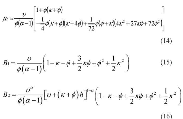
The variance of the precipitation is defined by the following expression:
in which: Var[Yh] = variance of the values of precipitation in
the interval of h hours (mm2);
(3)
( )
( )( )
{
}
( ) ( ) 2 , , 1 1 h k n n hi j k k
i j k h k Y h h n n m
g = =
− =
∑∑
( )
( )( )
{
}
( ) ( )( )
{
}
( ) 1, , , 1,
1 1 ,1 ( 1) h k n n h h
i j k k i j k k
i j
k h
k
Y h Y h
h n n m m g − + = = − − = −
∑ ∑
(4) (5)( )
,1 k( )
( )
,1 k h h h g r g =fd(h) = n (6)d(h)/ ( )h k
n
(7)
( )
h 1x c ih E Y l um m
a
= −
mc = 1 + (8)K/f;
(9)
(
)
2 3(
)
31
2 3
h i
Y Aa hu −a u −a u h −a
= − − + +
(
)
2 3(
)
32
2A a 3 f uh −a u −a u fh −a
− − − + + var
(
)(
)(
)
( )
2 2 1 21 2 3 1
c x
A l m ua E X kfm
a a a f
= +
− − − −
(10)
(
)
(
)(
)(
)
2 2 2
2
1 1 2 3
c x
A l m k m ua
ϕ ϕ a a a
=
− − − −
Figure 1 - Representation of the modiied Bartlett-Lewis rectangular pulse model.
(12)
(
)
2 2
1 1 3 1
1 2 2
B u k f kf f k
f a = − − + + + − (15)
(
)
(
)
1 2 1B ua u k f h a f a
−
= + +
− 1− − +k f 32kf f+ 2+12k2
(16)
The rainfall for cell X is assumed to be exponentially distributed, therefore, E(X2) = 2m
x2
The autocovariance with lag t is defined by the expression:.
in which: cov[Yi, Yi+ t] is the autocovariance with lag t (mm2).
The probability of a period of length h hours being dry is given by:
in which: Pr = probability of a dry interval of h hours;
(
)
Pr h 0 exp
i
Y = =
(
)
1(
)
2T
h lϕ B lk B
l lm
f k f k
− − + + + + (13)
The rain is simulated as the accumulation of associated rain cells (Figure 1) of the following form:
1) The times of onset of the rain occur in accord with a Poisson process with rate l h-1 , that is, the times between the
beginning of consecutive rain events are random independent variables and exponentially distributed with parameter 1/l;
( ) ( ) ( )( ) ( )
(
)
+ + + + + + − + + −≈ 2 2
72 27 4 72 1 4 4 1 1
1 φκ φ κ φ φφ κ κ κφ φ
φ κ φ α φ υ µT (14)
(
)
[
]
(
)
[
(
)
]
− + + + − + + − − − α α α φ τ υ τφ υ φ τ υ 3 3 3 2 1 2 1 h h h A[
]
[
(
)
]
(
)
[
(
)
]
− − + + + − + + = − − −+ α α
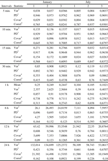
Table 1 - Historical values observed (1), estimated by the models (2) and obtained by the generated series (3) of rainfall in intervals of 5 minutes for the months of January and July.
1Mean –mean precipitation in 1-hour interval (mm); 2 Var – variance of precipitation in thinterval (mm²); 3 PD – probability of the interval being dry; 4Covar – autocovariance with lag 1 (mm²); 5Correl – autocorrelation coeficient with lag 1.
2) Each rain event has a number h associated with it that speciies the intensity of the rain. These numbers are independent random variables with a gamma distribution of mean a/u, and variance a/u2;
3) Each rain consists of one or more cells. The irst cell starts at the time of origin of rain and subsequent cells have time to start the According Poisson process with rate b (b = kh ) h-1,
after time exponentially distributed with mean 1/ϒ (ϒ= fh) h no
further cell begins;
4) Each cell is a rectangular pulse of rain with intensity exponentially distributed with mean mx mm h-1, and duration
exponentially distributed, with mean 1/h h.
5) The total precipitation is given by the sum of all the cells and all the rain.
A computer program in Delphi was written to generate a series of rain events as well as to calculate the statistics deined by Equations 2 to 6.
3. RESULTS AND DISCUSSION
The performance of the model can be evaluated by comparing the moments of the model to the characteristic historic values. In Table 1 can be found values of the statistics of the precipitation in intervals of 5, 10, 15, 30 min., 1 hour (60 min.),
1 2 3 1 2 3
5 min. Var2 0,038 0,037 0,0366 0,005 0,004 0,0037 PD3 0,946 0,973 0,9762 0,962 0,969 0,9691 Covar4 0,029 0,031 0,0302 0,004 0,004 0,0035 Correl5 0,765 0,825 0,8241 0,787 0,937 0,9301 10 min. Var2 0,135 0,136 0,1337 0,017 0,015 0,0144 PD3 0,929 0,967 0,9704 0,951 0,965 0,9663 Covar4
0,087 0,096 0,0938 0,012 0,013 0,0127 Correl5
0,645 0,703 0,7005 0,717 0,887 0,8797 15 min. Var2 0,271 0,281 0,2766 0,035 0,032 0,0314
PD3
0,917 0,96 0,9648 0,944 0,962 0,9638 Covar4 0,154 0,172 0,1689 0,024 0,027 0,0263 Correl5 0,568 0,613 0,6093 0,689 0,847 0,8372 30 min. Var2 0,85 0,908 0,8921 0,12 0,119 0,1155 PD3 0,892 0,783 0,9482 0,929 0,942 0,9573 Covar4 0,353 0,404 0,3888 0,076 0,09 0,0862 Correl5 0,415 0,445 0,4338 0,63 0,76 0,7449 1 h Mean 1 0,25 0,249 0,2447 0,104 0,105 0,1021 Var2 2,357 2,625 2,5684 0,39 0,418 0,4037 PD3 0,857 0,91 0,9178 0,908 0,941 0,9471 Covar4 0,738 0,778 0,7111 0,242 0,275 0,2583 Correl5
0,313 0,296 0,2743 0,62 0,658 0,6371 6 h Var2 26,1 26,493 24,8159 7,111 8,094 7,5957
PD3
0,696 0,695 0,7134 0,813 0,863 0,8755 Covar4
4,27 3,505 3,0243 3,655 3,181 2,7939 Correl5 0,164 0,132 0,123 0,514 0,393 0,3607 12 h Var2
63,42 59,996 55,5548 21,942 22,55 20,8764 PD3 0,608 0,546 0,5659 0,76 0,784 0,8011 Covar4 5,699 7,353 7,0806 7,926 6,822 5,7372 Correl5 0,09 0,123 0,1265 0,361 0,303 0,2632 24 h Var2 132,014 134,699 125,2372 58,109 58,743 53,0617 PD3 0,421 0,356 0,3744 0,661 0,646 0,6707 Covar4 21,392 14,498 11,5193 11,588 13,305 10,1949 Correl5 0,162 0,108 0,0921 0,199 0,226 0,18 Intervals Statístic
0 20 40 60 80 100 120 140
1 10 100 1000 10000
V a r ia n c e ( m m ²) Duration (min)
Ja nua ry
Observed Simula ted 0 50 100 150 200 250
1 10 100 1000 10000
V a r ia n c e ( m m ²) Duration (min) Februa ry Observed Simula ted 0 10 20 30 40 50 60 70 80 90 100
1 10 100 1000 10000
V a r ia n c e (m m ²) Duration (min) Ma rch Observed Simula ted 0 10 20 30 40 50 60 70
1 10 100 1000 10000
V a r ia n c e ( m m ²) Duration (min) April Observed Simula ted 0 20 40 60 80 100 120 140
1 10 100 1000 10000
V a r ia n c e (m m ²) Duration (min) Ma y Observed Simula ted 0 10 20 30 40 50 60 70
1 10 100 1000 10000
V a r ia n c e ( m m ²) Duration (min) June Observed Simula ted 0 10 20 30 40 50 60 70 80 90
1 10 100 1000 10000
V a r ia n c e ( m m ²) Duration (min) July Observed Simula ted 0 10 20 30 40 50 60 70 80 90
1 10 100 1000 10000
V a r ia n c e ( m m ²) Duration (min) August Observed Simula ted 0 10 20 30 40 50 60 70 80 90 100
1 10 100 1000 10000
V a r ia n c e ( m m ²) Duration (min) September Observed Simula ted 0 20 40 60 80 100 120
1 10 100 1000 10000
V a r ia n c e ( m m ²) Duration (min) October Observed Simula ted 0 10 20 30 40 50 60 70 80 90 100
1 10 100 1000 10000
V a r ia n c e ( m m ²) Duration (min) November Observed Simula ted 0 20 40 60 80 100 120 140 160 180
1 10 100 1000 10000
V a r ia n c e (m m ²) Duration (min) December Observed Simula ted
0,0 0,1 0,2 0,3 0,4 0,5 0,6 0,7 0,8 0,9 1,0
1 10 100 1000 10000
PD Duration (min) Janua ry Observed Simulated 0,0 0,1 0,2 0,3 0,4 0,5 0,6 0,7 0,8 0,9 1,0
1 10 100 1000 10000
PD Duration (min) February Observed Simula ted 0,0 0,1 0,2 0,3 0,4 0,5 0,6 0,7 0,8 0,9 1,0
1 10 100 1000 10000
PD Duration (min) March Observed Simulated 0,0 0,1 0,2 0,3 0,4 0,5 0,6 0,7 0,8 0,9 1,0
1 10 100 1000 10000
PD
Duration (min)
April Observed Simulated 0,0 0,1 0,2 0,3 0,4 0,5 0,6 0,7 0,8 0,9 1,0
1 10 100 1000 10000
PD Duration (min) May Observed Simula ted 0,0 0,1 0,2 0,3 0,4 0,5 0,6 0,7 0,8 0,9 1,0
1 10 100 1000 10000
PD Duration (min) June Observed Simulated 0,0 0,1 0,2 0,3 0,4 0,5 0,6 0,7 0,8 0,9 1,0
1 10 100 1000 10000
PD Duration (min) July Observed Simulated 0,0 0,1 0,2 0,3 0,4 0,5 0,6 0,7 0,8 0,9 1,0
1 10 100 1000 10000
PD Duration (min) August Observed Simula ted 0,0 0,1 0,2 0,3 0,4 0,5 0,6 0,7 0,8 0,9 1,0
1 10 100 1000 10000
PD Duration (min) September Observed Simulated 0,0 0,1 0,2 0,3 0,4 0,5 0,6 0,7 0,8 0,9 1,0
1 10 100 1000 10000
PD Duration (min) October Observed Simulated 0,0 0,1 0,2 0,3 0,4 0,5 0,6 0,7 0,8 0,9 1,0
1 10 100 1000 10000
PD Duration (min) November Observed Simula ted 0,0 0,1 0,2 0,3 0,4 0,5 0,6 0,7 0,8 0,9 1,0
1 10 100 1000 10000
PD
Duration (min)
December
Observed
Simulated
6 hours (360 min.), 12 hours (720 min.), and 24 hours (1440) minutes for the observed series(1) and simulated series (3), as well as the theoretical values of the model (2) for the months of January and July. It is observed that in a general way the modiied Bartlett-Lewis model applied for durations of less than 1 hour simulated the rainfall series, maintaining the values of the irst and second moments over diverse levels of accumulation.
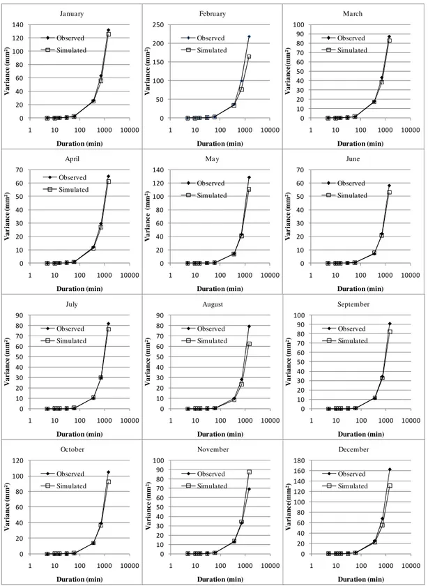
In Figure 2 are represented the values of variance for the precipitation in intervals of 5, 10, 15, 30 min., 1 hour (60 min.), 6 hours (360 min.), 12 hours (720 min.), and 24 hours (1440) minutes of the observed series and a simulated series of 100 years with intervals of 5 minutes. In the majority of months it can be veriied that the values of the simulated series and the observed series are very close, principally for the smallest intervals of duration. In the month of February it is observed that for durations of 12 and 24 hours the simulated series showed less variance than the observed series.
Also, in the months of August and December the variance of the rainfall in periods of 24 hours in the simulated series was less than in the observed series. It is important to note that the observed series has 27 years of observation - since some months were excluded in the analysis due to the presence of failures in the registers – and the simulated series contains 100 years of observation. This can explain in part the lesser variance in the simulated series.
In Figure 3 are shown the values of the probability of the interval being dry in .the observed precipitation series, and in a series of 100 simulated years with an interval of 5 minutes. It can be seen that in the simulated series, larger values of probability of the interval being dry are found. In the mean these differences are less than 5%, although in the months of May and September there appeared differences in the probabilities greater than 10% for intervals equal to or greater than 6 hours.
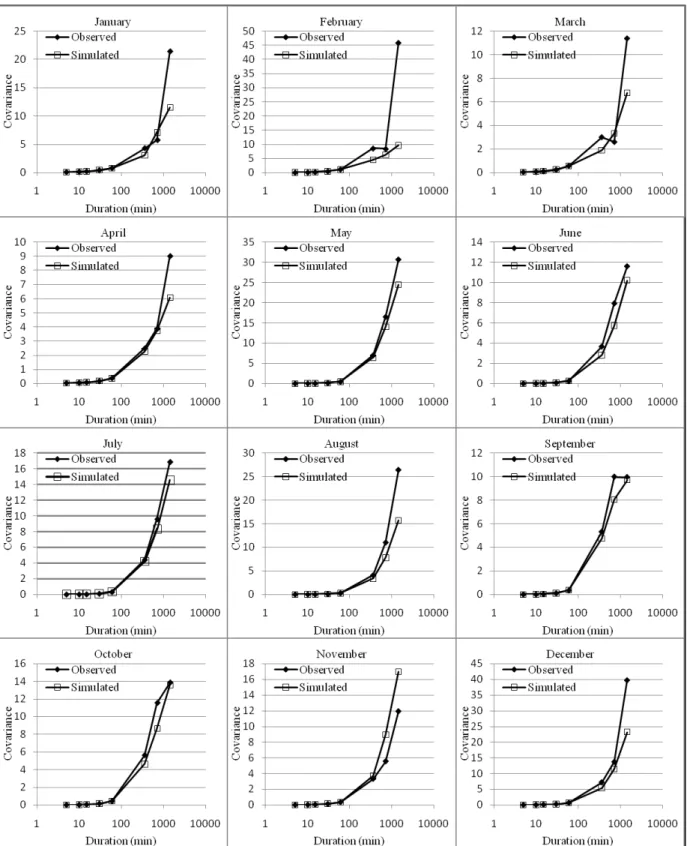
In Figure 4 are represented the values of covariance in the series of observed precipitation and a series of 100 simulated years with intervals of 5 minutes. It can be seen that for intervals of duration up to 12 hours there is similarity between the observed and simulated values. For the series aggregated over 24 hours of duration it can be seen that the simulated series tend to show smaller values of autocovariance, with the largest differences being observed during the months of February, March, April and December. The large discrepancy observed during the month of February can be attributed in part to the presence of extreme values in the observed series that are relected in the high values of variance and autocovariance.
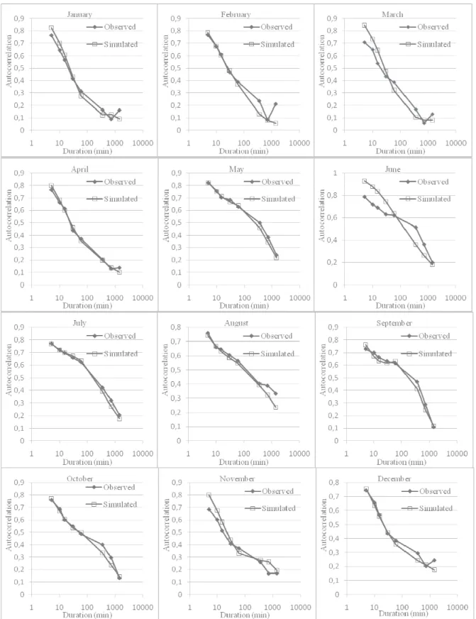
In Figure 5 are represented the values of autocorrelation of the precipitation in the observed series and a series of 100 simulated years with interval 5 minutes. It can be seen that in a general manner the values of the simulated series maintain the characteristics of the observed series for all of the intervals
of aggregation. One observes that the simulated series exhibits an inverse relation between the values of autocorrelation and duration, and in the observed series it is seen that in the months of December to March the values of autocorrelation for the 24-hour interval are greater than the values for the 12-hour interval. This behavior could be due to the atypical values of covariance in the observed series.
In Figure 6 are found the values of monthly mean intensity for the observed and simulated series. The capacity of the model to preserve the irst-order moments is evident. The differences observed between the monthly means of the observed and simulated series were less than 5%, demonstrating the adequacy of the model in simulating showers of short duration. The seasonal variation of all the statistics of the observed and simulated series show the necessity of considering the seasonal variation of the parameters for each month.
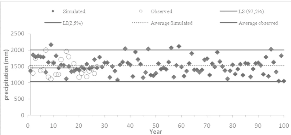
Figures 7 and 8 show the rainfall totals in intervals of 1 hour and 5 minutes for the observed series and the simulated series of 100 years duration, together with the conidence interval of 95%. It can be seen also in the annual totals that the model simulates the rainfall, maintaining the characteristics of the observed series, with similar form for the hourly as well as for the 5-minute intervals. Among the few papers applying the rectangular pulse model for durations less than 1 hour, the work of Damé stands out: Here the parameters of the model were adjusted with data from Pelotas (Rio Grande do Sul) and the method applied to the simulation of a rainfall series with intervals of 15 minutes. Since the it of the model parameters relecting the seasonal differences maintains the structural characteristics consistent with the occurrence of the principal types of rain, and still considering that the simulated series present statistics similar to the observed series, it can be concluded that this mathematical model of rain is an important tool that can be employed in hydrologic studies that require long series of precipitation data in intervals of duration of less than 1 day. Taking as a base the values of the mean, variance and autocorrelation, it can be said that the results obtained agree with the work of Rodriguez-Iturbe (1997), Verhoest et al. (1997) who observed that the model preserves the irst moments. The possibility of using the series of data observed over relatively short periods to adjust the parameters of the model and subsequently generate long series of rainfall data represents an advance in hydrologic studies.
4. CONCLUSIONS
Figure 6 - Mean monthly intensity for the observed and simulated series.
Figure 7 - Annual totals of rainfall for the 1-hour series with upper and lower limits for a 95% conidence interval.
2) There was observed a general tendency to overestimate the probabilities of periods being dry and to underestimate the covariance for intervals of 24 hours, principally in the summer;
3) The annual rainfall totals simulated for all the intervals of duration analyzed remained within a conidence interval of 95%;.
4) The modiied Bartlett-Lewis model makes possible the simulation of rainfalls with intervals of duration down to 5 minutes, preserving the statistical properties of the precipitation over various levels of temporal aggregation.
5. REFERENCES
ANDRADE JUNIOR, A. S.; FRIZZONE, J. A.; SENTELHAS, P. C. Simulação de precipitação diária para Parnaíba e Teresina, PI, em planilha eletrônica. Revista Brasileira de Engenharia Agrícola e Ambiental, v.5, n.2, p.271-278, 2001.
BACK, Á. J. Relações entre precipitação intensas de diferentes duração ocorridas no município de Urussanga, SC. Revista Brasileira de Engenharia Agrícola e Ambiental, v.13, n.2, p.170-175, 2009.
BACK, Á. J.; DORFMAN, R.; CLARKE, R. Modelagem da precipitação horária por meio do modelo de pulsos retangulares de Bartlett-Lewis modiicado. Revista Brasileira de Recursos Hídricos. , v.4, p.5 - 17, 1999.
CECILIO, R. A.; PRUSKI, F. F. Interpolação dos parâmetros de equações de chuvas intensas com uso do inverso de potências da distância. Revista Brasileira de Engenharia Agrícola e Ambiental, v.7, n.3, p.501-504, 2003.
COWPERTWAIT, P. S. P.; O’CONNELL, P. E.; METCALFE, A. V.; MAWDSLEY, J. A. Stochastic point process modeling of rainfall. I. Single-site and validation. Journal of Hydrology, v.175, 1996.
DAMÉ, R. C. F.; TEIXEIRA, C. F. A.; LORENSI, R. P. Simulação de precipitação com duração horária mediante o uso do modelo Bartlett-Lewis de pulos retangular modiicado. Revista Brasileira de Agrociência, v.13, n.1, p.13-18, 2007. DAMÉ, R. C. F.; PEDROTTI, C. B. M.; CARDOSO, M.
A.; SILVEIRA, C. P.; DUARTE, L. A.; MOREIRA, C. Comparação entre curvas Intensidade-Duração-Frequência de ocorrência de precipitação obtidas a partir de dados pluviográficos com aquelas estimadas por técnicas de desagregação de chuva diária. Revista Brasileira de Agrociência, v.12, n.4, p.505-509, 2006.
DAMÉ, R. C. F. Desagregação de precipitação diária para
estimativa de curvas intensidade-duração-freqüência.
2001.131f. Tese (Doutorado em engenharia de Recursos Hídricos e Saneamento Ambiental) – Instituto de Pesquisas Hidráulicas, Universidade Federal do Rio Grande do Sul, Porto Alegre, 2001.
DOURADO NETO, D.; ASSIS, J. P.; MAFRON, P. A.; SPAROVEK, G.; BARRETO, A. G. O. P.; MARTIN, T. N. Simulação estocástica de valores médios diários de temperatura do ar e de radiação solar global para Piracicaba-SP, utilizando a distribuição normal. Revista Brasileira de Agrometeorologia, v.13, n.2, p225-235, 2005.
ENTEKHABI, D.; RODRUGUEZ-ITUBE, I.; EAGLESON, P. S. Probabilistic representation of the temporal rainfall process by modiied Neyman-Scott rectangular pulses model: parameter estimation and validation. Water resources Research, Washington, v.25, 1989.
GENNEVILE, M. S.; BOOCK, A. Modelos estocásticos para simulação da precipitação pluviométrica diária de uma região. Pesquisa Agropecuária Brasileira, v.18, n.9, p.959-966. 1983.
KHALIQ, M. N.; CUNNANE, C. Modeling point rainfall occurrences with the Modiied Bartlett-Lewis Rectangular Pulses Model. Journal of Hydrology, v.180, 1996.
LAPPONI, J. C. Estatística usando Excel. 4 ed., rev. e atual. São Paulo: Elsevier, 2005.
LIMA, H. M. F.; MATA, I. P. LIMA, A. V. F. Aplicação e validação de um simulador estocástico de variáveis climáticas: o caso da precipitação. Ingenieria Del Água, v.12, n.1, p.27-37, 2005. MELLO, C. R.; SILVA, A. M. Modelagem estatística da
precipitação mensal e anual e no período seco para o estado de Minas Gerais. Engenharia Agrícola e Ambiental, v.13, n.1, p.68-74, 2009.
OLIVEIRA, V. P. S.; ZANETTI, S. S.; PRUSKI, F. F. CLIMABR Parte I: Modelo para a geração de séries sintéticas de precipitação. Revista Brasileira de Engenharia Agrícola e Ambiental, v.9, n.3, p.348-355, 2005.
OLIVEIRA, L. F. C.; ANTONINI, J. C.DOS A.; FIOREZE, A. P.; SILVA, M. A. S. Métodos de estimativa de precipitação máxima para o Estado de Goiás. Engenharia Agrícola e Ambiental. v.12, n.6, p.620-625, 2008
PEDROLLO, O. C. GEDAC: Gerenciamento de Dados
Contínuos. Manual do usuário. IPH vol. 34. Porto Alegre,
1997, 60 p.
RODRIGUEZ-ITURBE, I. Scale of luctuation of rainfall models.
Water Resources Research. v. 22, n.9, 1988.
RODRIGUEZ-ITURBE, I. Some models for rainfall based on stochastic point process. Proc. R. Soc. Lond,. v.410, 1987.