Integrating Recent Land Cover Mapping Efforts to Update the National Gap Analysis
Program’s Species Habitat Map
Alexa J. McKerrowa, Anne Davidsonb, Todd S. Earnhardt c and Abigail L. Bensond
a
U.S. Geological Survey, Core Science Analytics, Synthesis & Libraries, Raleigh, NC 27695-7617 [email protected] b
University of Idaho, College of Natural Resources Moscow, ID 83843 [email protected] c
North Carolina State University, Department of Applied Ecology, Raleigh, NC 27695-7617 [email protected] d
U.S. Geological Survey, Core Science Analytics, Synthesis & Libraries, Denver, CO 80225-0046 [email protected]
KEY WORDS: GAP; LANDFIRE; NLCD; Land Cover; Habitat
ABSTRACT:
Over the past decade, great progress has been made to develop national extent land cover mapping products to address natural resource issues. One of the core products of the GAP Program is range-wide species distribution models for nearly 2000 terrestrial vertebrate species in the U.S. We rely on deductive modeling of habitat affinities using these products to create models of habitat availability. That approach requires that we have a thematically rich and ecologically meaningful map legend to support the modeling effort. In this work, we tested the integration of the Multi-Resolution Landscape Characterization Consortium’s National Land Cover Database 2011 and LANDFIRE’s Disturbance Products to update the 2001 National GAP Vegetation Dataset to reflect 2011 conditions. The revised product can then be used to update the species models.
We tested the update approach in three geographic areas (Northeast, Southeast, and Interior Northwest). We used the NLCD product to identify areas where the cover type mapped in 2011 was different from what was in the 2001 land cover map. We used Google Earth and ArcGIS base maps as reference imagery in order to label areas identified as “changed” to the appropriate class from our map legend. Areas mapped as urban or water in the 2011 NLCD map that were mapped differently in the 2001 GAP map were accepted without further validation and recoded to the corresponding GAP class. We used LANDFIRE’s Disturbance products to identify changes that are the result of recent disturbance and to inform the reassignment of areas to their updated thematic label. We ran species habitat models for three species including Lewis’s Woodpecker (Melanerpes lewis) and the White-tailed Jack Rabbit (Lepus townsendii) and Brown Headed nuthatch (Sitta pusilla). For each of three vertebrate species we found important differences in the amount and location of suitable habitat between the 2001 and 2011 habitat maps. Specifically, Brown headed nuthatch habitat in 2011 was -14% of the 2001 modeled habitat, whereas Lewis’s Woodpecker increased by 4%. The white-tailed jack rabbit (Lepus townsendii) had a net change of -1% (11% decline, 10% gain). For that species we found the updates related to opening of forest due to burning and regenerating shrubs following harvest to be the locally important main transitions. In the Southeast updates related to timber management and urbanization are locally important.
INTRODUCTION
The National Gap Analysis Program seeks to provide the land management and conservation agencies of the United States with information that allows them to effectively manage and conserve the nation's biological resources (Aycrigg et al. 2013; Boykin et al. 2013). Towards this end GAP produces three main digital data products; an inventory of protected lands, a map of ecological systems and habitat distribution models for the country’s terrestrial vertebrate species. In support of that effort, an ecologically meaningful land cover map with high thematic resolution was developed based on 2001 era Landsat satellite imagery.
The National GAP Land Cover dataset reflects the work of several different projects brought together to create a seamless dataset for the conterminous U.S. Data from four regional GAP projects (Southwest, Southeast, Northwest, and California) were brought together with LANDFIRE Program Existing Vegetation Data for the
Northeast and Midwest regions to create the 2001 land cover product. The map legend is based on the Ecological Systems Classification (Comer et al. 2003), with modifiers added to accommodate variations in the systems that would be important for refining species habitat models. For example, we included two variants of the Southern Piedmont Dry Oak-(Pine) Forest, realizing that the pine dominated expression of that system would support a different suite of species and would represent a significant area in the Southeast region. There were a total of 578 map classes in the conterminous U.S., of those 551 describe natural systems and 27 represent anthropogenic map classes (e.g. row crop, developed) or areas that have been recently disturbed (e.g. harvested, recently burned, introduced).
2011 conditions. While land cover change represents a relatively small proportion of the landscape, it can be highly significant locally with important implications for species distribution modelling. We explored the feasibility of updating the 2001 land cover dataset using the 2011 NLCD and LANDFIRE Disturbance datasets and used that information to determine the potential impact of this update on habitat suitability modeling for three wide-ranging habitat specialists.
METHODS
The coterminous United States has been divided into 9 geographic areas (geoareas; Figure 1). These geoareas are aggregations of the 66 Multi-Resolution Land Characteristics Consortium (MLRC mapping zones that have been used by NLCD, GAP and LANDFIRE as mapping zones in their 2001 national mapping efforts (Homer et al. 2004). We selected three of the nine geoareas in the United States as pilot areas for this project, Inland Northwest, Southeast, and Northeast. The remaining six geoareas will be updated using similar methods in the next few months with a goal of publishing an updated National GAP Land Cover Dataset in early 2015.
For each geoarea we used the ArcGIS Combine operation to generate pixel combinations of 2001
National GAP Vegetation data (USGS GAP 2011), 2011 NLCD (Jin et al. 2013), 2010 LANDFIRE disturbance data (Nelson et al. 2013), and ultimately the 10-digit Hydrologic Unit Code (HUC) data from the USGS Watershed Boundary Dataset (USGS WBD 2011). This operation generated raster attribute tables with hundreds of thousands of records for each geoarea (Southeast 698,688; Northeast 487,690; and Inland Northwest 194,208). The 2011 NLCD label was accepted into the GAP update layer for row crop, pasture/hay, water, and the four developed land cover classes without further investigation. We kept the 2001 GAP data class label if it matched the NLCD general land cover class. For example, for pixels mapped as Atlantic Coastal Plain Dry and Dry-Mesic Oak Forest in the 2001 GAP map that were mapped as deciduous forest in the NLCD 2011 map; we maintained the original 2001 ecological system call. For combinations where the NLCD 2011 cover class was not consistent we used the vegetation and disturbance information and high resolution imagery from Google Earth or ArcGIS base maps to assign the updated 2011 cover class. For example, in the Inland Northwest combinations that were a forest type in the 2001 GAP map, shrub in the NLCD 2011 map and had been burned according to the 2010 LANDFIRE disturbance data were assigned to the class Recently Burned Forest in the 2011 GAP update.
After accepting the 2011 NLCD labels for agriculture, water, and developed classes as well as the ecological system matches, there were a large number of combination records remaining. The combination dataset allowed each analyst to visualize the distribution of the pixels within the un-assigned combinations and evaluate the potential source of difference between the two dates. Prior to adding the 10-digit HUC information, we observed that certain GAP-NLCD-disturbance combinations represented different transitions depending on where it occurred in the geoarea. Thus the 10-digit HUC was added to provide more flexibility in assigning labels to the transitions/updates in different parts of the geoarea. This came at a cost of more records overall but many of the resulting combinations were represented by only a few pixels and were ignored in the analysis. We did not use a hard pixel count threshold for determining which combinations were considered for generating a recode rule. Instead we used information about the distribution and pattern of the combination, as well as the type of transition to prioritize which combinations were evaluated for recoding at this step.
Following the initial recode, there were still combinations that remained unassigned. These cases were typically combinations represented by single and small groups of pixels scattered across one or more HUC’s or a combination whose recode options included several possible ecological systems. In these situations, we used the land cover classes in proximity to the unassigned pixels to drive the labeling process. An example would be a pixel mapped as non-forest in the 2001 GAP map that was to be recoded to a forest class in the updated map but there were multiple options for the final forest class label. In this case, we would apply a neighborhood majority or expand function for that pixel to determine forest type and assign that type to the pixel. The neighborhood operations were constrained to certain forest types. For example, if the NLCD 2011 class was Woody Wetland, only wetland Ecological Systems were used in determining the potential classes for the recode. Another example from the Inland Northwest is the shrub ecological system in the 2001 GAP map, that was mapped as forest in the 2011 NLCD and had no disturbance noted in the LANDFIRE disturbance data. A review of the imagery at several locations confirmed that the areas were indeed forested, so those pixels were labeled using the geographically appropriate forest type based on the nearby forested systems.
For pixels that remained unassigned after proximity assignments, we defaulted to the 2001 GAP map assignments. This occurred for areas where the accounted for a very small number of pixels or when the physiognomy type indicated by the combination was very geographically isolated, for example an island of forest in a grassland, such that it was not feasible to cover it through the use of the neighborhood or majority functions.
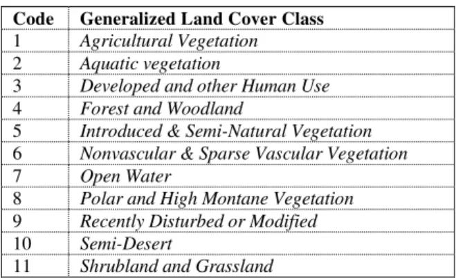
Once the update was complete a crosswalk from the full 578 map legend to 11 general land cover classes was created In order to summarize general trends in the data (Table 1).
Table 1. List of the 11 General Land Cover Classes used for summarizing the results.
Code Generalized Land Cover Class 1 Agricultural Vegetation 2 Aquatic vegetation
3 Developed and other Human Use 4 Forest and Woodland
5 Introduced & Semi-Natural Vegetation 6 Nonvascular & Sparse Vascular Vegetation 7 Open Water
8 Polar and High Montane Vegetation 9 Recently Disturbed or Modified 10 Semi-Desert
11 Shrubland and Grassland
Species Modeling
To explore the impact of the update on the species modeling effort, we used ArcGIS to run the National Gap Species Habitat Models with both the 2001 and the 2011 land cover maps (USGS GAP 2013). We ran models for three species including Lewis’s Woodpecker (Melanerpes lewis) and the White-tailed Jack Rabbit (Lepus townsendii) in the Interior Northeast and Brown headed nuthatch (Sitta pusilla) in the Southeast. The three species represent wide-ranging habitat specialists. For example, the Brown headed nuthatch occurs in pine forests and woodlands throughout the Southeast. Spatial summaries of habitat loss and gain were calculated using Python scripting. Three calculations were done for each species, the number of pixels of suitable habitat in 2001 that remained suitable in 2011, the number of pixels that were added in 2011, and the number of pixels that became unsuitable between the two dates. The percent change was based on the 2001 habitat model; Equation 1 provides an example for calculating the net change.
Net change = (2001 km2 -2011 km2)/2001 km2 * 100) (1)
To determine which land cover transitions impacted the species models the most, the script calculated the land cover transitions that contributed to the gains and losses. We used the results to discuss the most extensive land cover updates that contributed to the losses and gains for each species.
RESULTS Land Cover
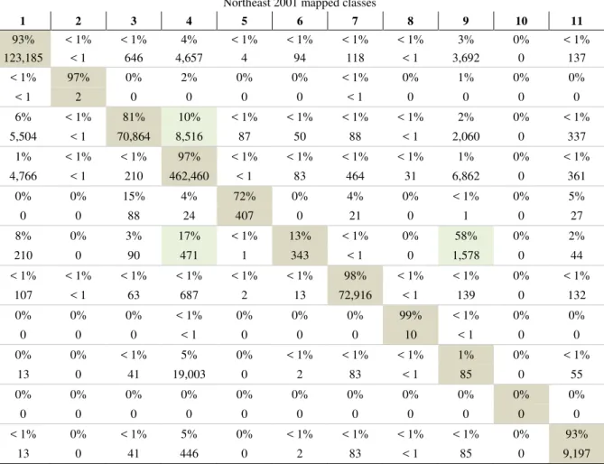
In the Northeastern geoarea, 7.74% (63,122 km2) of the area was mapped to a different general land cover class between the 2001 and 2011 maps (Table 2b). The largest shift in areas between mapped categories were represented by a shift of Forest and Woodland pixels in 2001 to Recently Disturbed/modified (19,003 km2
), Developed & Other Human Uses (8,515 km2), and Agricultural Vegetation (4,657 km2) in the 2011 map. The second most common difference occurred within the Agricultural Vegetation with 5,504 km2 being mapped as Developed and Other Human Use and 4,766 km2 in the Forest and Woodland categories in the 2011 map.
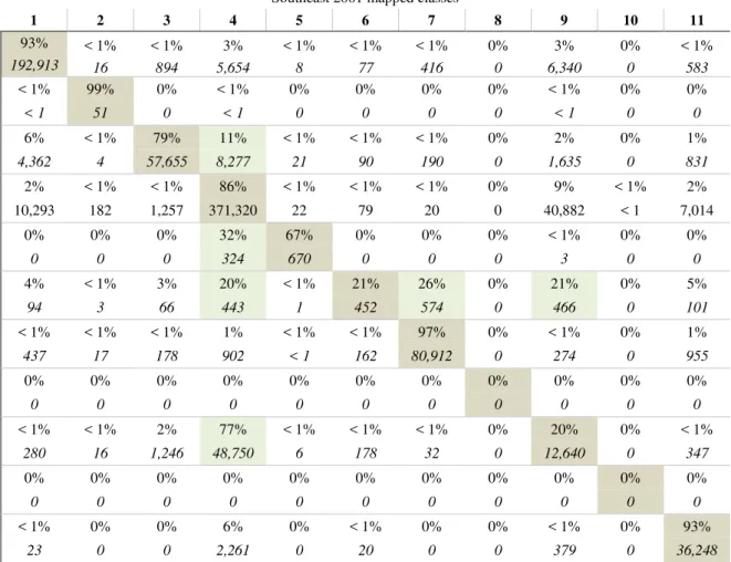
In the Southeast geoarea, 16.4% (147,686 km2) was mapped to a different general land cover class between the 2001 and 2011 maps (Table 2c) and 48,750 km2 of the Forest and Woodland class in 2001 was mapped as Recently Disturbed/Modified in the 2011 land cover map. Changes in the urban classes represent another substantial shift with Agricultural Vegetation (4,362 km2) and Forest and Woodland (8,277 km2) in 2001 being mapped in the Developed and Other Human Use Class in 2011.
Table 2a. Percent and area (km2) for each general land cover class in the 2001 and 2011 maps for the Inland Northweset geoarea. Codes correspond to the land cover classes in Table 1. Diagonals are highlighted for ease of reading, and off diagonals are highlighted where greater than 10% of the 2001 General Land Cover Class was different in 2011
In
lan
d
No
rt
h
we
st 2
0
1
1
m
ap
p
ed
c
la
ss
es
Inland Northwest 2001 mapped classes
1 2 3 4 5 6 7 8 9 10 11
1 86% 0% 2% 3% < 1% < 1% < 1% < 1% < 1% 2% 7%
9,072 0 227 282 6 < 1 9 < 1 7 174 764
2 0% 0% 0% 0% 0% 0% 0% 0% 0% 0% 0%
0 0 0 0 0 0 0 0 0 0 0
3 8% 0% 68% 7% < 1% < 1% < 1% < 1% < 1% 6% 11%
292 0 2,529 259 7 1 14 < 1 7 210 393
4 < 1% 0% < 1% 90% < 1% < 1% < 1% < 1% 4% 1% 4%
194 0 172 155,858 33 183 142 574 6,116 2,480 6,641
5 0% 0% 0% 0% 41% 0% 0% 0% 3% 56% 0%
0 0 0 0 417 0 0 0 34 566 0
6 0% 0% < 1% 3% 0% 89% < 1% < 1% < 1% 5% 3%
0 0 < 1 69 0 2,049 1 3 < 1 109 63
7 < 1% 0% < 1% 4% < 1% < 1% 91% < 1% < 1% 1% 3%
10 0 12 175 < 1 3 3,895 11 2 53 112
8 0% 0% < 1% 1% 0% 4% 0% 93% < 1% < 1% 1%
0 0 < 1 132 0 353 0 8,258 < 1 20 94
9 0% 0% 0% 41% 0% 0% 0% < 1% 53% 4% 1%
0 0 0 6,805 0 0 0 6 8,796 744 237
10 0% 0% < 1% 0% 0% 0% 0% < 1% < 1% 95% 5%
0 0 118 0 0 0 0 147 10 47,743 2,433
11 < 1% 0% < 1% 23% < 1% < 1% < 1% < 1% < 1% 4% 72%
68 0 376 13,139 12 < 1 21 276 56 2,154 41,186
Species Models
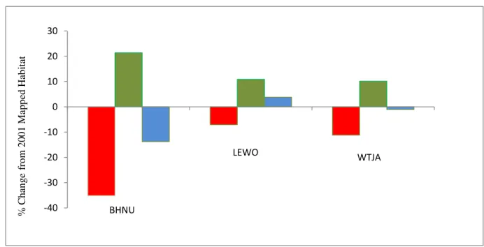
Each of the species models showed that the changes in the land cover map did impact the amount of modeled habitat. Specifically, Brownheaded Nuthatch, and White-tailed Jack-Rabbit showed a net loss in predicted habitat, while Lewis’s Woodpecker showed a net gain (Figure 2).
mapped as East Gulf Coastal Plain Interior Upland Longleaf Pine Woodland - Loblolly Modifier in 2001 were remapped as Southern Coastal Plain Blackwater River Floodplain Forest. The habitat gains were from the reverse of the previously described vectors with evergreen forest regenerating on harvested timber areas. Increase in the developed classes represented approximately ~4% (3,407 km2) of the decreased in total habitat mapped.
Lewis’s woodpecker is typically found in open forests and it has a tendency to nest in burned landscapes (Abele et al. 2004). Overall modeled habitat for the Lewis’s Woodpecker increased in area by 3.81% (5,933 km2) between 2001 and 2011 in the Inland Northwest maps. Two updates that resulted in the largest area of habitat increase were the, Harvested Forest - Northwestern Conifer Regeneration to Northern Rocky Mountain Dry-Mesic Montane Mixed Conifer Forest, and the reclassification of Rocky Mountain Aspen Forest and Woodland to Middle Rocky Mountain Montane Douglas-fir Forest and Woodland. The two changes that resulted in the greatest decreases in modeled habitat were Northern Rocky Mountain Dry-Mesic Montane Mixed
Conifer Forest to Northern Rocky Mountain Montane-Foothill Deciduous Shrubland and Northern Rocky Mountain Mesic Montane Mixed Conifer Forest to Northern Rocky Mountain Montane-Foothill Deciduous Shrubland. Based on the reference imagery these mapped changes include forest disturbance such as harvest and wildfire that were not captured by the LANDFIRE disturbance layer and a difference in the breaks between forest and shrub physiognomies employed by GAP in the 2001 map and NLCD in their 2011 map.
Habitat for the White-tailed Jack Rabbit includes prairie and montane herbaceous areas among scattered evergreens (Flux and Angermann 1990). The White-tailed Jack Rabbit model had a net loss of 1.08% of the modeled habitat between the two maps. The largest increases were the result of transitions from Rocky Mountain Subalpine Dry-Mesic Spruce-Fir Forest and Woodland and Rocky Mountain Lodgepole Pine Forest to the Recently burned forest class. The largest loss of modeled habitat came from the mapped change in structure of Harvested Forest - Grass/Forb Regeneration to Harvested Forest - Shrub Regeneration.
Table 2b. Percent and area (km2) for each general land cover class in the 2001 and 2011 maps for the Northeast geoarea. Codes correspond to the land cover classes in Table 1. Diagonals are highlighted for ease of reading, and off diagonals are highlighted where greater than 10% of the 2001 General Land Cover Class was different in 2011.
Northeast 2001 mapped classes
1 2 3 4 5 6 7 8 9 10 11
93% < 1% < 1% 4% < 1% < 1% < 1% < 1% 3% 0% < 1%
123,185 < 1 646 4,657 4 94 118 < 1 3,692 0 137
< 1% 97% 0% 2% 0% 0% < 1% 0% 1% 0% 0%
< 1 2 0 0 0 0 < 1 0 0 0 0
6% < 1% 81% 10% < 1% < 1% < 1% < 1% 2% 0% < 1%
5,504 < 1 70,864 8,516 87 50 88 < 1 2,060 0 337
1% < 1% < 1% 97% < 1% < 1% < 1% < 1% 1% 0% < 1%
4,766 < 1 210 462,460 < 1 83 464 31 6,862 0 361
0% 0% 15% 4% 72% 0% 4% 0% < 1% 0% 5%
0 0 88 24 407 0 21 0 1 0 27
8% 0% 3% 17% < 1% 13% < 1% 0% 58% 0% 2%
210 0 90 471 1 343 < 1 0 1,578 0 44
< 1% < 1% < 1% < 1% < 1% < 1% 98% < 1% < 1% 0% < 1%
107 < 1 63 687 2 13 72,916 < 1 139 0 132
0% 0% 0% < 1% 0% 0% 0% 99% < 1% 0% 0%
0 0 0 < 1 0 0 0 10 < 1 0 0
0% 0% < 1% 5% 0% < 1% < 1% < 1% 1% 0% < 1%
13 0 41 19,003 0 2 83 < 1 85 0 55
0% 0% 0% 0% 0% 0% 0% 0% 0% 0% 0%
0 0 0 0 0 0 0 0 0 0 0
< 1% 0% < 1% 5% 0% < 1% < 1% < 1% < 1% 0% 93%
Table 2c. Percent and area (km2) for each general land cover class in the 2001 and 2011 maps for the Northeast geoarea. Codes correspond to the land cover classes in Table 1. Diagonals are highlighted for ease of reading, and off diagonals are highlighted where greater than 10% of the 2001 General Land Cover Class was different in 2011.
Southeast 2001 mapped classes
1 2 3 4 5 6 7 8 9 10 11
93% < 1% < 1% 3% < 1% < 1% < 1% 0% 3% 0% < 1%
192,913 16 894 5,654 8 77 416 0 6,340 0 583
< 1% 99% 0% < 1% 0% 0% 0% 0% < 1% 0% 0%
< 1 51 0 < 1 0 0 0 0 < 1 0 0
6% < 1% 79% 11% < 1% < 1% < 1% 0% 2% 0% 1%
4,362 4 57,655 8,277 21 90 190 0 1,635 0 831
2% < 1% < 1% 86% < 1% < 1% < 1% 0% 9% < 1% 2%
10,293 182 1,257 371,320 22 79 20 0 40,882 < 1 7,014
0% 0% 0% 32% 67% 0% 0% 0% < 1% 0% 0%
0 0 0 324 670 0 0 0 3 0 0
4% < 1% 3% 20% < 1% 21% 26% 0% 21% 0% 5%
94 3 66 443 1 452 574 0 466 0 101
< 1% < 1% < 1% 1% < 1% < 1% 97% 0% < 1% 0% 1%
437 17 178 902 < 1 162 80,912 0 274 0 955
0% 0% 0% 0% 0% 0% 0% 0% 0% 0% 0%
0 0 0 0 0 0 0 0 0 0 0
< 1% < 1% 2% 77% < 1% < 1% < 1% 0% 20% 0% < 1%
280 16 1,246 48,750 6 178 32 0 12,640 0 347
0% 0% 0% 0% 0% 0% 0% 0% 0% 0% 0%
0 0 0 0 0 0 0 0 0 0 0
< 1% 0% 0% 6% 0% < 1% 0% 0% < 1% 0% 93%
23 0 0 2,261 0 20 0 0 379 0 36,248
DISCUSSION
For this effort we are taking advantage of three national datasets to conduct a one-time update of our land cover map. In the process we leverage a thematically detailed Ecological Systems Map (National Gap Land Cover), the current land cover (NLCD), and the pattern of disturbance (LANDFIRE Disturbance) to create a 2011 era ecologically meaningful land cover map. This update will represent a significant resource for updating the GAP species models, while working towards the next generation land cover maps in collaboration with the LANDFIRE and NLCD Programs.
It is important to keep in mind that this work represents an update and not necessarily an exact change detection of the National Gap Land Cover map. Differences between the 2001 and 2011 map do not always represent on-the-ground changes in vegetation communities. Some of the differences are the result from the update of a class that was mis-classified in the original 2001 map. An area that contained the same vegetation in 2001 and 2011 but was incorrectly mapped in 2001 would show up as “changed” using our method. Varying techniques used across the mapping programs define vegetative communities may also contribute to differences. For
definition) mapped as shrub in the NLCD layer are best mapped as the Northern Rocky Mountain Ponderosa Pine Woodland and Savanna ecological system in the GAP map. While care was taken to avoid erroneous changes, some of the 13.9 % of the 2001 distribution of Northern Rocky Mountain Ponderosa Pine Woodland and Savanna in the Inland Northwest that was changed to Northern Rocky Mountain Montane Foothill and Deciduous Shrubland may be a result of this difference in the ecotone breaks.
disturbance, within a subset of the HUCs. While the initial steps result in a database in which each recode for a combination is captured, with the number of records in each geoarea it would be difficult to effectively summarize the logic behind every recode decision. While some issues with pattern and the concepts of ecological systems were dealt with through this process, the fact that we were working with combinations meant we were making decisions based on pixels and not pattern.
The results show that land use dynamics over a 10 year time-span do impact the models of predicted habitat suitability and reinforce the need for updating the land cover and the species models to better serve natural resource planning. Specifically, we found that forest harvest and regeneration, urbanization, and burning changed the amount and location of habitat for the three species we chose to highlight. For these wide ranging species with distinct habitat affinities the update in the land cover did have an impact on the modeled distribution. For habitat generalists we would expect the
impact of the update to be less, but still potentially locally relevant. Over time the ability to update the land cover through disturbance mapping and change detection should increase the efficiency of updates and subsequently the responsiveness to the natural resource community.
ACKNOWLEDGEMENTS
We would like to acknowledge the Core Science Synthesis, Analytics, Synthesis & Libraries’ National GAP Analysis Program for funding and Matt Rubino and Nathan Tarr of the North Carolina Cooperative Fish and Wildlife Research Unit, Department of Applied Spatial Ecology for help in implementing the species modeling. We thank Daniel Wieferich and Kurtis Nelson of USGS for helpful comments on early drafts of this document. Any use of trade, product, or firm names is for descriptive purposes only and does not imply endorsement by the U.S. Government.
Figure 2. Percent habitat lost (red), gained (green) and net change (blue) for Brown-headed Nuthatch (BHNU), Lewis's Woodpecker LEWO and White-tailed Jackrabbit (WTJA). Percentage based on 2001 habitat area.
-40 -30 -20 -10 0 10 20 30
% C
h
an
g
e
fr
o
m
2
0
0
1
Ma
p
p
ed
Hab
itat
BHNU
REFERENCES
Abele, S.C., V.A. Saab, and E.O. Garton. 2004.. Lewis’s Woodpecker (Melanerpes lewis): a technical
conservation assessment. [Online]. USDA Forest Service, Rocky Mountain Region.
[Online:http://www.fs.fed.us/r2/projects/scp/assessments /lewisswoodpecker.pdf]
Aycrigg, J. L., A. Davidson, L. Svancara, K. J. Gergely, A. McKerrow, and J. M. Scott. 2013. Representation of ecological systems within the protected areas network of the continental United States. PLoS ONE 8(1): e54689. Doi:10.1371/journal.pone.0054689.
Boykin, K., W. Kepner, D. Bradford, R. Guy, D. Kopp, A. Leimer, E. Samson, F. East, A. Neale, and K. Gergely. A National Approach for Mapping and Quantifying Habitat-based Biodiversity Metrics Across Multiple Spatial Scales . K. Boykin (ed.),
ECOLOGICAL INDICATORS. Elsevier Science Ltd, New York, NY, 33(0):139-147, (2013).
Comer, P., D. Faber-Langendoen, R. Evans, S. Gawler, C. Josse, G. Kittel, S. Menard, M. Pyne, M. Reid, K. Schulz, K. Snow, and J. Teague. 2003. Ecological Systems of the United States: A Working Classification of U.S. Terrestrial Systems. NatureServe, Arlington, Virginia.
Flux, J. E. C. and Angermann, R. 1990. Chapter 4: The Hares and Jackrabbits. In: J. A. Chapman and J. E. C. Flux (eds), Rabbits, Hares and Pikas: Status Survey and Conservation Action Plan, pp. 61-94. The World Conservation Union, Gland, Switzerland.
Homer, C., Huang, C., Yang, L., Wylie, B., Coan, M.,2004, Development of a 2001 National Land-Cover Database for the United States, Photogrammetric Engineering and Remote Sensing, 70, 7, 829-840.
Iglecia, M. N., J. A. Collazo, and A. J. McKerrow. 2012. Use of occupancy models to evaluate expert knowledge-based species-habitat relationships. Avian Conservation and Ecology 7(2): 5. http://dx.doi.org/10.5751/ACE-00551-070205
Jin, S., Yang, L., Danielson, P., Homer, C., Fry, J., and Xian, G. 2013. A comprehensive change detection method for updating the National Land Cover Database to circa 2011. Remote Sensing of Environment, 132: 159 –175.
Nelson , K. J., J. Connot, B. Peterson, J. J. Picotte. 2013. LANDFIRE 1020 – Updated Data to Support Wildfire and Ecological Management. Earthzine Sept 15, 2013. [Online: http://www.earthzine.org/2013/09/15/landfire- 2010-updated-data-to-support-wildfire-and-ecological-management/]
US Geological Survey, Gap Analysis Program (GAP). August 2011. National Land Cover, Version 2.[Online: http://gapanalysis.usgs.gov/gaplandcover/viewer/] U.S. Geological Survey Gap Analysis Program. 2013. Gap Analysis Program Species Distribution Models. [Online: