Professor, Institute of New Imaging Technologies, Universitat Jaume I, Castellón, Spain Dissertation co-supervised by

(1)

Nourhan Khalifa Abdelkareem

(2)

Analysis and Visualization of Energy use for University

Campus

Dissertation supervised by

Sven Casteleyn, PhD

Professor, Institute of New Imaging Technologies, Universitat Jaume I,

Castellón, Spain

Dissertation co-supervised by

Sara Ribeiro, MSc

Researcher, NOVA Information Management School, Universidade Nova de Lisboa,

Lisbon, Portugal.

Dissertation co-supervised by

Jim Jones, MSc

Research Associate, Institute for Geoinformatics (IFGI), Westfälische Wilhelms-Universität,

Muenster, Germany.

(3)

(4)

ACKNOWLEDGMENTS

First of all, my ultimate gratitude goes to Almighty Allah.

I would like to express my deepest gratitude to my supervisor Dr. Sven Casteleyn for all his support, prompt replies, and valuable discussions. Also, I would like to extend my gratitude to my supervisors Jim Jones and Sara Ribeiro for their vital comments, ideas, help and corrections. And for their encouragement for me all the time.

Also I would like to thank Prof. Jorge Matue for his expert advice and great help during my thesis. Also the staff of the Geotech research group especially Dr. Joaquin Torres, Ana Sanches and Joan Avariento for being available for help.

I am pleased to thank Dr. Joaquin Huerta, Dr. Christoph Brox and Prof. Marco Painho for their support and help during the masters' duration for me and for all student.

I am also thankful to Dori and Karsten, for always being available to help us all the time. I am grateful to the opportunity I had from the European Commission, I had so much experience by living with students from different countries. I am thankful to all my friends in Spain and Germany especially Aida for helping me and making my stays in Spain easier and unforgettable. Also I want to thank all my friends back home for their endless help and care.

(5)

ABSTRACT

The reduction of greenhouse gas emissions is one of the big global challenges for the next decades due to its severe impact on the atmosphere that leads to a change in the climate and other environmental factors. One of the main sources of greenhouse gas is energy consumption, therefore a number of initiatives and calls for awareness and sustainability in energy use are issued among different types of institutional and organizations. The European Council adopted in 2007 energy and climate change objectives for 20% improvement until 2020. All European countries are required to use energy with more efficiency. Several steps could be conducted for energy reduction: understanding the buildings behavior through time, revealing the factors that influence the consumption, applying the right measurement for reduction and sustainability, visualizing the hidden connection between our daily habits impacts on the natural world and promoting to more sustainable life. Researchers have suggested that feedback visualization can effectively encourage conservation with energy reduction rate of 18%.

Furthermore, researchers have contributed to the identification process of a set of factors which are very likely to influence consumption. Such as occupancy level, occupants behavior, environmental conditions, building thermal envelope, climate zones, etc.

Nowadays, the amount of energy consumption at the university campuses are huge and it needs great effort to meet the reduction requested by European Council as well as the cost reduction. Thus, the present study was performed on the university buildings as a use case to:

a. Investigate the most dynamic influence factors on energy consumption in campus;

b. Implement prediction model for electricity consumption using different techniques, such as the traditional regression way and the alternative machine learning techniques; and

c. Assist energy management by providing a real time energy feedback and visualization in campus for more awareness and better decision making.

(6)

TABLE OF FIGURES

FIGURE 1: TOTAL ENERGY CONSUMPTION BY SECTOR IN EU 2009 ... 1

FIGURE 2: SIMPLE NEURAL NETWORK ARCHITECTURE ... 8

FIGURE 3: CATEGORIES OF UNIVERSITY BUILDINGS ... 13

FIGURE 4: UJI'S ENERGY CONSUMPTION BETWEEN 2009 AND 2013 ... 14

FIGURE 5: DIAGRAM FOR DATA SOURCES FOR ANALYSIS AND COLLECTION PROCESS. ... 15

FIGURE 6: EXAMPLE OF ONE DOCUMENT FOR ONE METER READING ... 16

FIGURE 7: EXAMPLE OF API WEATHER DATA IN JSON FORMAT ... 17

FIGURE 8: SAMPLE OF CLASSES SCHEDULE DATA PROVIDED BY UJI SERVICE ... 17

FIGURE 9: TOTAL ENERGY CONSUMPTION PER MONTH FOR YEAR 2013 ... 19

FIGURE 10: 3D MODEL FOR ENERGY LOAD OF 'OCTOBER' 2014, FACULTY OF HUMANITIES AND SOCIAL SCIENCES. ... 20

FIGURE 11: DAILY ENERGY PROFILE OF 'OCTOBER' 2014, FACULTY OF HUMANITIES AND SOCIAL SCIENCES. ... 21

FIGURE 12: MONTHLY ENERGY PROFILE OF 'OCTOBER' 2014, FACULTY OF HUMANITIES AND SOCIAL SCIENCES. ... 21

FIGURE 13: CORRELATION BETWEEN HOURLY CONSUMPTION (KW) AND AVERAGE HOURLY TEMPERATURE FOR 'OCTOBER' 2014 ... 22

FIGURE 14: CORRELATION BETWEEN HOURLY CONSUMPTION (KW) AND AVERAGE HOURLY HUMIDITY FOR 'OCTOBER' 2014 ... 23

FIGURE 15: CORRELATION BETWEEN CLASSES TYPE (LABORATORIES) AND THE CONSUMPTION (KW) ... 24

FIGURE 16: CORRELATION BETWEEN CLASSES TYPE (AULA) AND THE CONSUMPTION (KW) ... 24

FIGURE 17 : CORRELATION BETWEEN CLASSES’ TYPE (SEMINAR) AND THE CONSUMPTION (KW) ... 24

FIGURE 18: CORRELATION BETWEEN DAY TYPE AND THE CONSUMPTION (KW) ... 25

FIGURE 19: (APRIL) CORRELATION BETWEEN CLASSES TYPE (AULA), DAY TYPE AND THE CONSUMPTION (KW) ... 31

FIGURE 20: (MAY) CORRELATION BETWEEN WIND, TEMP, CLASSES TYPE (SEMINAR), CLASSES TYPE (AULA), DAY TYPE AND THE CONSUMPTION (KW) ... 32

FIGURE 21: (JUNE) CORRELATION BETWEEN TEMP, HUMIDITY, WIND, DAY TYPE AND THE CONSUMPTION (KW) ... 33

FIGURE 22: (JULY) CORRELATION BETWEEN DAY TYPE, HUMIDITY AND THE CONSUMPTION (KW) ... 34

FIGURE 23: (AUGUST) CORRELATION BETWEEN TEMP, WIND AND THE CONSUMPTION (KW) ... 35

FIGURE 24: (SEPTEMBER) CORRELATION BETWEEN HUMIDITY, CLASS TYPE (AULA AND LABORATORY), DAY TYPE AND THE CONSUMPTION (KW) ... 36

FIGURE 25: (OCTOBER) CORRELATION BETWEEN TEMP, WIND, CLASS TYPE (LABORATORY), DAY TYPE, CLASS TYPE (AULA) AND THE CONSUMPTION (KW) ... 38

FIGURE 26: “NEURAL NETWORK EXAMPLE”, (SOURCE: WIKIMEDIA) ... 39

FIGURE 27: IMPLEMENTED NEURAL NETWORK MODEL... 41

FIGURE 28: PREDICTED VALUE AND CURRENT VALUES FOR ANN MODEL. ... 42

FIGURE 29 : THREE-TIER ARCHITECTURE ... 47

FIGURE 30: INITIAL PROTOTYPE FOR USER INTERFACE ... 48

FIGURE 31: SYSTEM ARCHITECTURE FOR THE DASHBOARD ... 49

FIGURE 32: EXAMPLE OF ONE DOCUMENT FROM THE DATABASE ... 50

FIGURE 33: DASHBOARD INTERFACE SHOWING THE MAIN INDICATORS IN CAMPUS ... 51

(9)

TABLE OF TABLES

TABLE 1: ENVIRONMENTAL FACTORS CORRELATION COEFFICIENT FOR 'OCTOBER' 2014 ... 23

TABLE 2: OCCUPANCY LEVEL FACTORS CORRELATION COEFFICIENT ... 25

TABLE 3: VARIABLES THAT WERE ENTERED/REMOVED FROM STEPWISE MODEL ... 26

TABLE 4: ANOVA (ANALYSIS OF VARIANCE) FOR ALL 6 PREDICTORS ... 27

TABLE 5: MODEL SUMMARY FOR R AND R SQUARE VALUES ... 28

TABLE 6: COEFFICIENT TABLE FOR ALL MODELS BUILT ON COMBINATION OF THE SIX PREDICTORS. ... 29

TABLE 7: (APRIL) MODEL SUMMARY FOR R AND R SQUARE VALUES FOR EACH INDEPENDENT VARIABLE. ... 30

TABLE 8: (MAY) MODEL SUMMARY FOR R AND R SQUARE VALUES FOR EACH INDEPENDENT VARIABLE. ... 31

TABLE 9: (JUNE) MODEL SUMMARY FOR R AND R SQUARE VALUES FOR EACH INDEPENDENT VARIABLE. ... 33

TABLE 10: (JULY) MODEL SUMMARY FOR R AND R SQUARE VALUES FOR EACH INDEPENDENT VARIABLE. ... 34

TABLE 11: (AUGUST) MODEL SUMMARY FOR R AND R SQUARE VALUES FOR EACH INDEPENDENT VARIABLE. ... 35

TABLE 12: (SEPTEMBER) MODEL SUMMARY FOR R AND R SQUARE VALUES FOR EACH INDEPENDENT VARIABLE. ... 35

TABLE 13: (OCTOBER) MODEL SUMMARY FOR R AND R SQUARE VALUES FOR EACH INDEPENDENT VARIABLE. ... 37

TABLE 14: SAMPLE OF ANN INPUT DATA. ... 40

TABLE 15: PERCENTAGE OF TRAINING AND TESTING DATA FOR ANN ... 40

TABLE 16: TRAINING NETWORKS SPECIFICATION. ... 41

(10)

KEYWORDS

Greenhouse Gas Emission Building Efficiency Building Conservation

Energy Consumption Prediction Data Mining

Artificial Neural Network Stepwise Multiple Regression Web GIS

(11)

ACRONYMS

Acronym Definition

ANN Artificial Neural Network

ANOVA Analysis of Variance

API Application Programming Interface

BSON Binary JavaScript Object Notation

EDA Exploratory data analysis

GHG Greenhouse Gas

GIS Geographic Information System

HVAC Heating, ventilation, air-conditioning load

ICT Information and Communication Technology

INIT Institute of New Imaging Technologies

IPCC Intergovernmental panel on climate change

JSON JavaScript Object Notation

PV Photovoltaic

UJI University Jaume I

UNFCCC United Nations Framework Convention on Climate

(12)

Chapter One: INTRODUCTION

1.1. BACKGROUND

The reduction of greenhouse gas emissions (GHG) is one of the big global challenges for the next decades due to the severe impact of those gases on the atmosphere. Each of them can remain in the atmosphere for different amounts of time leading to a change in the climate and other environmental factors. The climate change is considered one of the emerging problems as its impact affects the world environmentally and economically (IPCC 2013). One of the reasons of increasing the GHG is energy consumption, therefore a number of initiatives and calls for awareness and sustainability in energy use are issued among different types of institutions and organizations. In 2007 the European Council adopted energy and climate change objectives for 20% improvement until 2020 and all European countries are required to use energy in a more efficient way1. For achieving this, a number of governmental laws were set to work on sustainability and energy among all sectors (private, governmental and educational).

As buildings are contributing about 40% of total amount of energy consumption in Europe2, Figure 1 shows the final energy consumption by sector in European Union, in 2009, the urge need for consumption reduction is becoming the main goal for many institutions to meet the 2050 global goal3. Regarding this, all educational places, especially 'universities' are participating in spreading the sustainability behavior among students and universities’ staff, running several efficiency4 measurement, policies and laws for energy conservation.

Figure 1: Total energy consumption by sector in EU 20095

1

The European Council 'Brussels, 10.1.2007 concluded that as part of a global and comprehensive agreement, the EU should reduce greenhouse gas emissions by at least 20% compared to 1990 levels, 'Limiting Global Climate Change to 2 degrees Celsius The way ahead for 2020 and beyond'.

2

http://ec.europa.eu/energy/en/topics/energy-efficiency/buildings

3

The European Council 'Brussels, 25.5.2011 COM(2011) 112, Communication from The Commission to The European Parliament, The Council, The European Economic And Social Commitees And The Committee of The Regions', 'A Roadmap for moving to a competitive low carbon economy in 2050'. 4

(13)

For these reasons, researchers in engineering and environmental sciences conducted a number of studies lately, in order to investigate and develop different ways for analyzing energy and saving methodologies for the buildings, which is the most cost effective way for energy enhancement, trying to reach a high level of sustainability and cost reduction in most places (Fischer, 2008; EPRI ,2009; Ayres et al., 2009; Marszal et al., 2011). Understanding and monitoring the building behavior at different temporal situations and leveraging the impact of other factors on the building consumption are the main keys for any future enhancement.

Several steps should be taken in any organization for more energy efficiency and reduction6. Those steps include:

 Monitoring with regular analysis of measured data,  Defining the factors that influence the consumption,

 Applying sustainability and reduction measurements in the place; and

 Improving the occupants’ behavior and awareness of sustainability by showing them the hidden connection between their daily habits impacts on the natural world with different visualization methods, and promoting to a more sustainable life.

As the old rule says "you can't manage what you don't measure", the need to regularly sense the environment condition and measure the daily consumption of building's resources from water, gas and electricity are now possible with the new spread technology of smart meters and the low cost of sensors. Smart meters are small devices that allow us to measure the consumption on intervals e.g. every 15 minutes. All these technologies make it easier to retrieve, monitor and organize a huge amount of raw data that represent the building interaction with other environmental factors, which may contribute to the management and sustainable use of energy.

The energy consumption in a location or room is influenced by several factors. Some factors remain stable through time (like walls, windows, fixed equipment) while others can vary all the time (like outside temperature, sun or wind incidence, people getting into and out of the room and connecting temporarily other equipment) (Sailor et al., 1997; Pettersen, 1994). Studies on the electricity consumption characterization have used several variables, some of these variables are related to the geographic location where climatic zones are varying (Matsuura, 1995). In order to analyze the energy use in a location, these factors should be investigated and modeled, especially the dynamic factors that are varying spatially and temporally. Also, predicting the energy demand is one of the major techniques for better resources management and decision making.

Furthermore, researchers have performed several researches related to the changing behavior of end-users through energy data visualization and they estimated the possibility of building reductions of more than 20% as a result of data visualization (EPRI 2009). Visualization of energy consumption is widely considered as important means to assist not only end-users but also energy managers in facilities management for reducing energy consumption.

6

(14)

Nowadays, the amount of energy consumption at the universities campuses is colossal and it needs great effort to meet the reduction request by the European council. Monitoring, analyzing, predicting and visualizing the energy use on a real time helps in future building planning and decision making, since it can provide useful information about the most efficient buildings, or predict energy use in different conditions for similar places.

1.2. PROBLEM STATEMENT

The importance of universities in promoting sustainable development has been increased lately as a growing number of sustainable and environmental development initiatives7. Policies8 have been issued and followed by so many universities around Europe. For addressing the energy reduction, the university established the project (UJI Energia)9 for monitoring total campus consumption and cost, by deploying several smart meters in the whole campus, replacing inefficient machines and using different sustainable resources for energy.

The project of the Universitat Jaume I (UJI)'s Smart Campus, in Spain, is devoted to create a system to query and visualize information from several university sources, including information about the personnel, locations and services, in a unified and homogenous way10 (Benedito-Bordonau et al., 2013).

In addition to all this effort and work, the part concerning the energy data need to be addressed and will rely on the many electricity meters deployed in the UJI's campus. Apart from the meter visualization of the consumption measured, the added value of highlighting variation in the consumption in a real time can be incorporated, thus reducing the need for a specific and complex system to be developed or bought for energy management. Also the factors that have influence on energy usage for each building such as outside environmental factors (temperature, wind, etc.) are not investigated yet and there is a need of comprehensive study and analysis in campus. The resulted raw data from monitoring the energy consumption is not sufficient for understanding or managing the campus energy. Analyses and discovery of the data is the only way for: revealing the buildings behavior by identifying the nature of the phenomenon that is represented by the data, discovering the pattern in the energy use and finding the influencing factors.

Therefore, for following the researchers’ recommendations and methodologies for energy reduction, the parts of energy resources management and planning in UJI campus need to be improved. This could be done by analysis and prediction of energy consumption, in addition to visualization of energy variation in a real time rather than weekly or monthly monitoring for better management.

By looking to the importance of energy modeling and prediction in planning, we found that several techniques were applied for energy prediction. One of them is the

7

The European Council of Brussels, 10.1.2007 concluded that as part of a global and comprehensive agreement, the EU should reduce greenhouse gas emissions by at least 20% compared to 1990 levels, 'Limiting Global Climate Change to 2 degrees Celsius The way ahead for 2020 and beyond'.

8

http://ec.europa.eu/energy/en/topics/energy-efficiency

9

(15)

traditional statistics method such as regression analysis (Lam et al., 1997). In the past, regression models showed a good result in predicting energy consumption and it was the only adopted method with strong theories as being a best linear unbiased estimator. Now, the alternative approaches like neural network has not been so popular in energy prediction modeling literature compared with regression methods, although those alternative techniques showed useful models in other fields such as risk management (Nasri, 2010).

1.3. OBJECTIVES

The aim of this thesis is to assist the university management in energy reduction goal by analyzing, modeling and visualizing the energy data. This overall knowledge of

factors and models could be used in the arrangement of classes’ schedules or

operations in a specific building for future plan. In addition to providing useful visualization of information in order to support the management of energy resources inside the university, it is also important to increase the awareness by spatially providing real time visual feedback.

As the interest is in energy variation, only dynamic factors that can be measured will be taken into account in this analysis.

Thus, the specific objectives of the thesis are to:

 Give an insight to the energy consumption data by analyzing the change during the time, recognizing the pattern and energy waste;

 Investigate the most influence factors on energy consumption in campus;  Implement a prediction model for electricity consumption using different

techniques, such as the traditional regression way and the alternative machine learning techniques; and

 Implement a prototype of a real time energy feedback and visualization web application for more awareness and better decision making.

1.4. RESEARCH QUESTION AND HYPOTHESIS

The primarily assumption is that the environmental factors such as temperature and humidity have effect on the campus building's consumption level. These factors are varying during all seasons especially for types of buildings where the occupancy level is dynamically changing over time.

From the previous context this question is considered to be answered during the analysis.

 Are seasonality change and dynamic activities considered as a main driver for the energy consumption in the campus?

(16)

 How to improve the energy information provision in campus?

1.5. GENERAL METHODOLOGY

For answering the previous questions and purpose of the thesis, our methodology is generally composed of three main phases. Namely: analysis of energy consumption, modeling and predicting the energy use, and visualization of energy variation and main indicators in campus.

To achieve these phases we will undertake four steps: data collection and preparation, exploratory data analysis, exploring different techniques for energy prediction, and visualization of energy consumption. These steps are described in the following sub-sections.

1.5.1 D

ATA

C

OLLECTION AND PREPARATION

With the new system for energy monitoring in the campus, energy data are available in detailed interval. This new system 'Smart metering system' automatically measures and records the consumption at regular and short interval such as 15 minutes. The system has a benefit over the old regular ones where they used to collect manually the data at weekly or monthly duration. This old approach makes it difficult to see the energy pattern or how much is consumed at specific hour of the day, or on different days of the week.

As we are studying a few number of buildings, so more detailed data are required for better analysis. Thus, data about buildings' historic consumption, factors that might influence the consumption such as daily or hourly activities in the building and environmental data (temperature, wind speed, humidity) are also required.

Generally in this step all these data will be gathered and preprocessed for removing any out of range values (outliers) and interpolating any missing data.

1.5.2 E

XPLORATORY DATA ANALYSIS

After data collection and preparation, the analysis will be performed using the statistical method exploratory data analysis (EDA) for the collected data. This analysis is performed to understand the pattern and the relation between the phenomena under study (consumption) and other factors. Different type of graphs will be used to explore the data such as scatter plots. This type of graph can reveal the relationship between two variables, also energy profile plot type that shows how much energy is being used in a specific time period or duration. During this part of the work, a descriptive analysis and explanation to the energy use pattern in campus will be introduced.

1.5.3 E

XPLORING DIFFERENT TECHNIQUES FOR ENERGY PREDICTION

(17)

model. We have used two different techniques to predict the energy consumption in campus: stepwise regression and neural network models.

1.5.4 V

ISUALIZATION OF ENERGY CONSUMPTION

The last step is designing and implementing a web application for real time energy visualization in campus. The purpose of the application is to visualize the main key performance indicators in the campus for managers and end-users, and showing the variation of energy during the whole day. This application will be designed with requirements identified in the literature survey for better information and visual representation.

1.6. ORGANIZATION OF THE THESIS

The thesis is comprised of six chapters in addition to the appendixes and list of references, as follows.

 Chapter One: Introduction providing a quick insight to the thesis, mentioning the problem, objective, hypothesis and methodology.

 Chapter Two: The theoretical framework, consisting of concept and definitions with review about previous and related work using different methods.

 Chapter Three: A brief description about the university and the ongoing monitoring system, data and limitation of the analysis.

 Chapter Four: A detailed analysis of the energy use and modeling approach.

 Chapter Five: Contains the energy feedback visualization.

(18)

Chapter Two: Theoretical Framework

2.1. CONCEPTS AND DEFINITIONS

2.1.1 R

EGRESSION ANALYSIS

Regression analysis is considered a tool for investigating the relationship between variables in order to determine the effect of one variable upon another (Alan, 1992). The relationship could be easily identified by assembling the data and employing regression to estimate the effect by statistical way 'degree of confidence'.

This type of analysis is widely used for prediction and forecasting. Having one dependent variable and another set of independent variables and a relationship between them should be drawn, with the objective of knowing which variable is more effective among the others on the dependent variable. In this case, regression analysis is used.

A simple linear regression model could be represented by this equation (Eq. 1):

yi = β0+ β1xi + ui ………. Eq. 1

Where y is the dependent variable or the variable of interest. This variable is driven by other variable x (independent variable). The relation between them is linear and (i) is the index of observation of (x, y) pair. The parameters β0 and β1 represent the y-intercept and the slope of the relationship, respectively.

2.1.1.1 Multiple Regression

Multiple regression is a technique that allows factors to enter the analysis separately, one after another so that the effect of each can be estimated. The advantage of this method over the simple regression is due to the omitted variable bias from the simple regression. Usually, it is recommended to use the multiple regression even in the cases of there is only one variable of interest (Alan, 1992).

2.1.2 A

RTIFICIAL

N

EURAL NETWORK

(ANN)

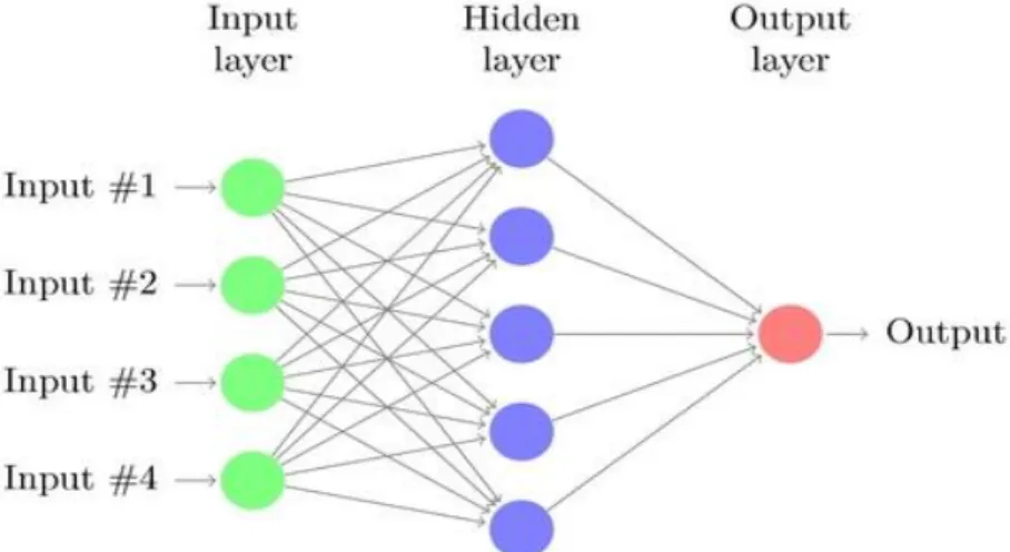
An Artificial Neural Network (ANN) is a computational method that mimics the learning processes of the human brain. This method is inspired by the biological concept of neurons where animals are able to react with their environment (external or internal) using their nervous system. A good artificial model is the one that is capable to simulate the nervous system and response in a similar way. The structure of a neural network consists of input and output and by the learned knowledge that the system tries to map between them (Haykin, 1999).

(19)

The ANN properties are non-linearity and input-output mapping. They can be described as follows (Haykin, 1999):

 Nonlinearity: the ANNs are made of an interconnection of nonlinear neurons.

 Input-Output Mapping: ANNs can use two different learning paradigms:

supervised or unsupervised. Both start with the network assigning weights randomly chosen. Later the learning mechanism starts, in the supervised technique the network is provided by the desired output but the unsupervised techniques let the network responsible for making sense of the input without any help:

a. Supervised training: the input/output are both provided, the network then starts to process the inputs and compares its results against the outputs. Resulting errors are propagated back through the system for adjustment. The process repeatedly occurs as the weights are continually tweaked. In this technique, it is ideal to have enough data so that it can be divided to different sets [training, testing] for monitoring if the network is perfectly learning well. Usually, if the result is not sufficient, the design of the network [number of layers, input, output, the neurons, transfer function and training function] should be modified.

b. Unsupervised, or Adaptive Training: in this case the network is provided by inputs only. Later the system decide which features will use to group the input sample, this is called self-organizing (SO) or adaption. In this sense, adaption means to continually learn on their own as new variables or situations are encountered.

Figure 2 presents the architecture of a simple neural network.

(20)

2.2. RELATED WORK

Prior to analyze the energy use inside the campus, a review of previous work to identify the influence factors and identifying patterns in buildings was necessary. The university campus is considered as a mixed use buildings environment which varies between offices, educational and even residential and commercial. Several researches relied on data analysis methods for getting useful information and knowledge from measured data by following different methodologies (Olofsson et al., 2009; Djurica and Novakovicb, 2012).

The previous researches have contributed to the identification process of a set of factors which are very likely to influence consumption. It is difficult to say that these factors are general since energy consumption depends on many criteria for building's location and environments. However, some of them will be considered as candidates through the analysis process trying to prove the hypothesis of the thesis. The next step after finding the derived factors for the consumption is the use of those factors to predict the energy using two different approaches.

A search of literature reveals that different methods were adopted to develop factors which influence energy consumption such as Regression Analysis and Neural Network. Both are described in the next sections.

2.2.1 R

EGRESSION

A

NALYSIS

Regression analysis is a type of statistical analysis which is widely used in building engineering for spotting the correlation between building energy consumption and its influencing factors like occupancy patterns, building envelope characteristics and heating, ventilation, air-conditioning load (HVAC) system. This technique is also used to analyze overall buildings using patterns and how these factors affect energy consumption.

Corgnati et al. (2008) has performed an analysis of 120 schools in Italy to assess the heating consumption. They collected data from meters that were deployed in schools and organized the data in index mechanism. A normalization among all data was performed, followed by statistics analyses. They collected data about climatic zones, building characteristics and monthly consumption, later a regression method was used to find the relation between the heating consumption and the change in the temperature by seasons (heating degree days and cooling degree days).

(21)

Zmeureanu and Fazio (1991) performed regression analysis of 68 office buildings data collected. One of the conclusions is that buildings’ age has an effect on consumption. Djurica and Novakovicb (2012) also performed principle component regression analysis (PCR) and Partial least square regression on low energy office buildings using data that include occupancy level, inside temperature, water and control signals. They tried to find the correlation between those variables and heating, electricity and fan energy use. The result varies depending on the months. For example, the heating is influenced by the occupancy level operation parameter and not by the outside temperature, whereas the electricity use is influenced by the indoor temperature and occupancy level. Additionally, it was found that the regression model should be updated on monthly basis according to the seasonality change.

Regarding prediction of building energy, regression analysis was widely used, not only to predict energy consumption but also for different factors inside the buildings like occupancy rate and indoor temperature. Lam et al. (1997) modelled high-rise air conditioned office buildings in Hong Kong. They collected data and found that 28 parameters are correlated with the building load and HVAC system. Both linear and non-linear multiple regression techniques were applied to develop a prediction model for annual energy. A number of those parameters were eliminated and only 12 showed high sensitive coefficient to the annual energy use prediction.

Caldera et al. (2008) used statistical analysis for energy demand assessment. Data were collected for 50 buildings with different construction years, trying to correlate the building geometry and thermo-physical parameters, like the volume and the shape, the construction criteria, like glazed surfaces, and the environmental factors, like temperature.

Catalina et al. (2008) undertook a research for developing a regression model to predict monthly heating demand. The model was based on data collected from 16 cities in France. Data comprised buildings envelop characteristics and buildings’ specifications like the construction year, windows and floors area and climate data. The analysis showed that there is a strong relation between the building shape and the consumption. Also, the internal thermal characteristics have a strong effect on consumption. The resulting model was efficient with a maximum deviation between the simulated data of 1.2-5.2 %.

2.2.2 A

RTIFICIAL

N

EURAL NETWORK

In their experiment, Datta et al. (2000) used ANN to predict the electricity demand in a supermarket, in order to control the load and avoid any penalty due to the exceeding of contract's load rate. They made the experiment with half an hour rate, considering the time of the day as one factor in addition to the environmental factors. Using the feed-forward network and training the model with real data from the store, they tested 7 networks with different combinations of input variables such as Day, Time, External Humidity and Temperature, Internal Humidity and Temperature. The results indicated that using a short-term data set may be adequate to accurately predict half hourly electrical demand.

(22)

temperature, wet bulb temperature, dew point temperature, relative humidity percentage, wind speed and wind direction. They were able to successfully predict the chiller plant power consumption depending on meteorological parameters. Ekici and Aksoy (2009) performed a back propagation technique for neural network in order to predict heating energy consumption in buildings with three input and one output values. They trained the network with buildings’ transparency ratio, orientation and insulation thickness. The author mentions that the advantage of using neural network over other methods is its capability of performing complex modeling with high prediction accuracy for heating loads with average of 94.8-98.5%.

With a similar back propagation method, Kalogirou and Bojic (2000) used ANN to predict the energy consumption in passive solar buildings. Several use cases were simulated, depending on variables such as walls insulation and seasons. The network was trained using those variables as input and the consumption as an output. The neural network was successfully used to model the thermal behavior, having a R value of 0.9991. The advantage of the neural model is the adaptation to new input values which were not in the same training set. The authors also revealed as another advantage of using the neural network the fact of its acceptable accuracy in prediction, instead of using other expensive modeling programs for passive solar buildings.

(23)

Chapter Three: STUDY AREA AND DATA

This chapter contains a detailed description of the university and its facilities with the major conservation measurement, which has been done to decrease our carbon footprint. It also includes the description of the data that has been collected and stored.

3.1 THE ROLE OF THE UNIVERSITY IN SUSTAINABILITY

The University Jaume I (UJI) has followed several ways towards sustainability enhancement in the campus, considering the fact that it is composed of a group of diverse buildings with significantly high consumption, representing a small city with different buildings' use (offices, cafeterias, shops, laboratories, sport centre, classrooms, etc.). Therefore, the call for promoting energy sustainability and conservation measurement has been guided in a number of agreements and declarations in Europe, and it has been followed to some extent in the university. The work was promoted on different scales such as the academic programs, which is taught through courses like environmental studies or by rising the awareness through data provision using the university website. Bearing in mind that all higher institutions can affect many teachers, students, leaders and decision makers of tomorrow either in class room or in community work, the green model of the university can be later extended to community scale.

All the work conducted by educational institutions in this area is being recognized, encouraged and funded by the European Union, governments and councils11.

3.2 UNIVERSITY CAMPUS

The University Riu Sec campus is composed of several buildings and with a total built area of 219257.69 m2 12. Depending on their purpose, building types are: administrative, educational, laboratory, and workshop, residential and sport facilities. Figure 3 categorizes all university's buildings.

11

http://www.eeef.eu/

12

(24)

Figure 3: Categories of university buildings

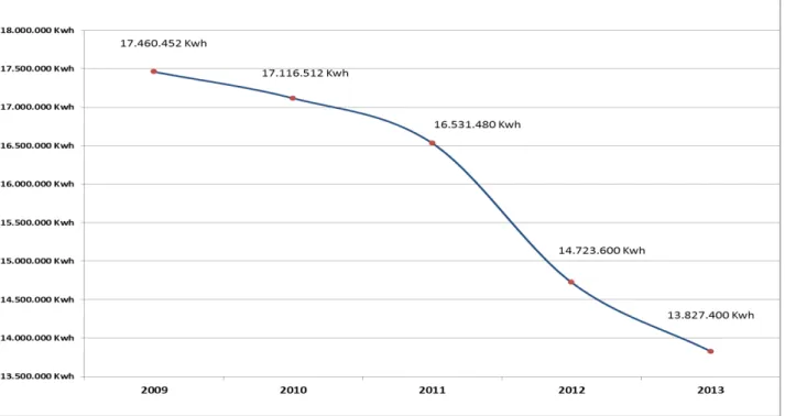
The university took some actions to reduce the energy usage in the campus, as follows:

 Replacement of inefficient cooling/heating machinery;  Installation of photovoltaic system;

 Installation of sensors inside classrooms for "light" and "air conditioning” control;

 Strict control of temperature in classrooms;  Reduction of air conditioning schedules;

 Lighting control schedules (interior and exterior).

(25)

Figure 4: UJI's Energy consumption between 2009 and 2013

In addition to all these measures, an analysis of energy use in the university is highly recommended with further use of ICT (Information and Communication Technologies) in energy monitoring and information provision in campus. The first step was adopted by the management by deploying a system for energy monitoring. The next step will be analyzing those data.

3.3 DATA DESCRIPTION AND COLLECTION

For the purpose of the thesis we needed to collect data for the analysis and modeling from different sources. Data comprise the following:

 Data for energy consumption (historical data);  Data for building specifications (area, type);

 Data for the historical (temperature, humidity, wind speed) measurements;  Data about building occupancy (classes’ schedule) and university calendar.

3.3.1 D

ATA

S

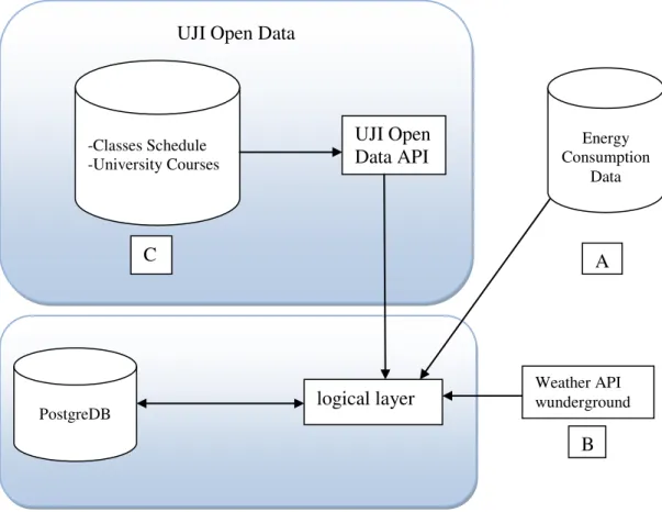
OURCE

(26)

UJI Open Data

Figure 5: Diagram for data sources for analysis and collection process.

Figure 5 comprises 3 groups of data, A, B and C, described as follows.

3.3.1.1 Energy Consumption Data

Set A is composed of the energy consumption data that are collected during the monitoring of the consumption in university using the smart meters which are deployed in several buildings. The smart meter is recording the consumption of energy in different interval scales, and it communicates this information to the utility in two-way communication channel. Smart meters usually include real-time or near real-time sensors, in this case the interval is 15 minutes. The data are then stored in MongoDB.

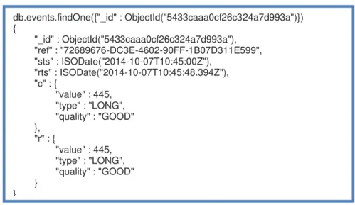
MongoDB13 is a document-oriented database classified as NoSQL. It has a different format called BSON14 (Binary JavaScript Object Notation). Each record in this database is stored as a document, the document schema is similar to JSON15 (JavaScript Object Notation) style objects. Figure 6 illustrates an example of one event document that holds one of the meters' readings, it is composed of field-and-value pairs and has the following structure.

13

https://www.mongodb.org/

14

http://bsonspec.org/

-Classes Schedule -University Courses

Energy Consumption

Data

logical layer Weather API _wunderground UJI Open

Data API Service

A

B C

(27)

Figure 6: Example of one document for one meter reading

This example of document includes the measured value of energy consumption and related sensor data on a specific timestamp for one meter.

Because this system is a new one, this Database does not include any of the historic data. Since we wanted to collect a long duration of data for analysis. Thus the historic data for the duration prior to the new metering system installation were provided by the university's management in Excel sheets format. These Excel data are saved later in PostgreDB. The new system MongoDB is only used in the new developed tool for real time energy visualization, the communication between the monitoring system and the new developed web application was facilitated by developing a Java program.

Previous to analysis, a preprocessing step was applied on these data, in order to remove any outlier and filling the missing data by interpolation method.

3.3.1.2 Environmental Data

Data for historic outside temperature, humidity and wind-speed were collected from

Wunderground API16 (Application Programming Interface) for one year (2014). This

API is providing current and historic weather information with different data format, whereas data observations are every 30 minutes. For collecting these data and saving it in PostgreDB we had to develop a Java program. The data format was in JSON-style, Figure 7 below is a sample of one observation:

16

http://www.wunderground.com/weather/api/

db.events.findOne({"_id" : ObjectId("5433caaa0cf26c324a7d993a")}) {

"_id" : ObjectId("5433caaa0cf26c324a7d993a"), "ref" : "72689676-DC3E-4602-90FF-1B07D311E599", "sts" : ISODate("2014-10-07T10:45:00Z"),

"rts" : ISODate("2014-10-07T10:45:48.394Z"), "c" : {

"value" : 445, "type" : "LONG", "quality" : "GOOD" },

"r" : {

"value" : 445, "type" : "LONG", "quality" : "GOOD" }

(28)

Figure 7: Example of API Weather data in JSON format

3.3.1.3 Building Occupancy Data

Set C is an open data platform provided by the university to users through an RESTful Service, it contains data for academic teachers guide, classes schedule and courses information. This API allows data retrieving in different format such as JSON, RDF, TURTLE and CSV.

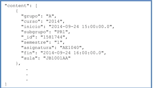
The data for classes schedule were collected and saved in PostgreDB also using developed Java program. This program retrieves all courses and locations where these courses are running with their start and end time. Figure 8 shows a sample of collected data in JSON format.

Figure 8: Sample of classes schedule data provided by UJI Service "observations": [

{

"date": {

"pretty": "1:00 AM CEST on October 02, 2014", "year": "2014", "mon": "10", "mday": "02", "hour": "00", "min": "00", "tzname": "Europe/Madrid" }, "tempm": "19.0", "tempi": "66.2", "dewptm": "18.0", "dewpti": "64.4", "hum": "94", "wspdm": "3.7", "wspdi": "2.3", . . }] "content": [ { "grupo": "A", "curso": "2014",

"inicio": "2014-09-24 15:00:00.0", "subgrupo": "PR1",

"_id": "1581744", "semestre": "1",

"asignatura": "AE1040",

(29)

1.3.1.4 Building Specifications Data

The data regarding the buildings were collected from the university website17, and contain each building surface and floor area. Since the consumption per area is considered one of the important key performance indicators, those data are very important in order to visualize the building efficiency. These data were stored in the campus Geodatabase. The UJI Geodatabase contains geographic layers and stand alone tables for all campus buildings, interior spaces, points of interest (parking areas, waste containers, restaurants and shops, etc.) (Benedito-Bordinau et al., 2013).

3.4 DATA LIMITATION AND ISSUES

During the collection and analysis of the data, we observed some limitations and issues that may cause some impact in the work. Thus, we considered important to list them as follows. We also present some of the solutions we adopted in order to overcome those issues.

1. The monitoring system changed several times and that caused loss of data for the durations between installing each system and the other.

2. Another reason for missing data was the meters malfunction; in order to overcome this fact, we had to use interpolation method to fill the missing data. 3. Some meters are covering a wide area which could include two or three

buildings; that fact makes the analysis difficult as the buildings operation is different in the campus. If there were more meters, the energy tracking and assessment for individual buildings would be improved, this case was not included in the analysis.

4. The meters exact locations is not known, so we had to map the meters by its covered area (building) in a Geographic Information System (GIS). In this case each meter's ID was associated to one building. This step was important for the implementation of the visualization web application.

5. During the past years, meters have been continuously installed, giving a difference in data temporal resolution. Some buildings have measured data starting from 2012 and some from 2014. Data used in the present study only comprise a year from all the collected data (2014).

6. As one of the thesis goal is to gather all possible data about buildings and building's events for more analysis and assessment in the future, the data collection from different resources with different format, as explained in the previous section, consumed a lot of time.

7. Unfortunately, data for the building's envelope, like the thermal

characteristics, were not available, thus we could not take into account those variables in the analysis.

17

(30)

Chapter Four: DATA ANALYSIS

In this chapter, we analyze the collected data to find out if there is any waste in the energy besides investigating the influence factors on the consumption. Later, we use these factors to predict the energy consumption. As an initial step, an exploratory analysis is done in order to give more insight to the data.

4.1. EXPLORATORY DATA ANALYSIS

Behrens (1997) has described the exploratory data analysis (EDA) as a tradition way in data analysis that stems from John Tukey's early work in 1960s (Tukey, 1969). Exploratory analysis can be characterized as:

 An understanding of the data that answer back this main question “What is going on here?"; and

 An emphasis on graphic representations of the data.

Consequently, in addition to the goal of describing of what is going on, a pattern discovery is also revealed by this analysis. Behrens (1997) mentioned that EDA often linked to detective work, as the role of the data analyst is to listen to the data in as many ways as possible until a plausible story of the data is apparent. EDA has many approaches for graphical representation, such as scatter plot, frequency distribution, histogram plot, etc.

In order to make the analysis more efficient, we classified the campus buildings in three main categories according to their main use and operational hours:

1. Classes/Teaching buildings.

2. Administration/companies buildings. 3. Facilities buildings.

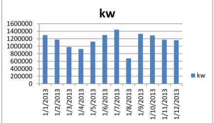
Figure 9 represents the total consumption during the year. Analyzing the general pattern in the university, it is noted one month off-peak, August, when the university is closed, and another peak in September due to the beginning of the semester.

Figure 9: Total energy consumption per month for year 2013

0 200000 400000 600000 800000 1000000 1200000 1400000 1600000

1/1/2013 1/2/2013 1/3/2013 1/4/2013 1/5/2013 1/6/2013 1/7/2013 1/8/2013 1/9/2013 _1/10/2013 _1/11/2013 _1/12/2013

kw

(31)

Due to the limitations of the data that were mentioned before in chapter 3, we will analyze one building that has data available for one year, 2014. The chosen building is the Faculty of Humanities and Social Sciences, which belongs to the category of ' classes/teaching buildings'. The main activities occur during the official academic semester, and the building contains classrooms ('Aula'), laboratories and teacher's offices. The one year data set was divided to two sub data sets, from November to March and from April to October. As the period from November to march has different energy consumption source, the university is using Gas for heating and this source of data is not available. Therefore, this period was excluded from the analysis.

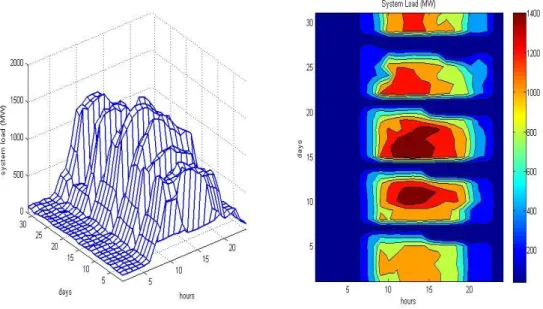
Figure 10 shows the intensity of the consumption of ‘October’. As an example we could notice the pattern which is related to the hour of the day, the consumption starts to increase around 8:00 AM and starts to drop down around 8:00 PM. This pattern is due to the regular operation time and building type, the classes operate from 8:00 AM till 8:00 PM. From the same graph we could see the deviation between the week day and the weekend days.

Figure 10: 3D model for energy load of 'October' 2014, Faculty of Humanities and Social Sciences.

4.1.1 E

NERGY USE PROFILE FOR BUILDINGS

Graphs that presented in next two figures can show how much energy is being used every hour of the day and also for every day in the week, revealing a typical consumption which could be useful for finding energy waste. The small interval details of the measured data could lead to the discovery of any wasting of energy, which can be seen as an advantage. The main important thing is to be able to relate this waste of energy to the activity inside the building or the operation time.

(32)

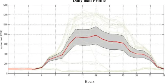
the campus behavior during the day/week, we analyzed the typical hourly consumption for a whole day. In addition to the monthly profile, a standard deviation function was calculated with mean and 95% confidence interval of the daily profile (Figure 11).

Figure 11: Daily Energy Profile of 'October' 2014, Faculty of Humanities and Social Sciences.

As stated before, the data interval makes possible to discover the pattern in energy use. The building has a broad peak, lasting from 11:00 AM to 6:00 PM approximately, during working days. The load is relatively flat at night and early morning, with an increase starting around 6:00 AM. The night-time loads drop at their minimum around midnight. The level of activity on campus is relatively low at night, yet the electricity energy is still high after 8 pm. There are certainly loads at night that cannot be avoided, but this night load can present opportunity for savings, for example reduction of lightening, use of different energy suppliers that are more efficient and also considering power saving in personal computers.

Daily load Profile

Monthly load Profile (Mean, CI) Hours

(33)

The monthly profile (Figure 12) clearly shows the pattern during the working days and the weekend, the same discussed pattern for daily profile is repeated during the working days and the peak drop down sharply during the weekend.

From the two profiles, we could notice that the hour of the day and the day type of the week have an effect on the consumption. Generally, the operation time factor is one of the main drivers for the daily pattern. The consumption for each building during the night is almost the same. We can assume that this residual value is used for the operating machines at night, in the laboratories and servers' rooms.

4.1.2 A

NALYSIS OF CONSUMPTION REGARDING ENVIRONMENTAL FACTORS

We also collected data about the outside temperature and humidity level with the wind speed since we wanted to investigate the relation between the consumption and the outside environmental factors.

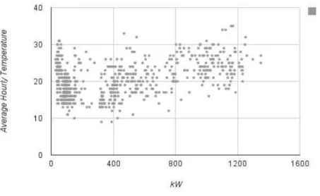
Figure 13: Correlation between hourly consumption (kW) and average hourly temperature for 'October' 2014

(34)

Figure 14: Correlation between hourly consumption (kW) and average hourly humidity for 'October' 2014

Figure 14 shows a negative correlation between the consumption and humidity as R = -0.589. This negative correlation indicates that the consumption is increasing when humidity level is decreasing. From the previous two figures, we can conclude that generally the outside environmental factors could be consider to have some effect on the energy consumption (Table 1).

Factor Correlation coefficient R

Temperature 0.59

Humidity -0.589

Table 1: Environmental factors correlation coefficient for 'October' 2014

4.1.3 R

ELATION BETWEEN THE ENERGY USE AND THE OCCUPANCY LEVEL

(35)

Figure 15: Correlation between classes type (laboratories) and the consumption (kW)

Figure 16: Correlation between classes type (Aula) and the consumption (kW)

(36)

Figure 18: Correlation between day type and the consumption (kW)

Table 2 shows the correlation coefficients from the four occupancy level factors. From the four analyzed factors, it is important to note that the higher correlation is provided by the day type (0.726) and the lowest one is the class type ‘Seminar’ (0.248).

Factor Correlation coefficient R

Class type 'Aula' 0.658

Class type 'Laboratory' 0.681

Class type 'Seminar' 0.248

Day type 0.726

Table 2: Occupancy level factors correlation coefficient

4.2. ENERGY MODELING

There are many factors that have a relation to the high energy consumption. The following goal is to know which one of them could be used as a predictor to build our prediction model. Several techniques can be used in order to build a prediction model. Generally, these models can be divided into two main categories: regression models and ANN models. Both models were built. Their description is presented in the following sections.

4.2.1 S

TEPWISE

R

EGRESSION

(37)

predictors with high correlation. When no additional values exist which could add meaningful statistical relation to the dependent variable, the analysis stops, leaving the variables with low significance outside the equation.

From the above analysis, different independent variables can be used as a predictor for the consumption model.

For better modeling, we need to find the most significant factors among all of these independent variables. In this case, a stepwise regression technique was performed using the following factors:

 Outside temperature;

 Humidity;

 Wind speed;

 Number of classes;

 Number of Seminars;

 Number of laboratories; and

 Day Type [vacation, weekend, weekday].

The analysis was performed by statistical software SPSS. The dependent variable is the energy consumption (kW). It is important to mention that the data are normally distributed and it fit the condition for regression analysis. Table 3 shows the parameters that were entered to the model.

4.2.1.1 Stepwise Multiple Regression for the duration from April to October

Model Variables Entered

Variables Removed

Method

1 Humidity Stepwise (Criteria:

Probability-of-F-to-enter <= .050, Probability-of-F-to-remove >= .100).

2 Aula Stepwise (Criteria:

3 Temperature Stepwise (Criteria:

4 _{Day Type} Stepwise (Criteria:

5 Laboratory Stepwise (Criteria:

6 Wind speed Stepwise (Criteria:

Dependent Variable: kW

(38)

A stepwise multiple regression was conducted to evaluate whether all the variables were necessary to predict the consumption. The stepwise regression works by entering each variable at a time. Variables that entered into the model can be removed at a later step if they are no longer contributing a statistically significant amount of prediction. Each step results in a model, and each successive step modifies the older model and replaces it with a newer one. Each model is tested for statistical significance. The

variable for classes’ type ‘Seminar’ was excluded from the analysis as it shows lower

correlation with the consumption for this duration.

a. Dependent Variable : kW b. Predictors : (constant) , humidity c. Predictors : (constant) , humidity , Aula d. Predictors : (constant) , humidity , Aula , temp

e. Predictors : (constant) , humidity , Aula , temp , Day Type

f. Predictors : (constant) , humidity , Aula , temp , Day Type , Laboratory g. Predictors : (constant) , humidity , Aula , temp , Day Type , Laboratory , wind

Table 4: ANOVA (Analysis of variance) for all 6 predictors

The 6 Analyses of Variance (ANOVA) that are presented in Table 4 correspond to the 6 models. Examining the last column of the output shown in Table 4, it is noteworthy that the final model was built in total six steps; each step resulted in a statistically significant model.

(39)

Finally we conclude from Table 4 that, by using the 6 variables together in the model, we will get the lowest mean square. This result indicates that all those 6 variables significantly influence the dependent variable (Energy consumption - kW). Therefore, it is recommended to use this combination of predictors to predict the consumption. Table 5 presents the model summary which gives details of the overall correlation between the variables left in the model and the dependent variable (kW).

a. Predictors : (constant) , humidity b. Predictors : (constant) , humidity , Aula c. Predictors : (constant) , humidity , Aula , temp

d. Predictors : (constant) , humidity , Aula , temp , Day Type

e. Predictors : (constant) , humidity , Aula , temp , Day Type , Laboratory f. Predictors : (constant) , humidity , Aula , temp , Day Type , Laboratory , wind g. Dependent Variable : kW

Table 5: Model summary for R and R Square values

Table 5 shows the model summary with values of correlation coefficient and coefficient of determination for all the models that were created during the whole process of stepwise regression. This table presents the R Square and adjusted R Square values for each step.

By examining Table 5, we can see in the footnote that humidity variable was entered into the model and the resulted R Square was (0.088). Next step, when Aula variable entered the model the R Square with both predictors has increased to (0.130) with gained value for R Square of (0.042). We can notice that R Square changed from one step to another and by the time we arrived to the last step, the R Square has value of (0.185).

(40)

Table 6: Coefficient table for all models built on combination of the six predictors.

Table 6 provides the results of the calculated coefficients. It is important to note that the standardized regression coefficients are readjusted at each step to reflect the additional variables in the model. The table shows the linear regression equation coefficients for the various model variables. From those coefficient values, a prediction equation can be easily derived for each model. Model 6 comprises all the predictors’ values entered to the stepwise model."B" values are the coefficients for each variable, i.e., they are the value which the variable's data should be multiplied by in the final linear equation. "Constant" is the equivalent interception in the equation. The Significance (“Sig.” in Table 6) values should be 0.05 or below to be significant at 95 percent. A value of 0.000 means the value is too small for three decimal place representation.

The prediction equation should be presented as follows (Eq. 2):

y = constant + (v1 x coeff1) + (v2 x coeff2) + ...)………..Eq. 2

For the studied prediction model, Eq. 2 can be written as follows:

Predicted kW = 111.131 + (-3.631 humidity + 44.497 aula + 14.809 temp + 131.229 day type + (-45.551 laboratory) + (-2.935 wind)).

(41)

of kW (R Square = 0.185, Adjusted R Square = 0.184). The consumption variable kW was primarily predicted by Humidity, and to a lesser extent by higher levels of Aula (classrooms), Temperature, Day type, Laboratory and Wind speed.

The standardized regression coefficients of the predictors together with their correlations with kW (Table 6) shows Humidity received the strongest weight in the model followed by Aula and Temperature.

4.2.1.2 Regression for each month

In order to understand the influencing factors for each month of the year, the same previous steps were applied separately for the study period, between April and October. Factors vary between each month (Tables 7 to 13; Figures 19 to 25, respectively to months April to October).

a. month= 4

b. Predictors: (constant), Aula

c. Predictors: (constant), Aula, Day Type d. Dependent Variable: kW

Table 7: (April) Model summary for R and R Square values for each independent variable.

As described before in the previous section, Table 7 indicates that, for the duration of month April, the most significant predictors are Aula and Day type. Examining this table we can see that Aula variable was entered into the model and the resulted R Square was (0.433). Next step when Day type variable entered the model, the R Square with both predictors has increased to (0.527) and the estimated standard error decreased.

We can conclude that for month April, these are the most significant predictors with a model percentage reach to approximately 53% of the variance of kW.

The ANOVA, Coefficients and excluded variables tables for month April are depicted in Appendixes A.

(42)

Figure 19: (April) Correlation between classes type (Aula), day type and the consumption (kW)

It is noted that the environmental factors are not significantly affecting the consumption during this month, and only factors related with occupancy are highly affecting the energy consumption. This could be due to the moderate temperature at this month.

Table 8 presents the model summary for the month of May.

a. month= 5

b. Predictors: (constant), Aula c. Predictors: (constant), Aula, temp

d. Predictors: (constant), Aula, temp, Day Type e. Predictors: (constant), Aula, temp, Day Type, wind f. Predictors: (constant), Aula, temp, Day Type, Seminar g. Dependent Variable: kW

Table 8: (May) Model summary for R and R Square values for each independent variable.

For May, four predictors are more significant than the rest of variables. These variables are Aula, Temperature, Day Type, Seminar. The lowest standard error and the highest R Square is defined by the combination of the 4 factors together (0.420). We can say that these variables are contains 42% of variance of kW (dependent variable). It also noticed that Class type Seminar has effect on the consumption at this month only.

In Appendix B ANOVA, Coefficients and excluded variables tables for month May are attached.

(43)

Figure 20 displays the correlation between the dependent variable kW and the predictors for this month Wind, Temperature, Seminar, Aula, Day Type respectively.

(44)

Table 9 portrays the modelling results for the month of June.

a. month= 6

b. Predictors: (constant), temp

c. Predictors: (constant), temp, Day Type d. Predictors: (constant), temp, Day Type, wind

e. Predictors: (constant), temp, Day Type, wind, humidity f. Dependent Variable: kW

Table 9: (June) Model summary for R and R Square values for each independent variable.

In June, the environmental factors are statistically significant: temperature, wind, humidity and day type. This combination of predictors is estimated with 34% of variance of kilowatt. In Appendix C ANOVA, Coefficients and excluded variables tables for month June are attached.

Figure 21 shows respectively the partial plot for the predictors of month of June (temperature, humidity, wind , day type).

Figure 21: (June) Correlation between temp, humidity, wind, day type and the consumption (kW) humidity

temp

Professor, Institute of New Imaging Technologies, Universitat Jaume I, Castellón, Spain Dissertation co-supervised by

Nourhan Khalifa Abdelkareem

Analysis and Visualization of Energy use for University

Campus

ACKNOWLEDGMENTS

ABSTRACT

TABLE OF CONTENTS

TABLE OF FIGURES

TABLE OF TABLES

KEYWORDS

ACRONYMS

Chapter One: INTRODUCTION

1.1.

BACKGROUND

1.2.

PROBLEM STATEMENT

1.3.

OBJECTIVES

1.4.

RESEARCH QUESTION AND HYPOTHESIS

1.5.

GENERAL METHODOLOGY

1.5.1

D

C

1.5.2

E

1.5.3

E

1.5.4

V

1.6.

ORGANIZATION OF THE THESIS

Chapter Two: Theoretical Framework

2.1.

CONCEPTS AND DEFINITIONS

2.1.1

R

2.1.2

A

N

(ANN)

2.2.

RELATED WORK

2.2.1

R

A

2.2.2

A

N

Chapter Three: STUDY AREA AND DATA

3.1

THE ROLE OF THE UNIVERSITY IN SUSTAINABILITY

3.2 UNIVERSITY CAMPUS

3.3

DATA DESCRIPTION AND COLLECTION

3.3.1

D

S

3.4 DATA LIMITATION AND ISSUES

Chapter Four: DATA ANALYSIS

4.1.

EXPLORATORY DATA ANALYSIS

kw

4.1.1

E

4.1.2

A

4.1.3

R

4.2.

ENERGY MODELING

4.2.1

S

R