Editors
S.S. Antman J.E. Marsden L. Sirovich
Geophysics and Planetary Sciences Mathematical Biology
L. Glass,J.D. Murray
Mechanics and Materials R.V. Kohn
Systems and Control
S.S. Sastry,P.S. Krishnaprasad
Problems in engineering, computational science, and the physical and biological sciences are using increasingly sophisticated mathematical techniques. Thus, the bridge between the mathematical sciences and other disciplines is heavily traveled. The correspondingly increased dialog between the disciplines has led to the estab-lishment of the series:Interdisciplinary Applied Mathematics.
The purpose of this series is to meet the current and future needs for the interaction between various science and technology areas on the one hand and mathematics on the other. This is done, firstly, by encouraging the ways that mathematics may be applied in traditional areas, as well as point towards new and innovative areas of applications; and, secondly, by encouraging other scientific disciplines to engage in a dialog with mathematicians outlining their problems to both access new methods and suggest innovative developments within mathematics itself.
1. Gutzwiller: Chaos in Classical and Quantum Mechanics 2. Wiggins: Chaotic Transport in Dynamical Systems 3. Joseph/Renardy: Fundamentals of Two-Fluid Dynamics:
Part I: Mathematical Theory and Applications 4. Joseph/Renardy: Fundamentals of Two-Fluid Dynamics:
Part II: Lubricated Transport, Drops and Miscible Liquids 5.
6. Hornung: Homogenization and Porous Media 7.
8.
9. Han/Reddy: Plasticity: Mathematical Theory and Numerical Analysis 10. Sastry: Nonlinear Systems: Analysis, Stability, and Control
11. McCarthy: Geometric Design of Linkages
12. Winfree: The Geometry of Biological Time (Second Edition)
13. Bleistein/Cohen/Stockwell: Mathematics of Multidimensional Seismic Imaging, Migration, and Inversion
14. Okubo/Levin: Diffusion and Ecological Problems: Modern Perspectives 15. Logan: Transport Models in Hydrogeochemical Systems
16. Torquato: Random Heterogeneous Materials: Microstructure and Macroscopic Properties
17. Murray: Mathematical Biology: An Introduction
18. Murray: Mathematical Biology: Spatial Models and Biomedical Applications
19. Kimmel/Axelrod: Branching Processes in Biology 20. Fall/Marland/Wagner/Tyson: Computational Cell Biology
21. Schlick: Molecular Modeling and Simulation: An Interdisciplinary Guide 22. Sahimi: Heterogenous Materials: Linear Transport and Optical Properties
(Volume I)
23. Sahimi: Heterogenous Materials: Non-linear and Breakdown Properties and Atomistic Modeling (Volume II)
24. Bloch: Nonhoionomic Mechanics and Control
25. Beuter/Glass/Mackey/Titcombe: Nonlinear Dynamics in Physiology and Medicine
26. Ma/Soatto/Kosecka/Sastry: An invitation to 3-D Vision 27. Ewens: Mathematical Population Genetics (Second Edition) 28. Wyatt: Quantum Dynamics with Trajectories
29. Karniadakis: Microflows and Nanoflows
30. Macheras: Modeling in Biopharmaceutics, Pharmacokinetics and Pharmacodynamics
31. Samelson/Wiggins: Lagrangian Transport in Geophysical Jets and Waves 32. Wodarz: Killer Cell Dynamics
33. Pettini: Geometry and Topology in Hamiltonian Dynamics and Statistical Mechanics
34. Desolneux/Moisan/Morel: From Gestalt Theory to Image Analysis
Keener/Sneyd: Mathematical Physiology, Second Edition: From Equilibrium to Chaos
Seydel: Practical Bifurcation and Stability Analysis:
II: Systems Physiology
Mathematical Physiology
I: Cellular Physiology
Second Edition
Series Editors
S.S. Antman J.E. Marsden
Department of Mathematics and Control and Dynamical Systems Institute for Physical Science and Mail Code 107-81
Technology
University of Maryland Pasadena, CA 91125 College Park, MD 20742 USA
L. Sirovich
Laboratory of Applied Mathematics Department of Biomathematics Mt. Sinai School of Medicine Box 1012
NYC 10029 USA
All rights reserved. This work may not be translated or copied in whole or in part without the written permission of the publisher (Springer Science+Business Media, LLC, 233 Spring Street, New York, NY 10013, USA), except for brief excerpts in connection with reviews or scholarly analysis. Use in connection with any form of information storage and retrieval, electronic adaptation, computer software, or by similar or dissimilar methodology now known or hereafter developed is forbidden.
The use in this publication of trade names, trademarks, service marks, and similar terms, even if they are not identified as such, is not to be taken as an expression of opinion as to whether or not they are subject to proprietary rights.
springer.com
Salt Lake City, 84112 USA
[email protected] University of Utah
ISBN 978-0-387-75846-6 e-ISBN 978-0-387-75847-3
Library of Congress Control Number: 2008931057
Printed on acid-free paper. DOI 10.1007/978-0-387-75847-3
[email protected] Auckland, New Zealand
California Institute of Technology Private Bag 92019
and
If, in 1998, it was presumptuous to attempt to summarize the field of mathematical physiology in a single book, it is even more so now. In the last ten years, the number of applications of mathematics to physiology has grown enormously, so that the field, large then, is now completely beyond the reach of two people, no matter how many volumes they might write.
Nevertheless, although the bulk of the field can be addressed only briefly, there are certain fundamental models on which stands a great deal of subsequent work. We believe strongly that a prerequisite for understanding modern work in mathematical physiology is an understanding of these basic models, and thus books such as this one serve a useful purpose.
With this second edition we had two major goals. The first was to expand our discussion of many of the fundamental models and principles. For example, the con-nection between Gibbs free energy, the equilibrium constant, and kinetic rate theory is now discussed briefly, Markov models of ion exchangers and ATPase pumps are dis-cussed at greater length, and agonist-controlled ion channels make an appearance. We also now include some of the older models of fluid transport, respiration/perfusion, blood diseases, molecular motors, smooth muscle, neuroendocrine cells, the barore-ceptor loop, tubuloglomerular oscillations, blood clotting, and the retina. In addition, we have expanded our discussion of stochastic processes to include an introduction to Markov models, the Fokker–Planck equation, the Langevin equation, and applications to such things as diffusion, and single-channel data.
extensive. Nevertheless, we hope that in each chapter, enough information is given to enable the interested reader to pursue the topic further.
Of course, our survey has unavoidable omissions, some intentional, others not. We can only apologize, yet again, for these, and beg the reader’s indulgence. As with the first edition, ignorance and exhaustion are the cause, although not the excuse.
Since the publication of the first edition, we have received many comments (some even polite) about mistakes and omissions, and a number of people have devoted con-siderable amounts of time to help us improve the book. Our particular thanks are due to Richard Bertram, Robin Callard, Erol Cerasi, Martin Falcke, Russ Hamer, Harold Layton, Ian Parker, Les Satin, Jim Selgrade and John Tyson, all of whom assisted above and beyond the call of duty. We also thank Peter Bates, Dan Beard, Andrea Ciliberto, Silvina Ponce Dawson, Charles Doering, Elan Gin, Erin Higgins, Peter Jung, Yue Xian Li, Mike Mackey, Robert Miura, Kim Montgomery, Bela Novak, Sasha Panfilov, Ed Pate, Antonio Politi, Tilak Ratnanather, Timothy Secomb, Eduardo Sontag, Mike Steel, and Wilbert van Meerwijk for their help and comments.
Finally, we thank the University of Auckland and the University of Utah for contin-uing to pay our salaries while we devoted large fractions of our time to writing, and we thank the Royal Society of New Zealand for the James Cook Fellowship to James Sneyd that has made it possible to complete this book in a reasonable time.
University of Utah James Keener
University of Auckland James Sneyd
It can be argued that of all the biological sciences, physiology is the one in which mathematics has played the greatest role. From the work of Helmholtz and Frank in the last century through to that of Hodgkin, Huxley, and many others in this century, physiologists have repeatedly used mathematical methods and models to help their understanding of physiological processes. It might thus be expected that a close con-nection between applied mathematics and physiology would have developed naturally, but unfortunately, until recently, such has not been the case.
There are always barriers to communication between disciplines. Despite the quantitative nature of their subject, many physiologists seek only verbal descriptions, naming and learning the functions of an incredibly complicated array of components; often the complexity of the problem appears to preclude a mathematical description. Others want to become physicians, and so have little time for mathematics other than to learn about drug dosages, office accounting practices, and malpractice liability. Still others choose to study physiology precisely because thereby they hope not to study more mathematics, and that in itself is a significant benefit. On the other hand, many applied mathematicians are concerned with theoretical results, proving theorems and such, and prefer not to pay attention to real data or the applications of their results. Others hesitate to jump into a new discipline, with all its required background reading and its own history of modeling that must be learned.
Halley’s comet will return. Your head will be full of interesting and important facts, but it is difficult to organize those facts unless they are given a quantitative description. Similarly, if applied mathematicians were to ignore physiology, they would be losing the opportunity to study an extremely rich and interesting field of science.
To explain the goals of this book, it is most convenient to begin by emphasizing what this book is not; it is not a physiology book, and neither is it a mathematics book. Any reader who is seriously interested in learning physiology would be well advised to consult an introductory physiology book such as Guyton and Hall (1996) or Berne and Levy (1993), as, indeed, we ourselves have done many times. We give only a brief background for each physiological problem we discuss, certainly not enough to satisfy a real physiologist. Neither is this a book for learning mathematics. Of course, a great deal of mathematics is used throughout, but any reader who is not already familiar with the basic techniques would again be well advised to learn the material elsewhere.
Instead, this book describes work that lies on the border between mathematics and physiology; it describes ways in which mathematics may be used to give insight into physiological questions, and how physiological questions can, in turn, lead to new mathematical problems. In this sense, it is truly an interdisciplinary text, which, we hope, will be appreciated by physiologists interested in theoretical approaches to their subject as well as by mathematicians interested in learning new areas of application.
It is also an introductory survey of what a host of other people have done in em-ploying mathematical models to describe physiological processes. It is necessarily brief, incomplete, and outdated (even before it was written), but we hope it will serve as an introduction to, and overview of, some of the most important contributions to the field. Perhaps some of the references will provide a starting point for more in-depth investigations.
Unfortunately, because of the nature of the respective disciplines, applied mathe-maticians who know little physiology will have an easier time with this material than will physiologists with little mathematical training. A complete understanding of all of the mathematics in this book will require a solid undergraduate training in mathe-matics, a fact for which we make no apology. We have made no attempt whatever to water down the models so that a lower level of mathematics could be used, but have instead used whatever mathematics the physiology demands. It would be misleading to imply that physiological modeling uses only trivial mathematics, or vice versa; the essential richness of the field results from the incorporation of complexities from both disciplines.
extensive use of asymptotic methods and perturbation theory, but include explanatory material to help the novice understand the calculations.
This book can be used in several ways. It could be used to teach a full-year course in mathematical physiology, and we have used this material in that way. The book includes enough exercises to keep even the most diligent student busy. It could also be used as a supplement to other applied mathematics, bioengineering, or physiology courses. The models and exercises given here can add considerable interest and challenge to an otherwise traditional course.
The book is divided into two parts, the first dealing with the fundamental principles of cell physiology, and the second with the physiology of systems. After an introduc-tion to basic biochemistry and enzyme reacintroduc-tions, we move on to a discussion of various aspects of cell physiology, including the problem of volume control, the membrane po-tential, ionic flow through channels, and excitability. Chapter 5 is devoted to calcium dynamics, emphasizing the two important ways that calcium is released from stores, while cells that exhibit electrical bursting are the subject of Chapter 6. This book is not intentionally organized around mathematical techniques, but it is a happy coinci-dence that there is no use of partial differential equations throughout these beginning chapters.
Spatial aspects, such as synaptic transmission, gap junctions, the linear cable equa-tion, nonlinear wave propagation in neurons, and calcium waves, are the subject of the next few chapters, and it is here that the reader first meets partial differential equations. The most mathematical sections of the book arise in the discussion of signaling in two-and three-dimensional media—readers who are less mathematically inclined may wish to skip over these sections. This section on basic physiological mechanisms ends with a discussion of the biochemistry of RNA and DNA and the biochemical regulation of cell function.
The second part of the book gives an overview of organ physiology, mostly from the human body, beginning with an introduction to electrocardiology, followed by the physiology of the circulatory system, blood, muscle, hormones, and the kidneys. Finally, we examine the digestive system, the visual system, ending with the inner ear.
As well as noticing the omission of a number of important areas of mathematical physiology, the reader may also notice that our view of what “mathematical” means appears to be somewhat narrow as well. For example, we include very little discussion of statistical methods, stochastic models, or discrete equations, but concentrate almost wholly on continuous, deterministic approaches. We emphasize that this is not from any inherent belief in the superiority of continuous differential equations. It results rather from the unpleasant fact that choices had to be made, and when push came to shove, we chose to include work with which we were most familiar. Again, apologies are offered.
Finally, with a project of this size there is credit to be given and blame to be cast; credit to the many people, like the pioneers in the field whose work we freely bor-rowed, and many reviewers and coworkers (Andrew LeBeau, Matthew Wilkins, Richard Bertram, Lee Segel, Bruce Knight, John Tyson, Eric Cytrunbaum, Eric Marland, Tim Lewis, J.G.T. Sneyd, Craig Marshall) who have given invaluable advice. Particular thanks are also due to the University of Canterbury, New Zealand, where a signifi-cant portion of this book was written. Of course, as authors we accept all the blame for not getting it right, or not doing it better.
University of Utah James Keener
University of Michigan James Sneyd
With a project of this size it is impossible to give adequate acknowledgment to everyone who contributed: My family, whose patience with me is herculean; my students, who had to tolerate my rantings, ravings, and frequent mistakes; my colleagues, from whom I learned so much and often failed to give adequate attribution. Certainly the most profound contribution to this project was from the Creator who made it all possible in the first place. I don’t know how He did it, but it was a truly astounding achievement. To all involved, thanks.
University of Utah James Keener
Between the three of them, Jim Murray, Charlie Peskin and Dan Tranchina have taught me almost everything I know about mathematical physiology. This book could not have been written without them, and I thank them particularly for their, albeit unaware, contributions. Neither could this book have been written without many years of support from my parents and my wife, to whom I owe the greatest of debts.
CONTENTS, I: Cellular Physiology
Preface to the Second Edition vii
Preface to the First Edition ix
Acknowledgments xiii
1 Biochemical Reactions 1
1.1 The Law of Mass Action . . . 1
1.2 Thermodynamics and Rate Constants . . . 3
1.3 Detailed Balance . . . 6
1.4 Enzyme Kinetics . . . 7
1.4.1 The Equilibrium Approximation . . . 8
1.4.2 The Quasi-Steady-State Approximation . . . 9
1.4.3 Enzyme Inhibition . . . 12
1.4.4 Cooperativity . . . 15
1.4.5 Reversible Enzyme Reactions . . . 20
1.4.6 The Goldbeter–Koshland Function . . . 21
1.6 Appendix: Math Background . . . 33
1.6.1 Basic Techniques . . . 35
1.6.2 Asymptotic Analysis . . . 37
1.6.3 Enzyme Kinetics and Singular Perturbation Theory . . . 39
1.7 Exercises . . . 42
2 Cellular Homeostasis 49 2.1 The Cell Membrane . . . 49
2.2 Diffusion . . . 51
2.2.1 Fick’s Law . . . 52
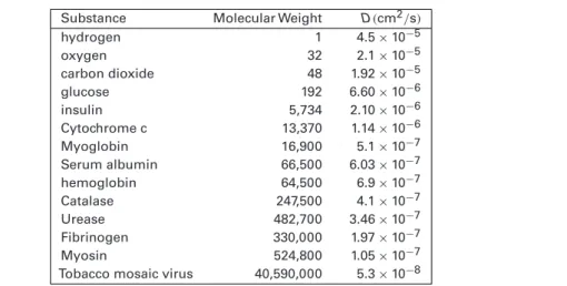
2.2.2 Diffusion Coefficients . . . 53
2.2.3 Diffusion Through a Membrane: Ohm’s Law . . . 54
2.2.4 Diffusion into a Capillary . . . 55
2.2.5 Buffered Diffusion . . . 55
2.3 Facilitated Diffusion . . . 58
2.3.1 Facilitated Diffusion in Muscle Respiration . . . 61
2.4 Carrier-Mediated Transport . . . 63
2.4.1 Glucose Transport . . . 64
2.4.2 Symports and Antiports . . . 67
2.4.3 Sodium–Calcium Exchange . . . 69
2.5 Active Transport . . . 73
2.5.1 A Simple ATPase . . . 74
2.5.2 Active Transport of Charged Ions . . . 76
2.5.3 A Model of the Na+– K+ATPase . . . . 77
2.5.4 Nuclear Transport . . . 79
2.6 The Membrane Potential . . . 80
2.6.1 The Nernst Equilibrium Potential . . . 80
2.6.2 Gibbs–Donnan Equilibrium . . . 82
2.6.3 Electrodiffusion: The Goldman–Hodgkin–Katz Equations . . 83
2.6.4 Electrical Circuit Model of the Cell Membrane . . . 86
2.7 Osmosis . . . 88
2.8 Control of Cell Volume . . . 90
2.8.1 A Pump–Leak Model . . . 91
2.8.2 Volume Regulation and Ionic Transport . . . 98
2.9 Appendix: Stochastic Processes . . . 103
2.9.1 Markov Processes . . . 103
2.9.2 Discrete-State Markov Processes . . . 105
2.9.3 Numerical Simulation of Discrete Markov Processes . . . 107
2.9.4 Diffusion . . . 109
2.9.5 Sample Paths; the Langevin Equation . . . 110
2.9.6 The Fokker–Planck Equation and the Mean First Exit Time . 111 2.9.7 Diffusion and Fick’s Law . . . 114
3 Membrane Ion Channels 121
3.1 Current–Voltage Relations . . . 121
3.1.1 Steady-State and Instantaneous Current–Voltage Relations . 123 3.2 Independence, Saturation, and the Ussing Flux Ratio . . . 125
3.3 Electrodiffusion Models . . . 128
3.3.1 Multi-Ion Flux: The Poisson–Nernst–Planck Equations . . . . 129
3.4 Barrier Models . . . 134
3.4.1 Nonsaturating Barrier Models . . . 136
3.4.2 Saturating Barrier Models: One-Ion Pores . . . 139
3.4.3 Saturating Barrier Models: Multi-Ion Pores . . . 143
3.4.4 Electrogenic Pumps and Exchangers . . . 145
3.5 Channel Gating . . . 147
3.5.1 A Two-State K+Channel . . . 148
3.5.2 Multiple Subunits . . . 149
3.5.3 The Sodium Channel . . . 150
3.5.4 Agonist-Controlled Ion Channels . . . 152
3.5.5 Drugs and Toxins . . . 153
3.6 Single-Channel Analysis . . . 155
3.6.1 Single-Channel Analysis of a Sodium Channel . . . 155
3.6.2 Single-Channel Analysis of an Agonist-Controlled Ion Channel . . . 158
3.6.3 Comparing to Experimental Data . . . 160
3.7 Appendix: Reaction Rates . . . 162
3.7.1 The Boltzmann Distribution . . . 163
3.7.2 A Fokker–Planck Equation Approach . . . 165
3.7.3 Reaction Rates and Kramers’ Result . . . 166
3.8 Exercises . . . 170
4 Passive Electrical Flow in Neurons 175 4.1 The Cable Equation . . . 177
4.2 Dendritic Conduction . . . 180
4.2.1 Boundary Conditions . . . 181
4.2.2 Input Resistance . . . 182
4.2.3 Branching Structures . . . 182
4.2.4 A Dendrite with Synaptic Input . . . 185
4.3 The Rall Model of a Neuron . . . 187
4.3.1 A Semi-Infinite Neuron with a Soma . . . 187
4.3.2 A Finite Neuron and Soma . . . 189
4.3.3 Other Compartmental Models . . . 192
4.4 Appendix: Transform Methods . . . 192
5 Excitability 195
5.1 The Hodgkin–Huxley Model . . . 196
5.1.1 History of the Hodgkin–Huxley Equations . . . 198
5.1.2 Voltage and Time Dependence of Conductances . . . 200
5.1.3 Qualitative Analysis . . . 210
5.2 The FitzHugh–Nagumo Equations . . . 216
5.2.1 The Generalized FitzHugh-Nagumo Equations . . . 219
5.2.2 Phase-Plane Behavior . . . 220
5.3 Exercises . . . 223
6 Wave Propagation in Excitable Systems 229 6.1 Brief Overview of Wave Propagation . . . 229
6.2 Traveling Fronts . . . 231
6.2.1 The Bistable Equation . . . 231
6.2.2 Myelination . . . 236
6.2.3 The Discrete Bistable Equation . . . 238
6.3 Traveling Pulses . . . 242
6.3.1 The FitzHugh–Nagumo Equations . . . 242
6.3.2 The Hodgkin–Huxley Equations . . . 250
6.4 Periodic Wave Trains . . . 252
6.4.1 Piecewise-Linear FitzHugh–Nagumo Equations . . . 253
6.4.2 Singular Perturbation Theory . . . 254
6.4.3 Kinematics . . . 256
6.5 Wave Propagation in Higher Dimensions . . . 257
6.5.1 Propagating Fronts . . . 258
6.5.2 Spatial Patterns and Spiral Waves . . . 262
6.6 Exercises . . . 268
7 Calcium Dynamics 273 7.1 Calcium Oscillations and Waves . . . 276
7.2 Well-Mixed Cell Models: Calcium Oscillations . . . 281
7.2.1 Influx . . . 282
7.2.2 Mitochondria . . . 282
7.2.3 Calcium Buffers . . . 282
7.2.4 Calcium Pumps and Exchangers . . . 283
7.2.5 IP3 Receptors . . . 285
7.2.6 Simple Models of Calcium Dynamics . . . 293
7.2.7 Open- and Closed-Cell Models . . . 296
7.2.8 IP3Dynamics . . . 298
7.2.9 Ryanodine Receptors . . . 301
7.3 Calcium Waves . . . 303
7.3.1 Simulation of Spiral Waves inXenopus . . . 306
7.4 Calcium Buffering . . . 309
7.4.1 Fast Buffers or Excess Buffers . . . 310
7.4.2 The Existence of Buffered Waves . . . 313
7.5 Discrete Calcium Sources . . . 315
7.5.1 The Fire–Diffuse–Fire Model . . . 318
7.6 Calcium Puffs and Stochastic Modeling . . . 321
7.6.1 Stochastic IPR Models . . . 323
7.6.2 Stochastic Models of Calcium Waves . . . 324
7.7 Intercellular Calcium Waves . . . 326
7.7.1 Mechanically Stimulated Intercellular Ca2+Waves . . . 327
7.7.2 Partial Regeneration . . . 330
7.7.3 Coordinated Oscillations in Hepatocytes . . . 331
7.8 Appendix: Mean Field Equations . . . 332
7.8.1 Microdomains . . . 332
7.8.2 Homogenization; Effective Diffusion Coefficients . . . 336
7.8.3 Bidomain Equations . . . 341
7.9 Exercises . . . 341
8 Intercellular Communication 347 8.1 Chemical Synapses . . . 348
8.1.1 Quantal Nature of Synaptic Transmission . . . 349
8.1.2 Presynaptic Voltage-Gated Calcium Channels . . . 352
8.1.3 Presynaptic Calcium Dynamics and Facilitation . . . 358
8.1.4 Neurotransmitter Kinetics . . . 364
8.1.5 The Postsynaptic Membrane Potential . . . 370
8.1.6 Agonist-Controlled Ion Channels . . . 371
8.1.7 Drugs and Toxins . . . 373
8.2 Gap Junctions . . . 373
8.2.1 Effective Diffusion Coefficients . . . 374
8.2.2 Homogenization . . . 376
8.2.3 Measurement of Permeabilities . . . 377
8.2.4 The Role of Gap-Junction Distribution . . . 377
8.3 Exercises . . . 383
9 Neuroendocrine Cells 385 9.1 PancreaticβCells . . . 386
9.1.1 Bursting in the PancreaticβCell . . . 386
9.1.2 ER Calcium as a Slow Controlling Variable . . . 392
9.1.3 Slow Bursting and Glycolysis . . . 399
9.1.4 Bursting in Clusters . . . 403
9.1.5 A Qualitative Bursting Model . . . 410
9.2 Hypothalamic and Pituitary Cells . . . 419
9.2.1 The Gonadotroph . . . 419
9.3 Exercises . . . 424
10 Regulation of Cell Function 427 10.1 Regulation of Gene Expression . . . 428
10.1.1 ThetrpRepressor . . . 429
10.1.2 ThelacOperon . . . 432
10.2 Circadian Clocks . . . 438
10.3 The Cell Cycle . . . 442
10.3.1 A Simple Generic Model . . . 445
10.3.2 Fission Yeast . . . 452
10.3.3 A Limit Cycle Oscillator in theXenopusOocyte . . . 461
10.3.4 Conclusion . . . 468
10.4 Exercises . . . 468
Appendix: Units and Physical Constants A-1 References R-1 Index I-1
CONTENTS, II: Systems Physiology
Preface to the Second Edition vii Preface to the First Edition ix Acknowledgments xiii 11 The Circulatory System 471 11.1 Blood Flow . . . 47311.2 Compliance . . . 476
11.3 The Microcirculation and Filtration . . . 479
11.4 Cardiac Output . . . 482
11.5 Circulation . . . 484
11.5.1 A Simple Circulatory System . . . 484
11.5.2 A Linear Circulatory System . . . 486
11.5.3 A Multicompartment Circulatory System . . . 488
11.6 Cardiovascular Regulation . . . 495
11.6.1 Autoregulation . . . 497
11.6.2 The Baroreceptor Loop . . . 500
11.7 Fetal Circulation . . . 507
11.8 The Arterial Pulse . . . 513
11.8.1 The Conservation Laws . . . 513
11.8.2 The Windkessel Model . . . 514
11.8.3 A Small-Amplitude Pressure Wave . . . 516
11.8.4 Shock Waves in the Aorta . . . 516
11.9 Exercises . . . 521
12 The Heart 523 12.1 The Electrocardiogram . . . 525
12.1.1 The Scalar ECG . . . 525
12.1.2 The Vector ECG . . . 526
12.2 Cardiac Cells . . . 534
12.2.1 Purkinje Fibers . . . 535
12.2.2 Sinoatrial Node . . . 541
12.2.3 Ventricular Cells . . . 543
12.2.4 Cardiac Excitation–Contraction Coupling . . . 546
12.2.5 Common-Pool and Local-Control Models . . . 548
12.2.6 The L-type Ca2+Channel . . . 550
12.2.7 The Ryanodine Receptor . . . 551
12.2.8 The Na+–Ca2+Exchanger . . . 552
12.3 Cellular Coupling . . . 553
12.3.1 One-Dimensional Fibers . . . 554
12.3.2 Propagation Failure . . . 561
12.3.3 Myocardial Tissue: The Bidomain Model . . . 566
12.3.4 Pacemakers . . . 572
12.4 Cardiac Arrhythmias . . . 583
12.4.1 Cellular Arrhythmias . . . 584
12.4.2 Atrioventricular Node—Wenckebach Rhythms . . . 586
12.4.3 Reentrant Arrhythmias . . . 593
12.5 Defibrillation . . . 604
12.5.1 The Direct Stimulus Threshold . . . 608
12.5.2 The Defibrillation Threshold . . . 610
12.6 Appendix: The Sawtooth Potential . . . 613
12.7 Appendix: The Phase Equations . . . 614
12.8 Appendix: The Cardiac Bidomain Equations . . . 618
12.9 Exercises . . . 622
13 Blood 627 13.1 Blood Plasma . . . 628
13.2 Blood Cell Production . . . 630
13.2.1 Periodic Hematological Diseases . . . 632
13.2.2 A Simple Model of Blood Cell Growth . . . 633
13.3 Erythrocytes . . . 643
13.3.1 Myoglobin and Hemoglobin . . . 643
13.3.2 Hemoglobin Saturation Shifts . . . 648
13.3.3 Carbon Dioxide Transport . . . 649
13.4 Leukocytes . . . 652
13.4.1 Leukocyte Chemotaxis . . . 653
13.4.2 The Inflammatory Response . . . 655
13.5 Control of Lymphocyte Differentiation . . . 665
13.6 Clotting . . . 669
13.6.1 The Clotting Cascade . . . 669
13.6.2 Clotting Models . . . 671
13.6.3 In VitroClotting and the Spread of Inhibition . . . 671
13.6.4 Platelets . . . 675
13.7 Exercises . . . 678
14 Respiration 683 14.1 Capillary–Alveoli Gas Exchange . . . 684
14.1.1 Diffusion Across an Interface . . . 684
14.1.2 Capillary–Alveolar Transport . . . 685
14.1.3 Carbon Dioxide Removal . . . 688
14.1.4 Oxygen Uptake . . . 689
14.1.5 Carbon Monoxide Poisoning . . . 692
14.2 Ventilation and Perfusion . . . 694
14.2.1 The Oxygen–Carbon Dioxide Diagram . . . 698
14.2.2 Respiratory Exchange Ratio . . . 698
14.3 Regulation of Ventilation . . . 701
14.3.1 A More Detailed Model of Respiratory Regulation . . . 706
14.4 The Respiratory Center . . . 708
14.4.1 A Simple Mutual Inhibition Model . . . 710
14.5 Exercises . . . 714
15 Muscle 717 15.1 Crossbridge Theory . . . 719
15.2 The Force–Velocity Relationship: The Hill Model . . . 724
15.2.1 Fitting Data . . . 726
15.2.2 Some Solutions of the Hill Model . . . 727
15.3 A Simple Crossbridge Model: The Huxley Model . . . 730
15.3.1 Isotonic Responses . . . 737
15.3.2 Other Choices for Rate Functions . . . 738
15.4 Determination of the Rate Functions . . . 739
15.4.1 A Continuous Binding Site Model . . . 739
15.4.2 A General Binding Site Model . . . 741
15.5 The Discrete Distribution of Binding Sites . . . 747 15.6 High Time-Resolution Data . . . 748 15.6.1 High Time-Resolution Experiments . . . 748 15.6.2 The Model Equations . . . 749 15.7 In Vitro Assays . . . 755 15.8 Smooth Muscle . . . 756 15.8.1 The Hai–Murphy Model . . . 756 15.9 Large-Scale Muscle Models . . . 759 15.10 Molecular Motors . . . 759 15.10.1 Brownian Ratchets . . . 760 15.10.2 The Tilted Potential . . . 765 15.10.3 Flashing Ratchets . . . 767 15.11 Exercises . . . 770
16 The Endocrine System 773
16.1 The Hypothalamus and Pituitary Gland . . . 775 16.1.1 Pulsatile Secretion of Luteinizing Hormone . . . 777 16.1.2 Neural Pulse Generator Models . . . 779 16.2 Ovulation in Mammals . . . 784 16.2.1 A Model of the Menstrual Cycle . . . 784 16.2.2 The Control of Ovulation Number . . . 788 16.2.3 Other Models of Ovulation . . . 802 16.3 Insulin and Glucose . . . 803 16.3.1 Insulin Sensitivity . . . 804 16.3.2 Pulsatile Insulin Secretion . . . 806 16.4 Adaptation of Hormone Receptors . . . 813 16.5 Exercises . . . 816
17 Renal Physiology 821
17.1 The Glomerulus . . . 821 17.1.1 Autoregulation and Tubuloglomerular Oscillations . . . 825 17.2 Urinary Concentration: The Loop of Henle . . . 831 17.2.1 The Countercurrent Mechanism . . . 836 17.2.2 The Countercurrent Mechanism in Nephrons . . . 837 17.3 Models of Tubular Transport . . . 848 17.4 Exercises . . . 849
18 The Gastrointestinal System 851
18.2 Gastric Protection . . . 866 18.2.1 A Steady-State Model . . . 867 18.2.2 Gastric Acid Secretion and Neutralization . . . 873 18.3 Coupled Oscillators in the Small Intestine . . . 874 18.3.1 Temporal Control of Contractions . . . 874 18.3.2 Waves of Electrical Activity . . . 875 18.3.3 Models of Coupled Oscillators . . . 878 18.3.4 Interstitial Cells of Cajal . . . 887 18.3.5 Biophysical and Anatomical Models . . . 888 18.4 Exercises . . . 890
19 The Retina and Vision 893
19.1 Retinal Light Adaptation . . . 895 19.1.1 Weber’s Law and Contrast Detection . . . 897 19.1.2 Intensity–Response Curves and the Naka–Rushton Equation . 898 19.2 Photoreceptor Physiology . . . 902 19.2.1 The Initial Cascade . . . 905 19.2.2 Light Adaptation in Cones . . . 907 19.3 A Model of Adaptation in Amphibian Rods . . . 912 19.3.1 Single-Photon Responses . . . 915 19.4 Lateral Inhibition . . . 917 19.4.1 A Simple Model of Lateral Inhibition . . . 919 19.4.2 Photoreceptor and Horizontal Cell Interactions . . . 921 19.5 Detection of Motion and Directional Selectivity . . . 926 19.6 Receptive Fields . . . 929 19.7 The Pupil Light Reflex . . . 933 19.7.1 Linear Stability Analysis . . . 935 19.8 Appendix: Linear Systems Theory . . . 936 19.9 Exercises . . . 939
20 The Inner Ear 943
20.4 The Nonlinear Cochlear Amplifier . . . 969 20.4.1 Negative Stiffness, Adaptation, and Oscillations . . . 969 20.4.2 Nonlinear Compression and Hopf Bifurcations . . . 971 20.5 Exercises . . . 973
Appendix: Units and Physical Constants A-1
References R-1
Biochemical Reactions
Cells can do lots of wonderful things. Individually they can move, contract, excrete, reproduce, signal or respond to signals, and carry out the energy transactions necessary for this activity. Collectively they perform all of the numerous functions of any living organism necessary to sustain life. Yet, remarkably, all of what cells do can be described in terms of a few basic natural laws. The fascination with cells is that although the rules of behavior are relatively simple, they are applied to an enormously complex network of interacting chemicals and substrates. The effort of many lifetimes has been consumed in unraveling just a few of these reaction schemes, and there are many more mysteries yet to be uncovered.
1.1
The Law of Mass Action
The fundamental “law” of a chemical reaction is the law of mass action. This law describes the rate at which chemicals, whether large macromolecules or simple ions, collide and interact to form different chemical combinations. Suppose that two chemicals, say A and B, react upon collision with each other to form product C,
A+B−→k C. (1.1)
The rate of this reaction is the rate of accumulation of product, d[C]
to the product of the concentrations of A and B with a factor of proportionality that depends on the geometrical shapes and sizes of the reactant molecules and on the temperature of the mixture. Combining these factors, we have
d[C]
dt =k[A][B]. (1.2)
The identification of (1.2) with the reaction (1.1) is called thelaw of mass action, and the constantk is called therate constant for the reaction. However, the law of mass action is not a law in the sense that it is inviolable, but rather it is a useful model, much like Ohm’s law or Newton’s law of cooling. As a model, there are situations in which it is not valid. For example, at high concentrations, doubling the concentration of one reactant need not double the overall reaction rate, and at extremely low concentrations, it may not be appropriate to represent concentration as a continuous variable.
For thermodynamic reasons all reactions proceed in both directions. Thus, the reaction scheme for A, B, and C should have been written as
A+B k+
−→ ←−
k−
C, (1.3)
with k+ andk− denoting, respectively, the forward and reverse rate constants of re-action. If the reverse reaction is slow compared to the forward reaction, it is often ignored, and only the primary direction is displayed. Since the quantity A is consumed by the forward reaction and produced by the reverse reaction, the rate of change of [A] for this bidirectional reaction is
d[A]
dt =k−[C] −k+[A][B]. (1.4) At equilibrium, concentrations are not changing, so that
k−
k+ ≡Keq =
[A]eq[B]eq
[C]eq . (1.5)
The ratio k−/k+, denoted by Keq, is called the equilibrium constantof the reaction. It describes the relative preference for the chemicals to be in the combined state C compared to the dissociated state. IfKeq is small, then at steady state most of A and B are combined to give C.
If there are no other reactions involving A and C, then[A] + [C] =A0is constant, and
[C]eq =A0 [B]eq
Keq+ [B]eq, [A]eq =A0
Keq
Keq+ [B]eq. (1.6) Thus, when[B]eq=Keq, half of A is in the bound state at equilibrium.
A+A k+
−→ ←−
k−
C. (1.7)
For every C that is made, two of A are used, and every time C degrades, two copies of A are produced. As a result, the rate of reaction for A is
d[A]
dt =2k−[C] −2k+[A]
2. (1.8)
However, the rate of production of C is half that of A, d[C]
dt = − 1 2
d[A]
dt , (1.9)
and the quantity [A]+2[C] is conserved (provided there are no other reactions). In a similar way, with a trimolecular reaction, the rate at which the reaction takes place is proportional to the product of three concentrations, and three molecules are consumed in the process, or released in the degradation of product. In real life, there are probably no truly trimolecular reactions. Nevertheless, there are some situations in which a reaction might be effectively modeled as trimolecular (Exercise 2).
Unfortunately, the law of mass action cannot be used in all situations, because not all chemical reaction mechanisms are known with sufficient detail. In fact, a vast num-ber of chemical reactions cannot be described by mass action kinetics. Those reactions that follow mass action kinetics are called elementary reactionsbecause presumably, they proceed directly from collision of the reactants. Reactions that do not follow mass action kinetics usually proceed by a complex mechanism consisting of several elemen-tary reaction steps. It is often the case with biochemical reactions that the elemenelemen-tary reaction steps are not known or are very complicated to write down.
1.2
Thermodynamics and Rate Constants
There is a close relationship between the rate constants of a reaction and thermody-namics. The fundamental concept is that ofchemical potential, which is the Gibbs free energy,G, per mole of a substance. Often, the Gibbs free energy per mole is denoted byµrather thanG. However, becauseµhas many other uses in this text, we retain the notationGfor the Gibbs free energy.
For a mixture of ideal gases, Xi, the chemical potential of gas iis a function of temperature, pressure, and concentration,
that, sincexi ≤1, the free energy of an ideal gas in a mixture is always less than that of the pure ideal gas. The total Gibbs free energy of the mixture is
G=
i
niGi, (1.11)
whereniis the number of moles of gasi.
The theory of Gibbs free energy in ideal gases can be extended to ideal dilute solutions. By redefining the standard Gibbs free energy to be the free energy at a concentration of 1 M, i.e., 1 mole per liter, we obtain
G=G0+RTln(c), (1.12)
where the concentration,c, is in units of moles per liter. The standard free energy,G0, is obtained by measuring the free energy for a dilute solution and then extrapolating toc=1 M. For biochemical applications, the dependence of free energy on pressure is ignored, and the pressure is assumed to be 1 atm, while the temperature is taken to be 25◦C. Derivations of these formulas can be found in physical chemistry textbooks such as Levine (2002) and Castellan (1971).
For nonideal solutions, such as are typical in cells, the free energy formula (1.12) should use the chemical activity of the solute rather than its concentration. The re-lationship between chemical activity aand concentration is nontrivial. However, for dilute concentrations, they are approximately equal.
Since the free energy is a potential, it denotes the preference of one state compared to another. Consider, for example, the simple reaction
A−→B. (1.13)
The change in chemical potentialGis defined as the difference between the chemical potential for state B (the product), denoted byGB, and the chemical potential for state A (the reactant), denoted byGA,
G=GB−GA
=G0B−G0A+RTln([B])−RTln([A])
=G0+RTln([B]/[A]). (1.14) The sign ofGis important, which is why it is defined with only one reaction direction shown, even though we know that the back reaction also occurs. In fact, there is a wonderful opportunity for confusion here, since there is no obvious way to decide which is the forward and which is the backward direction for a given reaction. If G<0, then state B is preferred to state A, and the reaction tends to convert A into B, whereas, ifG> 0, then state A is preferred to state B, and the reaction tends to convert B into A. Equilibrium occurs when neither state is preferred, so thatG=0, in which case
[B]eq [A]eq =e
−G0
Expressing this reaction in terms of forward and backward reaction rates,
A k+
−→ ←−
k−
B, (1.16)
we find that in steady state,k+[A]eq =k−[B]eq, so that
[A]eq [B]eq =
k−
k+ =Keq. (1.17)
Combining this with (1.15), we observe that
Keq =eG 0
RT . (1.18)
In other words, the more negative the difference in standard free energy, the greater the propensity for the reaction to proceed from left to right, and the smaller is Keq. Notice, however, that this gives only the ratio of rate constants, and not their individual amplitudes. We learn nothing about whether a reaction is fast or slow from the change in free energy.
Similar relationships hold when there are multiple components in the reaction. Consider, for example, the more complex reaction
αA+βB−→γC+δD. (1.19)
The change of free energy for this reaction is defined as
G=γGC+δGD−αGA−βGB
=γG0C+δG0D−αG0A−βG0B+RTln
[C]γ[D]δ [A]α[B]β
=G0+RTln
[C]γ[D]δ [A]α[B]β
, (1.20)
and at equilibrium,
G0=RTln
[A]α eq[B]βeq [C]γeq[D]δeq
=RTln(Keq). (1.21)
An important example of such a reaction is the hydrolysis of adenosine triphosphate (ATP) to adenosine diphosphate (ADP) and inorganic phosphate Pi, represented by the reaction
ATP−→ADP+Pi. (1.22)
The standard free energy change for this reaction is
A
B
C
k
1k
2k
3k
-1k
-2k
-3Figure 1.1 Schematic diagram of a reaction loop.
and from this we could calculate the equilibrium constant for this reaction. However, the primary significance of this is not the size of the equilibrium constant, but rather the fact that ATP has free energy that can be used to drive other less favorable reactions. For example, in all living cells, ATP is used to pump ions against their concentration gradient, a process called free energy transduction. In fact, if the equilibrium constant of this reaction is achieved, then one can confidently assert that the system is dead. In living systems, the ratio of [ATP] to [ADP][Pi] is held well above the equilibrium value.
1.3
Detailed Balance
Suppose that a set of reactions forms a loop, as shown in Fig. 1.1. By applying the law of mass action and setting the derivatives to zero we can find the steady-state concen-trations of A, B and C. However, for the system to be in thermodynamic equilibrium a stronger condition must hold. Thermodynamic equilibrium requires that the free energy of each state be the same so that each individual reaction is in equilibrium. In other words, at equilibrium there is not only, say, no net change in [B], there is also no net conversion of B to C or B to A. This condition means that, at equilibrium, k1[B] =k−1[A],k2[A] =k−2[C]andk3[C] =k−3[B]. Thus, it must be that
k1k2k3=k−1k−2k−3, (1.24) or
K1K2K3 =1, (1.25)
whereKi=k−i/ki. Since this condition does not depend on the concentrations of A, B or C, it must hold in general, not only at equilibrium.
1.4
Enzyme Kinetics
To see where some of the more complicated reaction schemes come from, we consider a reaction that is catalyzed by an enzyme. Enzymes are catalysts (generally proteins) that help convert other molecules calledsubstratesinto products, but they themselves are not changed by the reaction. Their most important features are catalytic power, speci-ficity, and regulation. Enzymes accelerate the conversion of substrate into product by lowering the free energy of activation of the reaction. For example, enzymes may aid in overcoming charge repulsions and allowing reacting molecules to come into contact for the formation of new chemical bonds. Or, if the reaction requires breaking of an existing bond, the enzyme may exert a stress on a substrate molecule, rendering a particular bond more easily broken. Enzymes are particularly efficient at speeding up biological reactions, giving increases in speed of up to 10 million times or more. They are also highly specific, usually catalyzing the reaction of only one particular substrate or closely related substrates. Finally, they are typically regulated by an enormously complicated set of positive and negative feedbacks, thus allowing precise control over the rate of reaction. A detailed presentation of enzyme kinetics, including many differ-ent kinds of models, can be found in Dixon and Webb (1979), the encyclopedic Segel (1975) or Kernevez (1980). Here, we discuss only some of the simplest models.
One of the first things one learns about enzyme reactions is that they do not follow the law of mass action directly. For, as the concentration of substrate (S) is increased, the rate of the reaction increases only to a certain extent, reaching a maximal reaction velocity at high substrate concentrations. This is in contrast to the law of mass action, which, when applied directly to the reaction of S with the enzyme E
S+E−→P+E
predicts that the reaction velocity increases linearly as [S] increases.
A model to explain the deviation from the law of mass action was first proposed by Michaelis and Menten (1913). In their reaction scheme, the enzyme E converts the substrate S into the product P through a two-step process. First E combines with S to form a complex C which then breaks down into the product P releasing E in the process. The reaction scheme is represented schematically by
S+E k1
−→ ←−
k−1 C
k2
−→ ←−
k−2 P+E.
Although all reactions must be reversible, as shown here, reaction rates are typically measured under conditions where P is continually removed, which effectively prevents the reverse reaction from occurring. Thus, it often suffices to assume that no reverse reaction occurs. For this reason, the reaction is usually written as
S+E k1
−→ ←−
k−1 C k2
−→P+E.
There are two similar, but not identical, ways to analyze this equation; the equilibrium approximation, and the quasi-steady-state approximation. Because these methods give similar results it is easy to confuse them, so it is important to understand their differences.
We begin by definings= [S],c= [C],e= [E], andp= [P]. The law of mass action applied to this reaction mechanism gives four differential equations for the rates of change ofs,c,e, andp,
ds
dt =k−1c−k1se, (1.26)
de
dt =(k−1+k2)c−k1se, (1.27) dc
dt =k1se−(k2+k−1)c, (1.28) dp
dt =k2c. (1.29)
Note thatpcan be found by direct integration, and that there is a conserved quantity since de
dt + dc
dt =0, so thate+c=e0, wheree0is the total amount of available enzyme.
1.4.1
The Equilibrium Approximation
In their original analysis, Michaelis and Menten assumed that the substrate is in instantaneous equilibrium with the complex, and thus
k1se=k−1c. (1.30)
Sincee+c=e0, we find that
c= e0s
K1+s, (1.31)
whereK1 =k−1/k1. Hence, the velocity,V, of the reaction, i.e., the rate at which the product is formed, is given by
V= dpdt =k2c=Kk2e0s 1+s =
Vmaxs
K1+s, (1.32)
whereVmax=k2e0is the maximum reaction velocity, attained when all the enzyme is complexed with the substrate.
At small substrate concentrations, the reaction rate is linear, at a rate proportional to the amount of available enzymee0. At large concentrations, however, the reaction rate saturates to Vmax, so that the maximum rate of the reaction is limited by the amount of enzyme present and the dissociation rate constantk2. For this reason, the dissociation reaction C−→k2 P+E is said to berate limitingfor this reaction. Ats=K1, the reaction rate is half that of the maximum.
formed. This points out the fact that (1.30) is an approximation. It also illustrates the need for a systematic way to make approximate statements, so that one has an idea of the magnitude and nature of the errors introduced in making such an approximation. It is a common mistake with the equilibrium approximation to conclude that since (1.30) holds, it must be that ds
dt =0, which if this is true, implies that no substrate is being used up, nor product produced. Furthermore, it appears that if (1.30) holds, then it must be (from (1.28)) that dc
dt = −k2c, which is also false. Where is the error here? The answer lies with the fact that the equilibrium approximation is equivalent to the assumption that the reaction (1.26) is a very fast reaction, faster than others, or more precisely, thatk−1≫k2. Adding (1.26) and (1.28), we find that
ds dt +
dc
dt = −k2c, (1.33)
expressing the fact that the total quantitys+cchanges on a slower time scale. Now when we use thatc= e0s
Ks+s, we learn that
d dt
s+ e0s K1+s
= −k2 e0s
K1+s, (1.34)
and thus,
ds dt
1+ e0K1 (K1+s)2
= −k2 e0s
K1+s, (1.35)
which specifies the rate at whichsis consumed.
This way of simplifying reactions by using an equilibrium approximation is used many times throughout this book, and is an extremely important technique, par-ticularly in the analysis of Markov models of ion channels, pumps and exchangers (Chapters 2 and 3). A more mathematically systematic description of this approach is left for Exercise 20.
1.4.2
The Quasi-Steady-State Approximation
An alternative analysis of an enzymatic reaction was proposed by Briggs and Haldane (1925) who assumed that the rates of formation and breakdown of the complex were essentially equal at all times (except perhaps at the beginning of the reaction, as the complex is “filling up”). Thus,dc/dtshould be approximately zero.
To give this approximation a systematic mathematical basis, it is useful to introduce dimensionless variables
σ = s
s0, x= c
e0, τ =k1e0t, κ =
k−1+k2 k1s0 , ǫ=
e0 s0, α=
k−1
in terms of which we obtain the system of two differential equations
dσ
dτ = −σ +x(σ+α), (1.37)
ǫdx
dτ =σ−x(σ+κ). (1.38)
There are usually a number of ways that a system of differential equations can be nondimensionalized. This nonuniqueness is often a source of great confusion, as it is often not obvious which choice of dimensionless variables and parameters is “best.” In Section 1.6 we discuss this difficult problem briefly.
The remarkable effectiveness of enzymes as catalysts of biochemical reactions is reflected by their small concentrations needed compared to the concentrations of the substrates. For this model, this means thatǫ is small, typically in the range of 10−2 to 10−7. Therefore, the reaction (1.38) is fast, equilibrates rapidly and remains in near-equilibrium even as the variableσ changes. Thus, we take thequasi-steady-state approximationǫdxdτ = 0. Notice that this isnot the same as taking dx
dτ = 0. However, because of the different scaling ofxandc, it is equivalent to takingdc
dt =0 as suggested in the introductory paragraph.
One useful way of looking at this system is as follows; since
dx dτ =
σ−x(σ+κ)
ǫ , (1.39)
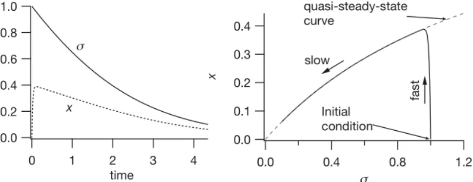
dx/dτis large everywhere, except whereσ−x(σ+κ)is small, of approximately the same size asǫ. Now, note thatσ−x(σ+κ)=0 defines a curve in theσ,xphase plane, called theslow manifold(as illustrated in the right panel of Fig. 1.14). If the solution starts away from the slow manifold,dx/dτ is initially large, and the solution moves rapidly to the vicinity of the slow manifold. The solution then moves along the slow manifold in the direction defined by the equation forσ; in this case,σ is decreasing, and so the solution moves to the left along the slow manifold.
Another way of looking at this model is to notice that the reaction ofxis an ex-ponential process with time constant at least as large as κ
ǫ. To see this we write (1.38) as
ǫdx
dτ +κx=σ (1−x). (1.40)
Thus, the variablex“tracks” the steady state with a short delay. It follows from the quasi-steady-state approximation that
x= σ
σ+κ, (1.41)
dσ dτ = −
qσ
whereq=κ−α= kk2
1s0. Equation (1.42) describes the rate of uptake of the substrate and is called aMichaelis–Menten law. In terms of the original variables, this law is
V= dp dt = −
ds dt =
k2e0s s+Km =
Vmaxs
s+Km, (1.43)
whereKm =k−1k+1k2. In quasi-steady state, the concentration of the complex satisfies
c= e0s s+Km
. (1.44)
Note the similarity between (1.32) and (1.43), the only difference being that the equi-librium approximation usesK1, while the quasi-steady-state approximation usesKm. Despite this similarity of form, it is important to keep in mind that the two results are based on different approximations. The equilibrium approximation assumes that k−1 ≫ k2 whereas the quasi-steady-state approximation assumes that ǫ ≪ 1. No-tice, that if k−1 ≫ k2, then Km ≈ K1, so that the two approximations give similar results.
As with the law of mass action, the Michaelis–Menten law (1.43) is not universally applicable but is a useful approximation. It may be applicable even ifǫ=e0/s0is not small (see, for example, Exercise 14), and in model building it is often invoked without regard to the underlying assumptions.
While the individual rate constants are difficult to measure experimentally, the ratio Km is relatively easy to measure because of the simple observation that (1.43) can be written in the form
1 V =
1 Vmax +
Km Vmax
1
s. (1.45)
In other words, 1/Vis a linear function of 1/s. Plots of this double reciprocal curve are calledLineweaver–Burk plots, and from such (experimentally determined) plots,Vmax andKmcan be estimated.
Although a Lineweaver–Burk plot makes it easy to determineVmax andKm from reaction rate measurements, it is not a simple matter to determine the reaction rate as a function of substrate concentration during the course of a single experiment. Substrate concentrations usually cannot be measured with sufficient accuracy or time resolution to permit the calculation of a reliable derivative. In practice, since it is more easily measured, the initial reaction rate is determined for a range of different initial substrate concentrations.
An alternative method to determineKmandVmaxfrom experimental data is the di-rect linear plot (Eisenthal and Cornish-Bowden, 1974; Cornish-Bowden and Eisenthal, 1974). First we write (1.43) in the form
Vmax=V+V
and then treatVmaxandKmas variables for each experimental measurement ofVands. (Recall that typically only the initial substrate concentration and initial velocity are used.) Then a plot of the straight line ofVmaxagainstKmcan be made. Repeating this for a number of different initial substrate concentrations and velocities gives a family of straight lines, which, in an ideal world free from experimental error, intersect at the single pointVmaxandKmfor that reaction. In reality, experimental error precludes an exact intersection, butVmaxandKmcan be estimated from the median of the pairwise intersections.
1.4.3
Enzyme Inhibition
An enzyme inhibitor is a substance that inhibits the catalytic action of the enzyme. Enzyme inhibition is a common feature of enzyme reactions, and is an important means by which the activity of enzymes is controlled. Inhibitors come in many different types. For example,irreversible inhibitors, orcatalytic poisons, decrease the activity of the enzyme to zero. This is the method of action of cyanide and many nerve gases. For this discussion, we restrict our attention to competitive inhibitors andallosteric inhibitors.
To understand the distinction between competitive and allosteric inhibition, it is useful to keep in mind that an enzyme molecule is usually a large protein, considerably larger than the substrate molecule whose reaction is catalyzed. Embedded in the large enzyme protein are one or moreactive sites, to which the substrate can bind to form the complex. In general, an enzyme catalyzes a single reaction of substrates with similar structures. This is believed to be a steric property of the enzyme that results from the three-dimensional shape of the enzyme allowing it to fit in a “lock-and-key” fashion with a corresponding substrate molecule.
If another molecule has a shape similar enough to that of the substrate molecule, it may also bind to the active site, preventing the binding of a substrate molecule, thus inhibiting the reaction. Because the inhibitor competes with the substrate molecule for the active site, it is called a competitive inhibitor.
Competitive Inhibition
In the simplest example of a competitive inhibitor, the reaction is stopped when the inhibitor is bound to the active site of the enzyme. Thus,
S+E k1
−→ ←−
k−1
C1−→k2 E+P,
E+I k3
−→ ←−
k−3 C2.
Using the law of mass action we find
ds
dt = −k1se+k−1c1, (1.47)
di
dt = −k3ie+k−3c2, (1.48)
dc1
dt =k1se−(k−1+k2)c1, (1.49) dc2
dt =k3ie−k−3c2. (1.50)
wheres= [S],c1 = [C1], andc2= [C2]. We know thate+c1+c2=e0, so an equation for the dynamics ofeis superfluous. As before, it is not necessary to write an equation for the accumulation of the product. To be systematic, the next step is to introduce dimensionless variables, and identify those reactions that are rapid and equilibrate rapidly to their quasi-steady states. However, from our previous experience (or from a calculation on a piece of scratch paper), we know, assuming the enzyme-to-substrate ratios are small, that the fast equations are those forc1andc2. Hence, the quasi-steady states are found by (formally) settingdc1/dt =dc2/dt = 0 and solving forc1 andc2. Recall that this does not mean that c1 and c2 are unchanging, rather that they are changing in quasi-steady-state fashion, keeping the right-hand sides of these equations nearly zero. This gives
c1= Kie0s Kmi+Kis+KmKi
, (1.51)
c2= Kme0i
Kmi+Kis+KmKi, (1.52)
whereKm =k−1k+1k2,Ki=k−3/k3. Thus, the velocity of the reaction is
V =k2c1= k2e0sKi
Kmi+Kis+KmKi =
Vmaxs s+Km(1+i/Ki)
. (1.53)
E
ES
EI
EIS
E + P
k
1s
k
-
1k
1s
k
-
1k
3i
k
-
3k
3i
k
-
3k
2Figure 1.2 Diagram of the possible states of an enzyme with one allosteric and one catalytic binding site.
Allosteric Inhibitors
If the inhibitor can bind at an allosteric site, we have the possibility that the enzyme could bind both the inhibitor and the substrate simultaneously. In this case, there are four possible binding states for the enzyme, and transitions between them, as demonstrated graphically in Fig. 1.2.
The simplest analysis of this reaction scheme is the equilibrium analysis. (The more complicated quasi-steady-state analysis is left for Exercise 6.) We defineKs=k−1/k1, Ki=k−3/k3, and letx,y, andzdenote, respectively, the concentrations of ES, EI and EIS. Then, it follows from the law of mass action that at equilibrium (take each of the 4 transitions to be at equilibrium),
(e0−x−y−z)s−Ksx=0, (1.54)
(e0−x−y−z)i−Kiy=0, (1.55)
ys−Ksz=0, (1.56)
xi−Kiz=0, (1.57)
where e0 = e+x+y+zis the total amount of enzyme. Notice that this is a linear system of equations forx,y, andz. Although there are four equations, one is a linear combination of the other three (the system is of rank three), so that we can determine x,y, andzas functions ofiands, finding
x= e0Ki Ki+i
s Ks+s
. (1.58)
It follows that the reaction rate,V=k2x, is given by
V =1Vmax +i/Ki
s
Ks+s, (1.59)
(The situation is more complicated if the quasi-steady-state approximation is used, and no such simple conclusion follows.)
1.4.4
Cooperativity
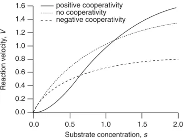
For many enzymes, the reaction velocity is not a simple hyperbolic curve, as predicted by the Michaelis–Menten model, but often has a sigmoidal character. This can re-sult from cooperative effects, in which the enzyme can bind more than one substrate molecule but the binding of one substrate molecule affects the binding of subsequent ones.
Much of the original theoretical work on cooperative behavior was stimulated by the properties of hemoglobin, and this is often the context in which cooperativity is discussed. A detailed discussion of hemoglobin and oxygen binding is given in Chapter 13, while here cooperativity is discussed in more general terms.
Suppose that an enzyme can bind two substrate molecules, so it can exist in one of three states, namely as a free molecule E, as a complex with one occupied binding site, C1, and as a complex with two occupied binding sites, C2. The reaction mechanism is then
S+E k1 −→ ←−
k−1
C1−→k2 E+P, (1.60)
S+C1
k3 −→ ←−
k−3
C2−→k4 C1+P. (1.61)
Using the law of mass action, one can write the rate equations for the 5 concen-trations[S],[E],[C1],[C2], and[P]. However, because the amount of product[P]can be determined by quadrature, and because the total amount of enzyme molecule is con-served, we only need three equations for the three quantities[S],[C1], and[C2]. These are
ds
dt = −k1se+k−1c1−k3sc1+k−3c2, (1.62) dc1
dt =k1se−(k−1+k2)c1−k3sc1+(k4+k−3)c2, (1.63) dc2
dt =k3sc1−(k4+k−3)c2, (1.64)
wheres= [S],c1 = [C1],c2 = [C2], ande+c1+c2=e0.
Proceeding as before, we invoke the quasi-steady-state assumption thatdc1/dt = dc2/dt=0, and solve forc1andc2to get
c1= K2e0s
K1K2+K2s+s2, (1.65)
c2= e0s 2
whereK1 =k−1k+1k2 andK2= k4+k−3
k3 . The reaction velocity is thus given by
V=k2c1+k4c2= (k2K2+k4s)e0s
K1K2+K2s+s2. (1.67) Use of the equilibrium approximation to simplify this reaction scheme gives, as expected, similar results, in which the formula looks the same, but with different definitions ofK1 andK2(Exercise 10).
It is instructive to examine two extreme cases. First, if the binding sites act inde-pendently and identically, thenk1 =2k3=2k+, 2k−1=k−3=2k−and 2k2=k4, where k+andk−are the forward and backward reaction rates for the individual binding sites. The factors of 2 occur because two identical binding sites are involved in the reaction, doubling the amount of the reactant. In this case,
V= 2k2e0(K+s)s K2+2Ks+s2 =2
k2e0s
K+s, (1.68)
where K = k−+k2
k+ is the Km of the individual binding site. As expected, the rate of reaction is exactly twice that for the individual binding site.
In the opposite extreme, suppose that the binding of the first substrate molecule is slow, but that with one site bound, binding of the second is fast (this is large positive cooperativity). This can be modeled by lettingk3→ ∞andk1→0, while keepingk1k3 constant, in which caseK2 →0 andK1→ ∞whileK1K2is constant. In this limit, the velocity of the reaction is
V= k4e0s 2
Km2 +s2 =
Vmaxs2
Km2 +s2, (1.69)
whereKm2 =K1K2, andVmax=k4e0.
In general, ifnsubstrate molecules can bind to the enzyme, there arenequilibrium constants, K1 throughKn. In the limit as Kn → 0 andK1 → ∞while keeping K1Kn fixed, the rate of reaction is
V = Vmaxs n Kn
m+sn
, (1.70)
where Kn
m = ni=1Ki. This rate equation is known as theHill equation. Typically, the Hill equation is used for reactions whose detailed intermediate steps are not known but for which cooperative behavior is suspected. The exponentnand the parameters VmaxandKmare usually determined from experimental data. Observe that
nlns=nlnKm+ln
V
Vmax−V
, (1.71)
so that a plot of ln(V V
max−V)against lns(called aHill plot) should be a straight line of slopen. Although the exponentnsuggests ann-step process (withnbinding sites), in practice it is not unusual for the best fit fornto be noninteger.