Option-implied information and return prediction
JOÃO PEREIRA DE ALMEIDA 152212004
ABSTRACT
Professor José Faias Supervisor
September 15, 2014
Dissertation submitted in partial fulfillment of requirements for the degree of Master of Science in Economics, at Universidade Católica Portuguesa, September 2014.
We prove the existence of a negative variance risk premium for major US stock indexes and stocks, except for relatively high market capitalization stocks. A zero net investment strategy based on log variance risk premium yields an annualized Sharpe ratio of 0.38 and an annualized certainty equivalent of 4.68%. We find that both the log variance risk premium and option-implied betas are negatively priced in contemporaneous and future returns, which is counter intuitive for option-implied betas, given the expected risk return relation.
i
Acknowledgements
I thank Professor José Faias for his continued support and patience in advising my dissertation. I thank him as well for the opportunity of tutoring his Empirical Finance course during the last semester, a rewarding experience which I will take for the rest of my life.
At inception, this technical application was beyond my reach. Learning how to efficiently and correctly (to the best of my ability) handle this amount of data and presenting it in an intelligible and interesting manner took the best part of my days for the past seven months. For this reason, I thank the SAS Institute, and particularly Mr. Jos van der Velden, for kindly allowing me to take part in the SAS Student Fellowship Program, through which I was provided with licenses and other learning resources which quickly moved me through the learning curve. Our implementation also depends very much on the support resources of the Wharton Research Data Services (WRDS) and on the questions and answers available on the website StackOverflow.
My relative success had several contributing factors which were crucial for this long-awaited finale. I thank Católica-Lisbon for the conditions and support provided during my studies. I take this opportunity to acknowledge Professor Guilherme Almeida e Brito and Professor Teresa Lloyd-Braga, who frequently and kindly took the time to personally listen to my views as a member of this institution. It is also of the utmost importance that I thank for the opportunity of tutoring two different courses. Moreover, the very rewarding professional experiences I held during my studies were certainly and in part only attainable due to the quality of my formal education. Finally, I would also like to thank the “Fundação para a Ciência e a Tecnologia”.
I thank my colleagues and friends, who were a cornerstone of my academic success. I recall a number of selfless acts of friendship from people whom I did not know before coming to this institution. It is with joy that I remember the relationships of trust that I have established during my studies.
Above all, I thank my family. A continued effort of generations allowed me to be where I am today. To my family and particularly to my grandparents, my parents, and my siblings I dedicate my work, for it was always conducted with the goal of honoring the effort they put into my education.
ii
Table of Contents
I. Introduction ... 1
II. Data ... 4
III. Methodology ... 6
IV. Variance risk premium ... 16
V. Option-implied betas ... 22
VI. Return prediction using option-implied information ... 24
iii
Index of Tables
Table I. Descriptive statistics of time series average historical market beta ... 7
Table II. Descriptive statistics of time series average option-implied beta ... 9
Table III. Average variance risk premium of index and stocks by size and sectors ... 18
Table IV. Percentage of significant Carhart factors on log variance risk premium ... 20
Table V. Average stock return of log variance risk premium sorted portfolios ... 20
Table VI. Average stock return of option and historical market beta sorted portfolios . 22 Table VII. Fama-Macbeth predictive return regressions for all stocks ... 26
Table VIII. Fama-Macbeth predictive return regressions for S&P 500 stocks ... 27
Table IX. Fama-Macbeth explanatory return regressions for all stocks... 28
Table X. Fama-Macbeth explanatory return regressions for S&P 500 stocks ... 29
Index of Figures
Figure 1. Scatter plot of option-implied betas on historical betas ... 10Figure 2. End-of-month VIX and square root MFIV of the S&P 500 ... 12
Figure 3. Average correlation coefficient and average alpha ... 14
Figure 4. Variance Risk Premium for the S&P 500 Index and average stock ... 16
Figure 5. Performance of stock portfolios sorted on log variance risk premium ... 21 Figure 6. Performance of stock portfolios sorted on option-implied and historical beta 23
1
I. Introduction
Option-implied information is relevant for the prediction of future stock returns [Chakravarty, Gulen, and Mayhew (2004), Pan and Poteshman (2006), Goyal and Saretto (2009), Vasquez (2012)]. A particular usage of option-implied information is calculation of the expected variance through the use of out-of-the-money implied volatility. This figure may be used to calculate the variance risk premium, the difference between the realized variance and the expected variance over a period of time. The variance risk premium has been shown to be on average negative for major US stock indexes. [Carr and Wu (2009)]. Research has also shown that the expected variance risk premium is negatively related with future stock returns [Han and Zhou (2011)]. Additionally, this option-implied variance may be used to calculate the betas of a stock relative to an index. These betas have been shown to, on average, respect the expected risk-return relation [Buss and Vilkov (2012b)].
In this work we join these two strands of the option-implied information literature and test the simultaneous predictive and explanatory power of past variance risk premia and forward-looking betas of the monthly returns for all CRSP stocks through the use of Fama-Macbeth regressions between January 1996 until August 2013. We successfully define an investment strategy based on the positive return spread between low and high variance risk premium stocks. Moreover, we find that both the log variance risk premium and the option-implied beta are significant in predicting future monthly stock returns for the stocks in our sample, but not for the S&P 500 constituents’ subsample. Both factors are priced negatively in future returns, which is counterintuitive for option-implied betas. Regarding explanatory regressions, we find that both these factors are significant return factors for the entire sample, including the S&P 500 constituents’ subsample, and that again both are negatively priced.
Ever since Markowitz (1952) that studying the factors priced in security returns has been a thoroughly researched topic. The first relevant model for this is the CAPM, attributed to the simultaneous research of Sharpe (1964), Lintner (1965a) and Lintner (1965b), and Mossin (1966), which relates the expected returns of a stock with its covariance with the market portfolio.1 Studies such as Fama and MacBeth (1973)
1
2 initially confirmed the empirical relevance of the exposure to the market portfolio in stock pricing. Later, Fama and French (1992) tested the significance of additional factors in explaining stock returns, based on the relevance of firm specific characteristics such as size [Banz (1981)], book-to-market [Rosenberg, Reid, and Lanstein (1985)], leverage [Bhandari (1988)] and earnings-price ratio [Basu (1983)]. They concluded with Fama and French (1993) which proposes the commonly used three factor model, using market risk premium, small-minus-big size, and high-minus-low book-to-market portfolio returns, the two latter based on zero net investment strategies. Since then, more factors for stock pricing have been successfully proposed, such as the momentum factor [Jegadeesh and Titman (1993)] or the liquidity factor [Pastor and Stambaugh (2001)]. Additionally, factors have been proposed to the price the exposure of option strategies, namely those of index straddle returns [Coval and Shumway (2001)]. Predicting returns is another strand of literature, for which Rapach and Zhou (2012) provide a good overview. With the use of linear models to predict the equity premium, Goyal and Welch (2008) find little evidence of statistically significant out-of-sample performance of commonly suggested equity premium predictors. More promising results are possible through different model specifications [Rapach and Zhou (2012)]. Our results follow more closely the literature of explanatory regressions, as they are not concerned with the relative performance of the predictive effort, but rather in testing whether our suggested factors are significantly priced in future returns.
Option-implied information provides superior future returns. Chakravarty, Gulen, and Mayhew (2004) show there is significant stock price discovery in the option market and that it may lead stock markets, namely in the case of high volume options and low volume stocks. According to Pan and Poteshman (2006) the relative volume of new put trades (as opposed to positions opened in order to close old positions) is linked to future returns. Goyal and Saretto (2009) show that deviations of the volatility implied exclusively by the at-the-money option prices from the historical volatility can be used to define a successful investment strategy on straddles of the underlying stocks. In a strategy similar to this, Vasquez (2012) show that securities with small difference between the annualized 365-day and 30-day variance expectations (i.e. variance term premium) tend to have significantly negative average straddle returns, while high variance term premium stocks tend to have significantly positive average straddle returns. Recall that straddles are composed by one long at-the-money put option and
3 one long at-the-money call option, profiting from increases in volatility. Consequently, we believe there is sufficient evidence that some option-implied information may be priced in future returns.
We build on this literature to conclude whether option-implied betas and the variance risk premium are significantly priced in stock returns. For this, we first analyze and document the existence of a variance risk premium between the realized and expected variance of a security. For this purpose, we expand the sample of Carr and Wu (2009). Secondly, we analyze whether the past variance risk premium and the forward looking betas of Buss and Vilkov (2012b) can significantly predict future monthly returns when simultaneously regressed with historical Fama-French and Carhart betas. Our hypotheses are that option-implied betas are positively priced in future returns, following the expected risk-return relation, and that variance risk premia are negatively priced in future returns [Han and Zhou (2011)].
The usage of information implied by option prices for investment purposes is increasingly familiar to investors. One of the most recognized implementations of option based information is the CBOE Volatility Index (known as the VIX Index). Frequently referred to as the “fear index” in financial media, the VIX Index reflects the market expectations of 30-day volatility of the S&P 500 Index, through the information on future volatility contained on S&P 500 index option prices.2 Though the underlying asset of these options focuses on the large market capitalization segment, it encompasses 80% of the available U.S. market capitalization, making it a good proxy for the overall U.S. equity markets volatility.3 Investing in the VIX Index could serve a hedging or speculative purpose. It is relevant to state that the time series of log returns of the VIX Index and the S&P 500 show a Pearson correlation coefficient of -0.70 between 1990 and 2014. Through that figure, it becomes evident why increases in volatility are frequently associated with decreasing returns. Though the CBOE offers future contracts on the VIX Index, actually going long on such an index is difficult for
2 A good overview of the VIX and its calculation methodology is offered by the information
available on the CBOE’s product page: http://www.cboe.com/micro/VIX/vixintro.aspx
4 an investor – although there are several Exchange Traded Funds available, references in the financial media to poor tracking are far from uncommon.4
This work is organized as follows. In Section II we present details on the data. In Section III we present the methodology. In Section IV we study the sign of the variance risk premium and its average predictive power. In Section V we compare the average predictive power of historical and option-implied market betas. In Section VI we study the return explanatory and predictive power of the variance risk premium, historical betas, and option-implied market betas. In Section VII we conclude.
II. Data
We use CRSP for stock price data, OptionMetrics for option data, and the Kenneth French data library for asset pricing factors. Specifically, we extract from the latter standard Carhart factors (market risk premium, small minus big, high minus low, and winners minus losers momentum), and the one-month Treasury bill rate of Ibbotson Associates, to use as inputs in the historical beta regressions.5
Our analysis focuses on all CRSP ordinary common shares (share code 10 and 11), excluding non-US companies, trust companies, exchange traded funds, closed-end funds, and REITs which we can uniquely match in OptionMetrics and that are traded between January 1996 and August 2013 [Bali and Hovakimian (2009)]. This leaves us with 23,635 unique CRSP stock identifiers (PERMNO) from a total of 30,068 unique stocks in CRSP. We then match Ivy Db’s OptionMetrics and CRSP. We obtain 13,045 unique PERMNOs to SECID matches.6 These securities form the base sample. Our sample is limited in more ways than this. We can only estimate model-free implied variance for 5,888 unique stocks. Moreover, our predictive analysis is conducted only with observations for which we have a lagged variance risk premium, an estimate for its
4 See, for instance, “VIX ETFs: An imperfect hedge” and “The risks of VIX-tied investing”, the
latter written by the creator of VIX, Professor Robert Whaley, respectively available on: http://finance.yahoo.com/news/vix-etfs-imperfect-hedge-150919196.html and http://www.cnbc.com/id/101738018
5 The Kenneth French data library is publicly available at
http://mba.tuck.dartmouth.edu/pages/faculty/ken.french/data_library.html and is also accessible through WRDS.
6 We accomplish this by using a SAS research macro kindly made available on the Wharton
Research Distribution Services. This reduction from 23,635 to 13,045 stocks is understandable, given that OptionMetrics only has records from January 1996 onwards, while CRSP goes back to 1927 in some instances.
5 option-implied beta, and its historical betas. By requiring these simultaneously, our sample is overall reduced to 3,451 unique stocks.
We resort to CRSP for dividend and stock-split adjusted simple daily returns, which we transform into log returns. We them sum these within each month for each security to obtain monthly returns, requiring at least 15 observations in a month for a valid return (note that, consequently, this excludes September 2001). In order to have Carhart historical betas at the beginning of our sample in January 1996, we use returns from January 1991. We also use the daily adjusted returns to calculate end-of-month realized variance. Exceptionally, we extract the annualized realized variance for stock indexes from the OptionMetrics historical volatility file, since the index prices are not easily extractable from CRSP (an index does not have a PERMNO and is stored on a separate dataset). This does not change our results as we only use index variance risk premia for presentation purposes, not for analytical results.
To obtain the S&P 500 members in each moment of time, we use an S&P 500 constituents file from CRSP, with addition and deletion date by PERMNO. We select all those that are currently members of this index or have been deleted from it after 1st January 1996. From January 1996 until August 2013 there are 984 member stocks, of which 970 unique stocks (a number of stocks exit and reenter the index). By using our matching database, we are able to match 891 of these stocks. Consequently, the average number of matched member stocks throughout our sample period is 461 companies, ranging from a minimum of 449 to a maximum of 468. Our S&P 500 index weights are calibrated so that only the market capitalization of the matched stocks is considered.
After limiting our database to the records which simultaneously have all the variables under analysis, our stocks show an average monthly return of 0.21%, an average historical market beta of 1.19, and an average market capitalization of $7,039 million, whereas the S&P 500 constituents present an average monthly return of 0.70%, an average historical market beta of 1.13 and an average market capitalization of $17,778 million.
We use the end-of-month Volatility Surface of option-implied volatility and strikes provided by OptionMetrics to compute the model-free implied variance, our forecast of 30-day variance. Additionally, we use the Security Information files available on OptionMetrics to divide the sample in sectors and indexes.
6
III. Methodology
To simultaneously test the predictive power of historical asset pricing factors and option-implied information, we use monthly returns adjusted for dividends and stock splits, historical monthly betas, variance risk premia and forward looking option-implied market betas for every security, at the end of each month. In this subsection we go into further detail on how we estimated each of these elements. Unless otherwise stated, all hypothesis testing is conducted with a 5% significance level.
A.1. Historical Betas
On each month t we estimate a Carhart asset pricing model through Ordinary Least Squares (OLS) for each security i, using data from month t-60 up to month t:
(1)
where MRP is the Market Risk Premium (based on the application of Sharpe (1964)), HML is the High-Minus-Low book-to-market zero net investment portfolio [Fama and French (1993)], SMB is the Small-Minus-Big market capitalization zero net investment portfolio [Fama and French (1993)], and MOM is the Winners-Minus-Losers Momentum zero net investment portfolio [Jegadeesh and Titman (1993), Carhart (1997)]. These are the most commonly used equity asset pricing factors.
In Table I we show the descriptive statistics of the average historical market beta, estimated through a Carhart model, by sector and size quintile. We only present this coefficient as it is comparable to our option-implied market beta. When comparing an average stock with an average S&P 500 stock, we see that the former has, on average, a lower market beta. We also find a negative relation between size and average beta, along with some industry fluctuation in average betas, where Construction and Transportation, Communication, Electricticity and Gas show the highest average values, while Mining, Wholesale & Retail Trade show the lowest average values.
7
Table I. Descriptive statistics of time series average historical market beta
In this table we present descriptive statistics of the average historical market beta based on a Carhart model. We first split the securities at the end of each month whether they are, were, or will be an S&P 500 constituent (average stock panel) and according to their end-of-month market capitalization (size panel), and SIC code (industry panel). Then we average the historical betas at the end of the month, obtaining a time series for each subsample. The values presented are on that time series. This may be interpreted as the beta for the average stock in any of these subsamples at any moment of our sample period. Mean, Standard Deviation are the standard descriptive statistics, P10 and P90 identify the 10% bottom and upper (respectively) cutoff points in the sample.
Time Series Average Beta
Mean Std. Dev. P10 P90 Min Max
Average Stock 1.19 0.04 1.13 1.23 1.09 1.27
Average S&P 500 Stock 1.13 0.05 1.07 1.21 1.03 1.25
Stocks by Size Q1 – Small 1.35 0.09 1.24 1.49 1.18 1.58 Q2 1.23 0.06 1.16 1.32 1.11 1.38 Q3 1.17 0.07 1.09 1.27 1.05 1.39 Q4 1.14 0.07 1.05 1.23 1.00 1.30 Q5 – Big 1.05 0.06 0.97 1.13 0.91 1.17 Stocks by Industry
0 – Agric., Forestry, And Fishing 1.09 0.44 0.36 1.57 0.00 2.02
1 - Mining 0.84 0.28 0.58 1.22 0.16 1.43
2 - Construction 1.40 0.20 1.14 1.64 0.93 1.95
3 - Manufacturing 1.03 0.10 0.86 1.13 0.82 1.18
4 - Transp., Comm, Electric, Gas etc. 1.33 0.13 1.12 1.50 1.05 1.58
5 - Wholesale & Retail Trade 1.01 0.07 0.94 1.11 0.88 1.15
6 - Fin., Insurance, And R. Estate 1.06 0.09 0.97 1.19 0.84 1.30
7 - Services 1.17 0.19 0.95 1.47 0.84 1.53
8 - Services 1.27 0.11 1.11 1.45 1.04 1.54
9 - Public Administration 1.15 0.20 0.92 1.44 0.83 1.72
No information 1.14 0.06 1.07 1.19 1.05 1.46 A.2. Option Implied Betas
Buss and Vilkov (2012b) estimate option implied betas by resorting to the risk-neutral measures of expected variance and correlation. Their option-implied beta is, simply put, the covariance of a security with all the remaining securities in the market index (which we assume as the S&P 500) divided by the market variance, replacing the usual historical moments for their risk-neutral counterparts. This expression is equivalent to the coefficient obtained from an OLS regression of a single variable asset pricing model. The option-implied market beta of a security i at time t is defined as:
8 where N is the total number of securities in the market portfolio for which we can successfully estimate variance and risk-neutral correlation, w stands for the market capitalization weight of security j. MKT stands for the market. Throughout the following sections, the superscript P denotes the realized measure, while Q denotes the risk-neutral measure. Since we do not define option-implied betas for any other pricing factor, we will refer to this market beta simply as option-implied beta.
Two cautionary notes are necessary. First, given that we use the S&P 500 as our market index, N should not significantly differ from 500 at any time. However, it does. Our constituents fluctuate between 449 and 468. This has three fundamental reasons. First, matching all members of the index between CRSP and OptionMetrics is not straight-forward, as is discussed Section II. Secondly, we may exclude a security from the option-implied variance calculation if our volatility extrapolation-interpolation routine fails. Thirdly, a member stock may not yet have a 60-month correlation with the other stocks in the portfolio, making it ineligible for inclusion. Besides this discrepancy in defining the member stocks, another cautionary note is need. Note that factor models are usually expressed in terms of risk premium for the stock and the market factor. Our specification does not encompass this possibility, since there are no options traded on the risk premium of a stock. Surpassing this limitation is a suggestion for further research.
In Table II we show descriptive statistics of the average option-implied beta. We find the same patterns regarding the average stocks in our sample, where the S&P 500 stocks have lower average betas. Again we detect the same negative relation between size and beta. However, by contrast with Table I, we can see that the average option implied market beta across time is higher than its historical counterpart and also that it has greater variability. The same descending pattern can be seen in size quintiles and higher average betas are also observed on the full sample of stocks than in the S&P 500 constituents’ subsample.
9
Table II. Descriptive statistics of time series average option-implied beta
In this table we present descriptive statistics of the average option-implied beta. Grouping of observations and statistics are defined as those of Table I.
Time Series Average Option-Implied Beta
Mean Std. Dev. P10 P90 Min Max
Average Stock 1.45 0.22 1.16 1.69 0.77 2.06
Average S&P 500 Stock 1.19 0.11 1.04 1.31 0.84 1.41
Stocks by Size Q1 – Small 2.00 0.42 1.44 2.50 0.67 3.23 Q2 1.57 0.28 1.18 1.88 0.68 2.34 Q3 1.37 0.21 1.09 1.60 0.77 1.93 Q4 1.23 0.16 1.03 1.42 0.76 1.67 Q5 - Big 1.08 0.06 1.00 1.15 0.89 1.21 Stocks by Industry
0 – Agric., Forestry, And Fishing 1.05 0.29 0.65 1.44 0.32 1.95
1 - Mining 1.48 0.35 1.06 1.94 0.71 2.46
2 - Construction 1.40 0.26 1.07 1.71 0.66 2.02
3 - Manufacturing 1.58 0.23 1.30 1.87 0.87 2.15
4 - Transp., Comm, Electric, Gas etc. 1.21 0.20 0.90 1.43 0.58 1.68
5 - Wholesale & Retail Trade 1.36 0.21 1.06 1.60 0.71 1.97
6 - Fin., Insurance, And R. Estate 1.32 0.28 1.04 1.73 0.86 2.02
7 - Services 1.60 0.24 1.29 1.89 0.76 2.22
8 - Services 1.47 0.32 1.12 1.90 0.56 2.18
9 - Public Administration 1.46 0.46 0.90 2.08 0.45 3.00
No information 1.21 0.27 0.76 1.50 0.52 1.55
When regressing the option-implied market beta on the historical market beta, by month, we obtain an average intercept of 0.89 and a slope coefficient of 0.46. All observations of the intercept and slope coefficients are positive, which suggests that there is a positive relation between option-implied beta and historical beta, and that there is an average positive bias on the option-implied beta. Figure 1 exemplifies this for January 2006, where the red marks identify an S&P 500 constituent and the blue marks identify a non S&P 500 constituent. In this sampling, we observe much greater variability in the non-S&P 500 stocks, creating larger differences between the option-implied and historical betas.
10
Figure 1. Scatter plot of option-implied betas on historical betas
This figure compares the historical market beta and the option-implied market beta for each stock in our sample for January 2006. Each mark represents a stock. Blue marks identify a non-S&P 500 constituent and red marks identify an S&P 500 constituent. The horizontal axis displays the historical market beta calculated for the past 60 consecutive months, while the vertical axis displays the option-implied market beta at the end of January 2006. We limit the sample to a single month due to the computational effort required for larger scatter plot. Linear regression of historical market beta on a constant and option-implied market beta fit with OLS.
We now explain how to obtain the several inputs for the option-implied betas. Risk-neutral variance expectations of stocks may be inferred from option data (Part A.3). Since there are no assets traded on the correlation between every pair of stocks, we infer the risk-neutral correlation based on historical rolling five year (i.e. 60 past monthly observations) correlation and a modeling choice of Buss and Vilkov (2012b) (part 0), considering the existence of a correlation risk premium, as proven by the correlation factor in Driessen, Maenhout, and Vilkov (2009).
A.3. Model-Free Implied Variance
Based on the Volatility Surface provided by OptionMetrics, it is possible to observe several pairs of implied volatility and strike for a given security, for a range of standardized maturities (30, 60, 91, 182, 365, 547, and 730 days). We focus on the 30-day maturity and filter only those options which have delta (an option’s sensitivity to change in the underlying asset’s spot price) lower than 0.5 in absolute value, in order to
11 get the out-of-the-money options. This choice for out-of-the-money options is related to their greater liquidity. From Bakshi, Kapadia, and Madan (2003), the model-free implied variance (MFIV) between time t and time is:
(3)
In essence, this formula combines out-of-the-money puts and calls for a continuum of strikes. Since we do not have a continuum of strikes in the market, the formula needs to be approximated. According to the discretization scheme used, this involves first interpolating and extrapolating the implied volatility across a moneyness grid between 1/3 and 3 with 1,001 points. For a moneyness point inside the range of sample moneyness, we interpolate the variance using cubic splines, with a spline knot on each sample observation. For a moneyness point outside the range of sample moneyness, we extrapolate that the implied volatility is the same as that of the minimum or maximum interpolated points. In case our extrapolation-interpolation procedure results in negative implied-volatility for any moneyness, we exclude that security on that specific day from the analysis. We then price out-of-the money calls or puts (depending on the moneyness) through the Black-Scholes pricing model [Black and Scholes (1973)] for each of the interpolated-extrapolated implied volatility-moneyness pairs and apply the integral discretization scheme to obtain the model-free implied volatility of Bakshi, Kapadia, and Madan (2003). For the Black-Scholes pricing, we use the 30-day zero coupon rate available on OptionMetrics as an input. The expectation for variance we obtain is monthly, which we then annualize under the 365/30 convention. For simplification of the notation, instead of presenting the expectation operator of the annualized future realized variance and since we always use a 30-day maturity, we refer to the MFIV of an asset i at the end of month t-1 as or .7
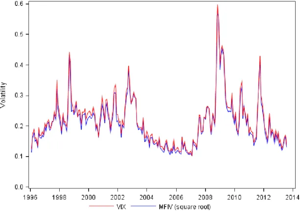
To benchmark the quality of our measure of volatility, at the end of each month we compare the square root of the 30-day MFIV of the S&P 500 with the VIX Index, from January 1996 until September 2013. Our methodology is different from that of the VIX Index. Nevertheless, these two series should be quite similar, as they aim to
7 We adapt to SAS the MATLAB discretization used by Buss and Vilkov (2012a), kindly provided
on Grigory Vilkov’s website, which follows the methodology of Bakshi, Kapadia, and Madan (2003) for model-free implied moments.
12 forecast the same variable, for the same time period. On average, our measure is lower than that of the VIX by 0.01 in terms of volatility (this average difference is statistically significant at a 1% level, suggesting that there is a systematic difference in the calculation methodology). Nevertheless, we can see by Figure 2 that the two series consistently track each other – in fact, the pair presents a Pearson correlation coefficient of .997.
Figure 2. End-of-month VIX and square root MFIV of the S&P 500
This figure presents the end-of-month VIX Index and the square root of our calculated model-free implied variance. The red line is the VIX Index, while the blue line is the square root of the Model-Free Implied Variance described in Part A.3 based on the volatility surface of S&P 500 index options.
The VIX Index, however, is not enough for our purpose, as we aim to estimate the MFIV for all each in our sample. The MFIV of each stock is not tracked in the market, unlike how the S&P 500 30-day volatility expectations are by the VIX Index.
A.4. Risk-neutral measure of correlation
Correlation, as variance, is not an observable parameter in the market. Additionally, there are no traded options that allow us to infer the covariance of two securities. That being the case, we need to estimate the risk-neutral measure of correlation. For this purpose and for consistency in the application of the option-implied
13 betas, we also follow the methodology of Buss and Vilkov (2012b) for the estimation of the risk-neutral measure of correlation.
As shown in Equation (4), it is assumed that the risk-neutral expectation of market variance is the summation of the risk-neutral measure of covariance between all the N assets in the market portfolio (in our case, the S&P 500).
(4) In this equation, all we cannot conclude based on market and option information is the risk-neutral measure of correlation. Considering the existence of a correlation risk premium, as evidenced by Driessen, Maenhout, and Vilkov (2009), Buss and Vilkov (2012b) adopt the modelling choice of Equation (5) for the risk-neutral measure of correlation based on the true measure of correlation:
(5)
According to Buss and Vilkov (2012b), this modelling choice stands on two assumptions, based on empirical observation. First, that the risk-neutral measure is usually higher than the true measure. Secondly, that this premium between the risk-neutral measure and the true measure is greater for stocks with low or negative correlation. Consequently, this modelling choice satisfies the first condition if the parameter and the second one if . However, the only necessary condition for the risk-neutral measure to be bounded in absolute value to a maximum of one is that . That being said, we then need to estimate the parameter at the end of each month. For this, we take the restriction of Equation (4) and substitute the risk-neutral measure by its expression in (5) and solve for alpha. This results in Equation (6), which we solve on a monthly basis.
(6)
As a proxy for the true measure, we use the historical correlation coefficient of the past 60 months, the same lag used in historical beta estimation. After calculating , we then have all necessary inputs to calculate the option-implied beta of each security, each
14 month. Note that we only need correlations between all securities and index member stocks, not between all stocks, which greatly reduces the computational effort.
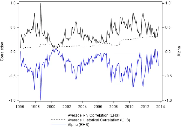
Figure 3. Average correlation coefficient and average alpha
This figure presents both time series of average risk neutral and historical correlation coefficients between all stocks in the sample and S&P 500 members. Additionally, the time series of the calibrated alpha is shown. The filled black line shows the average risk-neutral correlation, the dotted black line shows the average historical correlation coefficient and the filled blue line shows the average alpha. Average correlation coefficients are computed as the end of month cross sectional average across all computed correlations. Each correlation coefficient is calculated based on 60 month past returns.
In Figure 3 we present the evolution of , the average end-of-month risk-neutral and historical correlation coefficients across all stock-member stock pairs. The high variability of is noticeable, which consequently makes the average risk-neutral correlation coefficient vary substantially. In our estimation, the absolute value of is not always negative, which reverses the correlation risk premium on 12 months. Additionally and more importantly, our calibration produces an alpha larger than one in absolute value for August 1998 (-1.03). We truncate this value to -1 to guarantee that all correlations are lower than one. In fact, this observation makes all assets become perfectly correlated (see Equation (5) and substitute alpha with -1). This is not an expected result, nor do we believe it would hold had we all information for all member stocks of our benchmark index, at all moments. Moreover, we believe that alpha calibration may be better suited for usage with daily correlations, rather than monthly.
15 In Buss and Vilkov (2012b) it is stated that, according to their results, . However, no statistics or plots on alpha are provided so that we can benchmark our time-series.
A.5. Variance Risk Premia
We define the Variance Risk Premium as the difference between the annualized realized variance of a certain security over month t and the annualized risk-neutral expectation of variance of that same security at the end of month t-1:
(7)
which, to normalize the series, we also analyze as a natural logarithm:
(8)
Following the 365/30 convention, the annualized realized variance is given by:
(9)
where T(t) is the number of trading days in month t.
There are alternative ways to compute the realized variance. For instance, Carr and Wu (2009) calculate the Realized Variance with future prices. However, we adopt this formulation because it appears to be the standard used in the variance futures on the S&P 500 Index traded on the CBOE and also because of its ease of technical implementation.8
In Figure 4 we present the variance risk premium of the S&P 500 Index and the cross-sectional average variance risk premium for all OptionMetrics stocks at the end of each month. It can be seen that this figure is on average slightly negative, more so for the stocks than for the index. Additionally, the decile bands allow us to see that, while there is some cross sectional fluctuation, this figure appears to be correlated across deciles.
8
These futures are called “VA”. For more details, see S&P 500 Variance Future contract specifications: http://cfe.cboe.com/Products/Spec_VA.aspx
16
Figure 4. Variance Risk Premium for the S&P 500 Index and average stock
This figure presents a time series of the variance risk premium of both the S&P 500 (Panel A) and of the average variance risk premium of all sample stocks (Panel B). Note that the scale in each panel is different. The vertical axis is in the units of the VRP, in squared percentage points. The gray bands in Panel B mark the limits of the vertical axis of Panel A.
IV. Variance risk premium
Our initial objective is to calculate the Variance Risk Premium for all stocks in our sample, largely expanding Carr and Wu (2009). We test the existence of significantly non-zero variance risk premium for stock indexes and individual stocks. Additionally, we test the explanatory power of the Carhart factors for the individual stock’s variance risk premium. Finally, we develop an investment strategy based on athe magnitude of the variance risk premium of the stocks.
A. Significance and explanatory analysis
As shown, market expectation of future variance may be implied through option pricing data. When compared against the verified realized variance in the market, either for an index or specific security, Carr and Wu (2009) show that the difference between the realized variance and the expected variance over periods of one month is significantly negative for U.S. equity indexes, for the period between 1996 until 2003. Additionally, they obtain mixed results for their selection of 35 individual stocks, with
17 only 7 showing a significantly negative average. This significant negative average difference is explained economically by Carr and Wu (2009) as insurance against volatility surges, typically associated with negative returns. This is better understood through an investment in variance, such as the futures on the variance of the S&P 500 traded on the CBOE or Variance Swaps on individual stocks through OTC transactions (in these contracts, the strike variance is referred to as the variance swap rate).9 The payoff of these instruments (neglecting minor adjustments for margin accounts and their accrued interest) is the difference of Equation (7), multiplied by a notional amount. In that sense, and since these are contracts with zero initial investment, the strike, measured in variance, should be equal to the risk neutral expectation of variance over the contract period. In that case, and by proving the existence of a significantly negative average variance risk premium for stocks and indexes, we can state that investors going long on these contracts (i.e. paying the floating leg, the realized variance) should on average lose – and since the payoff is a zero-sum game, the short leg of the contract should on average earn a positive payoff.
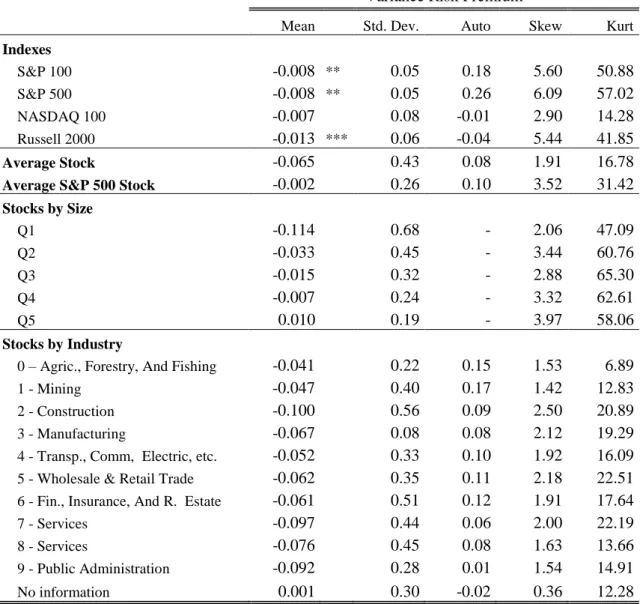
We first subdivide the sample between stocks and indexes, sub-periods, and sectors, which we present in Table III. We conclude that the variance risk premium is statistically significant for the major U.S. equity indexes, namely for large market capitalization indexes such as the S&P 100 Index and the S&P 500 Index, or for small market capitalization indexes, as the Russell 2000 Index. These findings are consistent with Carr and Wu (2009), though our average values are less negative. This may be explained by the differences in the sample time-span, and the fact that our sample includes the 2008 financial crisis, in which variance peaked. We are unable to conclude the same for the NASDAQ 100 Index. Also, the average values and their standard deviation appear to be more negative for indexes with more small capitalization stocks, such as the Russell 2000 Index. The average stock in our sample presents a substantially more negative average variance risk premium if it is not an S&P 500 stock, although also presenting greater variability. The same pattern may be observed when comparing the average stock in our sample with the average constituent stock of the S&P 500. In of Table III we observe a decreasing pattern in the Variance Risk Premium as size grows – in fact, in the largest quintile of stocks, we see a positive average Variance Risk
9 Demeterfi et al. (1999) provide a very good understanding of the structure and pricing of such
18 Premium. Regarding the industry analysis, we find negative average values across the stocks in each industry and along our sample period, except for those without SIC code.
Table III. Average variance risk premium of index and stocks by size and sectors
This table presents descriptive statistics on the average variance risk premium of the stocks in our sample. The descriptive statistics for the index panel are calculated based on their time series. Bilateral tests on the average being equal to zero are conducted on the first panel for indexes. *, **, and *** denote a 10%, 5%, and 1% or lower p-value of the test statistics, respectively. All standard errors are corrected according to Newey and West (1987) with 1 lag autocorrelation. Those of the average stock panel are calculated as the cross sectional average of the time series descriptive statistics for all stocks. The same is applicable for the SIC code panel, except the cross section of stocks is divided according to their industry. The descriptive statistics of the size panel are calculated for a time series of cross sectional average variance risk premia of stocks in each size quintile at each moment of time. This was adopted because stocks jump between quintiles in time and, therefore, allocating a stock to one quintile could imply that its statistics had the same weight if it only was classified in that quintile for a day or for a year. For this reason, no average autocorrelation coefficient is presented. In the same manner, note that the kurtosis cannot be interpreted as the average kurtosis of a stock of each decile but rather the kurtosis of the time series of the average variance risk premium.
Variance Risk Premium
Mean Std. Dev. Auto Skew Kurt
Indexes S&P 100 -0.008 ** 0.05 0.18 5.60 50.88 S&P 500 -0.008 ** 0.05 0.26 6.09 57.02 NASDAQ 100 -0.007 0.08 -0.01 2.90 14.28 Russell 2000 -0.013 *** 0.06 -0.04 5.44 41.85 Average Stock -0.065 0.43 0.08 1.91 16.78
Average S&P 500 Stock -0.002 0.26 0.10 3.52 31.42
Stocks by Size Q1 -0.114 0.68 - 2.06 47.09 Q2 -0.033 0.45 - 3.44 60.76 Q3 -0.015 0.32 - 2.88 65.30 Q4 -0.007 0.24 - 3.32 62.61 Q5 0.010 0.19 - 3.97 58.06 Stocks by Industry
0 – Agric., Forestry, And Fishing -0.041 0.22 0.15 1.53 6.89
1 - Mining -0.047 0.40 0.17 1.42 12.83
2 - Construction -0.100 0.56 0.09 2.50 20.89
3 - Manufacturing -0.067 0.08 0.08 2.12 19.29
4 - Transp., Comm, Electric, etc. -0.052 0.33 0.10 1.92 16.09
5 - Wholesale & Retail Trade -0.062 0.35 0.11 2.18 22.51
6 - Fin., Insurance, And R. Estate -0.061 0.51 0.12 1.91 17.64
7 - Services -0.097 0.44 0.06 2.00 22.19
8 - Services -0.076 0.45 0.08 1.63 13.66
9 - Public Administration -0.092 0.28 0.01 1.54 14.91
19 To test the sign of each asset’s variance risk premium, we limit the sample to those stocks with more than 20 variance risk premium observations. Out of the resulting 3,451 firms, 2,470 (1,118) show a (significant) negative average variance risk premium and 981 (24) show a (significant) positive average variance risk premium. By conducting the same exercise for S&P 500 constituents, out of 804 firms with more than 20 variance risk premium observations, 478 (167) show a (significant) negative average variance risk premium and 328 (9) show a positive (significant) average variance risk premium. We confirm the negative variance risk premium hypothesis for fewer stocks (in relative terms) when considering only S&P 500 constituents. In that sense, we again observe the relevance of size in the sign of the variance risk premium.
Regarding autocorrelation, we observe low average values. We relate this to the finding of Carr and Wu (2009) who describe that the autoregressive process of the variance is not passed on to the variance risk premium. In fact, both the realized variance and the model free implied variance of these series (not shown) show substantially higher average autocorrelation values.
Finally, in Table III we see moderate values for skewness and high values of kurtosis in the variance risk premium, which motivated Carr and Wu (2009) to use the log of the ratio between realized variance and the swap rate. We follow the same reasoning and henceforth use the log variance risk premium.
In the same line of Carr and Wu (2009), we test whether the individual Variance Risk Premium is explained by the Carhart factors, by running the following regression for each security during our sample period:
(10)
where MRP is the Market Risk Premium, HML is the High-Minus-Low book-to-market zero net investment portfolio, SMB is the Small-Minus-Big market capitalization zero net investment portfolio, and MOM is the Momentum zero net investment portfolio.
In line with Carr and Wu (2009), we see high cross sectional variability in terms of explanatory power, with R2 ranging from 0.1% to 77% (0.2% to 70%) for all stocks (for S&P 500 constituents) However, such high R2 values are limited in the sample. The median R2 is 10.1% (6.5%). The bottom and upper 10% percentile are 2% (2.9%) and
20 30% (18.4%), respectively. We see lower global significance in the cross section of S&P 500 constituents. This is confirmed by an individual analysis, as presented in Table IV where a much larger percentage of the individual coefficients in Equation (10) reject the null hypothesis of being equal to zero in the overall sample than in the S&P 500 constituent subsample. Overall, we see low global and individual significance and we only do not reject the significance of the factors for a reduced part of our sample.
Table IV. Percentage of significant Carhart factors on log variance risk premium
This table presents the percentage of assets for which the null hypothesis of a given Carhart coefficient being equal to zero is rejected in a model of monthly variance risk premia. The null hypothesis is that each individual coefficient on Equation (10) is equal to zero. The equation was estimated for the period between February 1996 and August 2013. Hypothesis testing conducted with 5% significance level. Standard errors corrected according to Newey and West (1987) for 1 lag autocorrelation. N stands for the number of stocks in each subsample.
% of null rejection N
All stocks 3,451 31.56 19.53 20.14 22.08 23.09
S&P 500 constituents 808 8.14 3.77 4.55 5.51 5.16
B. Future returns of variance risk premium portfolios
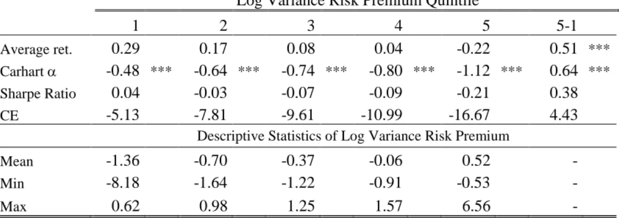
Table V. Average stock return of log variance risk premium sorted portfolios
This table presents portfolio performance measures for quintile portfolios based on the log variance risk premium of the stocks in our sample. Quintile portfolios are formed at the end of each month t-1, based on the log variance risk premium in month t-1. All returns are presented in percentage points. Returns are the equally weighted average monthly return of the stocks in each quintile portfolio for month t. The Carhart is the constant in a Carhart model, as that of Equation (1), of each portfolio’s excess return relative to the one month Treasury bill rate. The Sharpe Ratio is the annualized ratio between the average monthly excess return of each portfolio relative to the one month Treasury bill rate divided by the standard deviation. To annualize it we multiply the calculated Sharpe Ratio by square root of 12. CE stands for Annualized Certainty Equivalent. It is calculated with a power utility function with a risk aversion coefficient of 4 and annualized by multiplying the resulting certainty equivalent by 12. Mean, max, and min are the time series averages of the average, maximum, and minimum log variance risk premium at each moment of time in each quintile, respectively. Significance analysis is conducted for both the average return and the Carhart with Newey-West standard errors with 1 lag autocorrelation. The null hypothesis tested is that the average is equal to zero. *, **, and *** denote a 10%, 5%, and 1% or lower p-value of the test statistics, respectively.
Log Variance Risk Premium Quintile
1 2 3 4 5 5-1
Average ret. 0.29 0.17 0.08 0.04 -0.22 0.51 *** Carhart -0.48 *** -0.64 *** -0.74 *** -0.80 *** -1.12 *** 0.64 *** Sharpe Ratio 0.04 -0.03 -0.07 -0.09 -0.21 0.38
CE -5.13 -7.81 -9.61 -10.99 -16.67 4.43
Descriptive Statistics of Log Variance Risk Premium
Mean -1.36 -0.70 -0.37 -0.06 0.52
-Min -8.18 -1.64 -1.22 -0.91 -0.53
21 Han and Zhou (2011) provide evidence of a clear negative relation between the expected variance risk premium and future returns. We now test the relation between last month’s log variance risk premium and next month’s return. To do this, we divide stocks in deciles at the end of each month according to their log variance risk premium and test the mean next-month return of those decile portfolios. We present our results in Table V.10
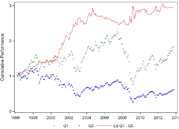
Figure 5. Performance of stock portfolios sorted on log variance risk premium
This figure presents the performance of the two extreme quintile portfolios and of a long-short low minus high log variance risk premium portfolio. The dotted lines represent the portfolio value of on an equally-weighted portfolio of stocks, rebalanced at the end of each month based on their log variance risk premium. The green dots represent the low log variance risk premium portfolio, while the blue dots represent the high log variance risk premium portfolio. The solid orange line represents the long-short portfolio. Stocks with the lowest log variance risk premium are allocated to portfolio Q1 while stocks with the highest log variance risk premium are allocated to portfolio Q5. The LS Q1-Q5 portfolio is a zero net investment portfolio, long on portfolio Q1 and short on portfolio Q5.
We find a negative relation between log variance risk premium and future returns. Though the average returns are not significantly different from zero in any of the quintile portfolios, a zero net investment portfolio, long on the stocks with low log variance risk premium and short on the high log variance risk premium stocks, shows a significant positive monthly return of 0.51% and a significant monthly Carhart of
10 Note that Han and Zhou (2011) define the variance risk premium as our definition multiplied by
(-1). Additionally, they use the predicted realized variance instead of the actual realized variance in each month.
22 0.64%. In line with this, the annualized Sharpe Ratio of this portfolio is 0.38, with an annualized Certainty Equivalent of 4.43%, substantially above the average annualized risk free rate during this period of 2.66%. Comparatively, Han and Zhou (2011), achieve a 2.86% monthly significant Carhart alpha (though their sorting variable is different). Figure 5 shows the cumulative performance of the extreme quintile and long-short portfolios, displaying the superior performance of the long-long-short strategy.
V. Option-implied betas
Following Buss and Vilkov (2012b), we now test whether stocks sorted at the end of the month in quintile portfolios by option-implied market betas may show significant difference in next-month returns. One would expect, based on previous literature, that these option-implied betas displayed future returns consistent with the expected risk-return relation.
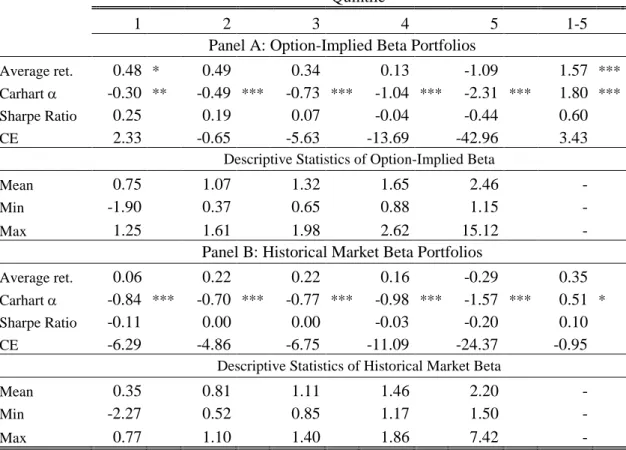
Table VI. Average stock return of option and historical market beta sorted portfolios
This table presents portfolio performance measures for quintile portfolios based on the option-implied and historical market betas of the stocks in our sample. Quintile portfolios are formed at the end of each month t-1, based on the option-implied beta for the next month and on historical market beta of the past 60 consecutive observations. Returns are the equally weighted average monthly return of the stocks in each quintile portfolio for month t. Please refer to Table V for variable and statistical description.
Quintile
1 2 3 4 5 1-5
Panel A: Option-Implied Beta Portfolios
Average ret. 0.48 * 0.49 0.34 0.13 -1.09 1.57 *** Carhart -0.30 ** -0.49 *** -0.73 *** -1.04 *** -2.31 *** 1.80 *** Sharpe Ratio 0.25 0.19 0.07 -0.04 -0.44 0.60
CE 2.33 -0.65 -5.63 -13.69 -42.96 3.43
Descriptive Statistics of Option-Implied Beta
Mean 0.75 1.07 1.32 1.65 2.46
-Min -1.90 0.37 0.65 0.88 1.15
-Max 1.25 1.61 1.98 2.62 15.12 -
Panel B: Historical Market Beta Portfolios
Average ret. 0.06 0.22 0.22 0.16 -0.29 0.35
Carhart -0.84 *** -0.70 *** -0.77 *** -0.98 *** -1.57 *** 0.51 * Sharpe Ratio -0.11 0.00 0.00 -0.03 -0.20 0.10
CE -6.29 -4.86 -6.75 -11.09 -24.37 -0.95
Descriptive Statistics of Historical Market Beta
Mean 0.35 0.81 1.11 1.46 2.20
-Min -2.27 0.52 0.85 1.17 1.50
23 As seen in Table VI, our average return shows a negative relation with beta. In fact, by forming, at the end of each month, a portfolio with the 20% highest beta stocks, we obtain average negative returns on our time series. More so, the relation between relative beta and future average return appears to be negative. Not only does this happen for option-implied betas but also for historical market betas.
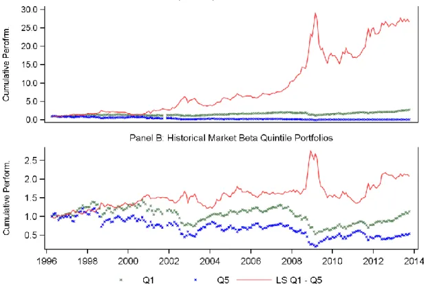
Contrarily to what would be seen as sensible for an investor, we present the performance of a zero net investment portfolio, long on the low beta stocks and high on the high beta stocks. This portfolio shows surprisingly good performance, with a significant average monthly return of 1.57%, a significant Carhart of 1.80 and a Sharpe Ratio of 0.17. Figure 6 shows the cumulative performance of the extreme quintile and long short beta-sorted portfolios. The striking difference in performance between the two long-short portfolios is attributed to the stable spread between Q1 and Q5 and also because of the consistent poor performance of the Q1 portfolio.
Figure 6. Performance of stock portfolios sorted on option-implied and historical beta
Each panel in this figure presents the performance of the two extreme quintile portfolios and of a long-short low minus high beta portfolio, where in Panel A option-implied beta sorted portfolios are shown, while in Panel B historical market beta sorted portfolios are shown. The dotted lines represent the portfolio value of on an equally-weighted portfolio of stocks, rebalanced at the end of each month based on their corresponding beta. The green dots represent the low beta portfolio, while the blue dots represent the high beta portfolio. The solid orange line represents the long-short portfolio. Stocks with the lowest beta are allocated to portfolio Q1 while stocks with the highest beta are allocated to portfolio Q5. The LS Q1-Q5 portfolio is a zero net investment portfolio, long on portfolio Q1 and short on portfolio Q5.
24 We suggest two hypotheses for the counter intuitive results we obtain for the option-implied betas. Firstly, it could come from the monthly implementation of the Buss and Vilkov (2012b) methodology. Namely, the usage of monthly correlations, given that we only use 60 observations for our historical measure, may cause this technique to be ineffective. Secondly, we consider possible that our sample may be significantly reduced, as a result of the database matching and the need for 60 month past correlation for beta calculation.
VI. Return prediction using option-implied information
In the previous sections, our results have hinted at the predictive power of both the log variance risk premium and the option-implied beta (despite in a counterintuitive sign). We now test the explanatory and predictive power of these two variables, alongside with historical Carhart betas. For this purpose, we use the standard Fama-Macbeth regressions to test whether these factors are significantly priced across our cross section of stocks and along the time period of our sample.11
This methodology is used to simplify a potentially complex panel data problem. First, the loadings of each asset pricing factor are calculated for each security, for each month. In our case, these loadings are the log variance risk premium, the option-implied beta, and the historical Carhart betas. Then, returns of all securities are regressed on those loadings for a particular month t (i.e. cross-sectionally), generating a coefficient which describes the premium associated with each factor loading, as in Equation (11).
(11)
This procedure is repeated for all months, until we have coefficient estimates for each asset pricing factor for all months. Finally, each time series of the coefficient estimates is treated individually and its mean and Newey-West standard error are calculated, in our case using a lag of one month, in order to test the average premium associated with each factor during the sample period.
11
We run the Fama-Macbeth regressions by using and adapting a SAS research macro kindly made available on the Wharton Research Distribution Services.
25 We run Fama-Macbeth regressions of the returns of month t and t+1 to test both explanatory and predictive power of the pricing factors in month t, respectively. We further restrict the sample into the S&P 500 constituents.
A. Predictive regressions
By running Fama-Macbeth regressions of month t on t-1 factors, we can assess whether our option-based factors are priced in the market. In Tables VII and VIII we present results for the whole sample and for the S&P 500 constituents, respectively.
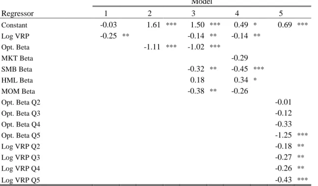
Through the analysis of Table VII, which includes all stocks in our sample, we can take several conclusions. With models 1 and 2 we can see that the individual pricing of the log variance risk premium and the option-implied beta is negative. This confirms the initial findings of Sections IV and V. Additionally, since the returns are expressed as natural logarithms and so is the log variance risk premium, we can interpret the coefficient as an elasticity. Consequently, in model 1, an increase of 1% in the log variance risk premium leads to a reduction of 0.25% in next month’s return. Note that difference between a percentage increase and percentage points of returns. The constant in model 1 is not statistically significant, which suggests a good explanatory power of the log variance risk premium. Nevertheless, we need global significance measures to assess this claim.
In model 3, by combining these regressors with historical betas, we see that their coefficients decrease, without losing statistical significance. The added variables, the
SMB, HML and MOM betas have different impacts. Both the SMB and the MOM factors
are negatively and significantly priced, while the HML factor is not significantly different from zero and has a positive coefficient.
We do not simultaneously include the option-implied beta and its historical counterpart in the model due to a potential problem of multicolinearity (which could be suggested by Figure 1). In model 4, we substitute the option-implied beta by the historical one and we see that it holds no predictive power. The SMB beta increases its negativity and significance, while the MOM beta loses the latter. This model choice must be economically motivated in a sense, as significance may fluctuate depending on the independent variables included. Additionally, an interesting note is that the log variance risk premium maintains its significance and coefficient value.
26 To continue the line of reasoning of the previous sections, we include dummies signaling to which quintile of option-implied beta and log variance risk premium a stock belongs to in a given month. These coefficients should be interpreted as the incremental next month return of a stock in each of the quintiles relative to the lowest quintile stocks. The results confirm two aspects of our previous analysis. First, the option implied betas quintiles do not show large differences except when comparing the smallest and largest quintile of stocks. Secondly, it confirms, now through the use of quintiles and again with statistical significance, the negative relation between log variance risk premium and future returns.
Table VII. Fama-Macbeth predictive return regressions for all stocks
This table presents the coefficients for different model configurations of Fama Macbeth regressions of next month returns on end-of-month factors from the current month for all stocks in our sample. Standard error calculated according to Newey and West (1987) with one lag autocorrelation. The null hypothesis tested is that the average coefficient equals zero. *, **, and *** denote a 10%, 5%, and 1% or lower p-value of the test statistics, respectively. Please refer to the beginning of Section VI for an explanation of how the presented coefficients are estimated.
Model Regressor 1 2 3 4 5 Constant -0.03 1.61 *** 1.50 *** 0.49 * 0.69 *** Log VRP -0.25 ** -0.14 ** -0.14 ** Opt. Beta -1.11 *** -1.02 *** MKT Beta -0.29 SMB Beta -0.32 ** -0.45 *** HML Beta 0.18 0.34 * MOM Beta -0.38 ** -0.26 Opt. Beta Q2 -0.01 Opt. Beta Q3 -0.12 Opt. Beta Q4 -0.33 Opt. Beta Q5 -1.25 *** Log VRP Q2 -0.18 ** Log VRP Q3 -0.27 ** Log VRP Q4 -0.26 ** Log VRP Q5 -0.43 ***
Contrasting these findings with those obtained when limiting the sample to the S&P 500 constituents, we lose nearly all the significance of the asset pricing factors (Table VIII). Consequently, we can state that the past log variance risk premium is not priced for this part of the sample, nor is the option implied beta. Nevertheless, the signs stay the same, with some differences in Carhart betas and option beta quintiles.
27
Table VIII. Fama-Macbeth predictive return regressions for S&P 500 stocks
This table presents the coefficients for different model configurations of Fama Macbeth regressions of next month returns on end-of-month factors from the current month for S&P 500 constituents in our sample. Please refer to Table VII for statistical description and to the beginning of Section VI for an explanation of how the presented coefficients are estimated.
Model Regressor 1 2 3 4 5 Constant 0.57 1.18 *** 1.09 *** 0.52 ** 0.73 *** Log VRP -0.18 -0.13 -0.20 ** Opt. Beta -0.47 -0.50 MKT Beta -0.03 SMB Beta 0.10 0.03 HML Beta 0.08 0.08 MOM Beta -0.13 -0.06 Opt. Beta Q2 0.18 Opt. Beta Q3 0.18 Opt. Beta Q4 0.13 Opt. Beta Q5 -0.17 Log VRP Q2 -0.19 * Log VRP Q3 -0.16 Log VRP Q4 -0.10 Log VRP Q5 -0.29 * B. Explanatory regressions
Regarding the contemporaneous explanatory power of our option-implied variables, we see by Table IX and Table X that results are statistically significant for both the full sample and the S&P 500 subsample, unlike those of the predictive regressions. Regarding Table IX, we see that the log variance risk premium now has a higher coefficient in absolute terms and remains statistically significant. This implies that the elasticity mentioned before is now higher in absolute terms as well. In this case, a stock with a 1% higher variance risk premium in a given month t will have -1.08% lower returns in that same month t, according to Model 1. The value of this coefficient drops to -0.84% and -0.82% as more dependent variables are added to the specification. The option-implied beta maintains its counterintuitive sign and also its statistical significance, but again with a larger coefficient in absolute terms. Interestingly, the historical Carhart betas, on their turn, show no statistical significance in explaining contemporaneous returns.
28
Table IX. Fama-Macbeth explanatory return regressions for all stocks
Please refer to Table VII for statistical description and to the beginning of Section VI for an explanation of how the presented coefficients are estimated.
Model 1 2 3 4 5 Constant 0.33 3.78 *** 3.74 *** 0.94 *** 1.48 *** Log VRP -1.08 *** -0.84 *** -0.82 *** Opt. Beta -2.66 *** -2.59 *** MKT Beta -0.40 SMB Beta 0.18 -0.28 HML Beta -0.25 0.09 MOM Beta -0.65 * -0.28 Opt. Beta Q2 -0.36 ** Opt. Beta Q3 -0.84 *** Opt. Beta Q4 -1.62 *** Opt. Beta Q5 -3.93 *** Log VRP Q2 0.21 * Log VRP Q3 0.50 *** Log VRP Q4 0.65 ** Log VRP Q5 -0.94 *
Dummies for both the option-implied beta and the log variance risk premium show statistical significance. Those of option-implied betas show a decreasing pattern of returns for greater betas, again the counterintuitive relation we found. The log variance risk premium, quite differently, show an increasing relation with returns for larger quintiles except for Q5, which hints at two possible hypothesis. Either these marginal coefficients for the log variance risk premium dummies are suffering from model misspecification or the negative coefficient associated with the log variance risk premium in the remaining models may be driven by stocks in the last quintile. The same analysis is valid for the S&P 500 segment, suggesting that the option-implied information is more significant for explanatory regressions rather than predictive ones in the large market capitalization segment.