Predictable Dividends and Returns
Job Market Paper
Ruy Ribeiro
1Graduate School of Business
University of Chicago
November, 2002
1Ph.D. Candidate in Finance. Email: [email protected]. I am grateful to George
Abstract
The conventional wisdom is that the aggregate stock price is predictable by the lagged
price-dividend ratio, and that aggregate price-dividends follow approximately a random-walk. Contrary to
this belief, this paperfinds that variation in the aggregate dividends and price-dividend ratio is
related to changes in expected dividend growth. The inclusion of labor income in a cointegrated
vector autoregression with prices and dividends allows the identification of predictable variation in
dividends. Most of the variation in the price-dividend ratio is due to changes in expected returns,
but this paper shows that part of variation is related to transitory dividend growth shocks.
Moreover, most of the variation in dividend growth can be attributed to these temporary changes
in dividends. I also show that the price-dividend ratio (or dividend yield) can be constructed as
the sum of two distinct, but correlated, variables that separately predict dividend growth and
returns. One of these components, which could be called the expected return state variable,
1
Introduction
Are innovations to the aggregate stock price related to changes in expected future aggregate
dividend growth? Theoretically, the aggregate stock price is the value of the expected future
dividends discounted with a constant or time-varying discount rate. In the case of constant
ex-pected returns, the present-value model says that all variation in stock price is due to changes in
current dividend growth and expected future dividend growth. If the discount rate is constant, a
change in the aggregate price-dividend ratio is caused by a change in expected dividend growth.
Nevertheless, the empirical literature cannot identify the key prediction of this simple present
value model. Almost all variation in the aggregate stock price and price-dividend ratio is
associ-ated with changes is expected returns. Moreover, variation in dividends that does not coincide
with a change in current stock price does not add more information about the future evolution of
dividends, but predicts the future path of stock prices. Hence, the conventional wisdom is that
aggregate dividends are close to random-walks and that the aggregate stock price is predictable
by the lagged price-dividend ratio. Contrary to this belief, this paper finds that variation in
dividends and price-dividend ratio is related to changes in expected dividend growth.
The purpose of this paper is to present an analysis of dividend growth predictability and its
relation to stock prices. Most of the empirical literature on time-series predictability has focused
on the variability of expected returns, because of the strong evidence that stock prices do not
predict dividends1. For instance, Cochrane (1994) shows that a permanent dividend growth
shock effectivelly explains all variation in dividend growth and a small fraction of the variance
in stock price growth. The remaining variation in aggregate stock price growth is explained by
changes in expected returns. A large literature has confirmed the absence of dividend growth
predictability and the economic importance of the variability in expected return2. On the other
hand, the statistical significance of the expected return predictability has also been questioned
by recent work3.
1Other contemporaneous papers present empirical evidence that dividends are predictable. Lettau and
Lud-vigson (2002) show that there is predictability in dividends growth, but they do not find that innovations to price-dividend ratio convey information about future dividends. Ang and Bekaert (2002) also claim that divi-dends are predictable if different data sets are considered.
2For example, Campbell and Shiller (1988), Campbell (1991), Cochrane (1991), Lamont (1994), Cochrane
(1997), Campbell and Shiller (2001), Lewellen (2001).
The empirical literature on the present-value models has identified the presence of two shocks
to prices and dividends: an expected return shock and a permanent dividend growth shock.
In this paper, I identify a transitory dividend growth shock, which could be interpreted as an
expected dividend growth shock. I augment the conventional vector autoregression to account
for the existence of broadly defined cash flow shocks. Specifically, I include the aggregate labor
income in the cointegrated vector autoregression of aggregate stock price and dividends4. This
allows me to identify temporary changes in dividends, since they are not accompanied by changes
in labor income and stock price. The reason could be that the shocks to the aggregate cashflow
in the economy do not have a uniform and simultaneous impact on cashflows to inputs like labor
and capital. It is reasonable to believe that stock prices may not react to changes in dividends
that are not expected to persist. I present empirical evidence that this expected dividend shock
can explain an economically significant fraction of the variance of the dividend growth and the
variance of the innovations to the price-dividend ratio.
In a recession, dividends may fall more than labor income. Dividends will then rise more in the
recovery. The low dividend-labor income ratio in the recession forecasts high subsequent dividend
growth. If this were the only effect, the price-dividend ratio would be higher in recessions.
However, in the depth of the recession, expected excess returns are also high. Even though
dividends are expected to grow at a faster rate, the price-dividend ratio may not be much affected.
In this simple situation, the expected dividend growth and the expected return are perfectly
correlated and the correlation is motivated by business cycle fluctuations. Even if they are less
than perfectly correlated, the price-dividend ratio may not forecast dividend growth, because
of the higher variance of the expected return shock. Conditioning on an enlarged information
set that includes labor income, I can show that variation in the price-dividend ratio is due to
dividend growth. Even if the shocks are orthogonalized, I can still show that a significant fraction
of the price-dividend variance is explained by dividend growth.
This evidence on dividend growth predictability apparently contradicts the usual results of
regressions that use lagged (log) price-dividend ratios to predict future prices (or returns) and
the statistical problems with the commonly used predictive regressions.
4Other cashflow data could have been used here such as the national income, but this measure also includes
dividends. In these regressions, lagged price-dividend ratios tend to predict returns (and changes
in stock price) but not dividend growth. However, I show that even if price-dividend contains
information about variation in expected dividend growth, it may not predict future dividends.
In fact, the aggregate price-dividend ratio is the sum of two variables that separately predict
dividends and returns. Once the price-dividend ratio (or dividend yield) is decomposed into
these two variables, it is possible to identify the two regressors that predict future dividend
growth and returns. I also show that one of these forecasting variables, the expected return
state variable, predicts returns better that the price-dividend ratio (or dividend yield). Even if
these two variables were completely independent, the price-dividend ratio would not necessarily
be able to predict future dividend growth, since the price-dividend ratio could be described as
the relevant independent variable plus measurement error represented by the expected return
variable. This measurement error problem can make the regression coefficient on lagged the
price-dividend ratio statistically insignificant. Since these two state variables are correlated, the
coefficient on the lagged price-dividend ratio may have the unexpected sign, exactly the result
found in the empirical literature.
The paper is organized as follows. Section 2 introduces the data and explores the past results
found in return and dividend growth predictive regressions. Section 3 presents the estimated
vector autoregressions and shows the benefits of the inclusion of labor income to the econometric
model. Section 4 shows the results of the price-dividend ratio variance decomposition including
labor income in the information set. Section 5 proceeds with the identification of the
orthogonal-ized shocks, and presents the results of the respective variance decompositions which show again
that dividend growth affects price-dividend ratio. Section 6 analyzes the results with univariate
regressions in the light of the more general approach presented in this paper. Section 7 concludes.
2
Predictive Regressions
This section presents the results with the commonly used return and dividend growth predictive
regressions and a discussion about the reasons why dividend growth does not seem to be
pre-dictable in these regression. I will return to this discussion in section 6, after I introduce in detail
First, I briefly describe the data. The dividends and aggregate stock price come from the NYSE
data available in the CRSP files. The annual sample begins from 1929 and ends in 2000. I use
the implicit deflators from the national accounts to calculate the real values for the variables.
The log real aggregate stock price, pt, is the natural logarithm of the real value-weighted stock
index calculated with all the shares in the NYSE at the end of the period. This stock price index
is calculated as the accumulated return without dividend reinvestment. The log real aggregate
dividenddtis built from the stock price index and the information about dividend yield obtained
with the annual return and the annual return without dividends. I constructed an earnings series
using the information about earnings per share from the S&P Composite Index. The earnings
variable was calculated considering the ratio between earnings and dividends calculated using
only the stocks in the S&P500. Besides the stock market data, the real per capita labor income
and consumption data were obtained from the national accounts. I express these variables in
terms of their natural logarithm and are represented by lt and ct. Appendix A has detailed
definitions of the data and methodology used to calculate these variables.
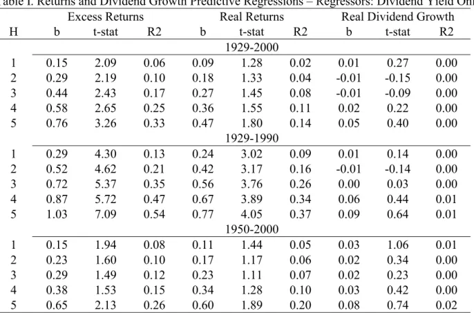
Table 1 presents the results with the most commonly used predictive regressions of excess
returns, real returns and real dividend growth on the lagged dividend yield. Three different
samples are considered: 1929-2000, 1929-1990, and 1950-2000. If I exclude the nineties from the
sample, both excess returns and real returns are predicted by the dividend yield. This result
holds for different horizons where the accumulation of returns or growth rates varies from one
to five years. The inclusion of the nineties makes the real returns statistically unpredictable.
If only the last fifty years of data are considered, the predictability becomes even weaker. On
the other hand, the real dividend growth does not seem to be predictable for any sample choice.
Since high prices could imply that there is expectation of higher future dividends, the sign of
the coefficient is expected to be negative in this regression. But the coefficient on the lagged
dividend yield rarely has the predicted sign.
A simple view of this commonly used predictive regressions is that the dividend yield (or
price-dividend ratio) is related to the mean of the processes that govern stock returns and price-dividend
growth. However, these regressions may not reveal dividend predictability if the expected returns
are extremely volatile. Since the innovations to expected dividend growth and expected returns
price-dividend ratio what is related to news about expected returns or expected price-dividend growth.
It is necessary to introduce more information into the traditional autoregression, because the
price-dividend ratio may only summarize the contribution of two distinct variables that may
individually explain expected dividend growth and expected returns.
The objective is to identify the expected dividend component of the price-dividend ratio
variation. The main idea of this paper is that prices may react to news about cash flows that
do not impact dividends immediately, or that there may be changes in dividends which are
temporary because they are not instantly followed by other cash flows. These additional cash
flows should not be perfectly related to the stock market cash flow data, but they should share
a common growth component. If this is true, stock market information is not enough to identify
these particular innovations to aggregate stock price and aggregate dividend. Therefore, the
vector autoregression that describes the evolution of prices and dividends should include other
variables that may reveal both the temporary and permanent components of dividends. Stock
prices may react to news to these other cashflows that are not directly related to the stock market
(for example, private companies’s profits, labor income, etc.), if market believes that these news,
whether good or bad, will impact dividends later on. Future dividends will be affected if the
news are related to the common stochastic growth component.
A natural candidate for this additional variable is aggregate labor income, since it accounts for
the largest share of the total income. Consequently, it may be extremely important to consider
the effect of the existence of a long-run relation between (log) labor income and (log) dividends,
even when analyzing the relation between prices and dividends. It is reasonable to assume that
log labor income and log dividends are cointegrated with a unitary cointegrating vector5, because
we may believe that the ratio of dividends to labor income is stationary. This property is related
to the idea that the share of dividends to the total income is stationary. I will also consider the
assumption that the price-dividend ratio is stationary, which is more common in the literature.
The ratio of consumption to dividends could also be used to predict future dividend growth.
However, the changes in this ratio could also be related to changes in expected returns. Table 2
shows results of dividend growth and excess returns predictive regressions on different candidates
for dividend growth predictor. I consider the labor income-dividend ratio, earnings-dividends
ratio and consumption-dividend ratio as possible predictors. Earnings-dividends ratio does not
predict future dividend growth. Since the consumption-labor income ratio has been very stable
in the last fifty years, both labor income-dividend ratio and consumption-dividend ratio predict
future dividends with similar performance. Using full sample, the consumption-dividend ratio
tends to perform better, since the labor income-dividend ratio is more variable in the beginning
of the this sample. Nevertheless, the consumption-dividend ratio also predicts excess returns6,
especially at long horizons. The consumption-dividend ratio explains an economically significant
fraction of the variation in expected return. In the five-year horizon regressions, the r-squared
of the regression of excess returns on the lagged consumption-dividend ratio is 0.24 (0.21 if
sample is 1950-2000), while the r-squared with labor income-dividend ratio is only 0.08 (0.10).
The coefficients of return regressions on these lagged variables is statistically more significant
when the consumption-dividend ratio is used. Therefore, the labor income-dividend ratio tends
to predict mostly dividend growth, while consumption-dividend ratio predicts both expected
returns and dividend growth7. I choose the log labor income-dividend ratio, since the objective
is to identify the determinants of variation in price-dividend ratio and not to find the best
predictor of dividend growth.
3
Vector Autoregressions
All these series in levels are integrated of order one and they may share a common stochastic
growth component. In accordance with the Granger representation theorem, the vector
autore-gressions should include the first differences of these series and the lagged cointegrating errors
in the error correction form. Hereafter I consider only two possible candidates for cointegrating
6I performed the same calculations with real returns, but they are excluded since the qualitative results are
similar.
7Additionally I regress dividend growth, excess returns and real returns on the lagged values ofc
t−lt and lt−dtsimultanueously. The idea is that(ct−dt) = (ct−lt) + (lt−dt)can capture the effect of changing expected
returns and changing expected dividend at the same time, but(ct−lt)mostly captures expected returns (Santos
and Veronesi (2001), while the remaining part captures the variation in expected dividend growth. The dividend predictive regression shows that only(lt−dt)predicts dividend growth, since(ct−lt)is statistically insignificant.
At the same time, the real returns regression shows that(ct−lt)predicts returns, while(lt−dt)is statistically
and economically insignificant. The correlation between(ct−lt) and(lt−dt)is only 8.6%. These particular
vectors. I assume that the log price-dividend ratio and the log dividend-labor ratio are
station-ary. This assumption is equivalent to the existence of two unitary cointegrating vectors. The
notation for the additional terms are pt−dt anddt−lt , but both log ratios are demeaned and
have the interpretation of cointegrating errors.
Hence, the econometric model is:
yt=A+B(L)yt−1+Cxt−1+ut (1)
where the vector yt = [∆lt ∆pt ∆dt]T and xt = [pt−dt, dt−lt]. The vector of errors ut has
constant variance-covariance matrixΣu. In the specification with earnings, dt is replaced byet.
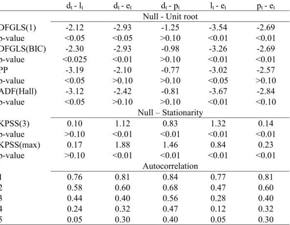
Taking as given the available evidence that all the variables in levels are I(1), I test the
existence of the cointegration between different pairs of variables. Table 3 provides unit root
tests for the log ratios of pairs of variables, which can be interpreted as cointegration tests, if I
only allow unitary coefficient. The tests based on unit roots as a null hypothesis show that the
bivariate relations between all the cash flow variables dividends, earnings and labor income
-seem to be stationary, since it is possible to reject the existence of unit roots in all cases. This
result can be confirmed with the tests based on stationarity as a null hypothesis in the case of
the dividend-labor income ratio. The autocorrelations also decay much more rapidly in the case
of dividend labor income ratio. However, it is more difficult to claim stationarity in the case of
the price ratios.
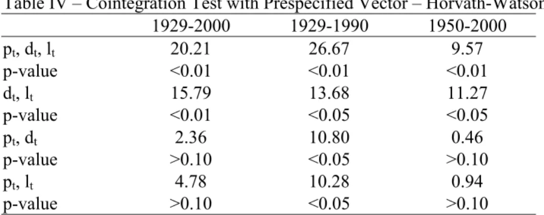
Table 4 presents trivariate and bivariate cointegration tests that restrict the attention to
unitary cointegrating vectors8. I test a null hypothesis that there is no cointegration against
an alternative hypothesis that the variables are cointegrated with unitary vectors, which are
supposed to be known. These tests use the procedure in Horvarth and Watson (1995). The
advantage of imposing known cointegrating vectors is that the test becomes more powerful. In
the case where all coefficients are predetermined, the Horvarth-Watson test is the standard Wald
test for the presence of the cointegrating errors in the system. The test rejects the null of no
cointegration when stock price, dividends and labor income are considered. The Horvath-Watson
8Alternatively, I followed the Johansen procedure to obtain the estimates of the cointegrating vectors for two
test was applied to pairs of variables and the only pair to reject the hypothesis of no cointegration
were labor income-dividends. Figure 1 shows the plot of the log dividend-labor income and log
dividend-price ratio. The visual analysis of the data shows that the log dividend-labor income
seems to be stationary.
I present the results of the vector autoregression estimation. First, I analyze regressions
without lags, which is the common approach of predictive regressions. This representation is
possibly a restricted version of the true VAR model. If I only included price and dividends
equations in the system, both Akaike and Schwartz model selection criteria would recommend
the exclusion of lag terms. The main reason for inclusion of lags in the system is the labor income
equation, since the log growth rate of labor income seems to depend on its past realization.
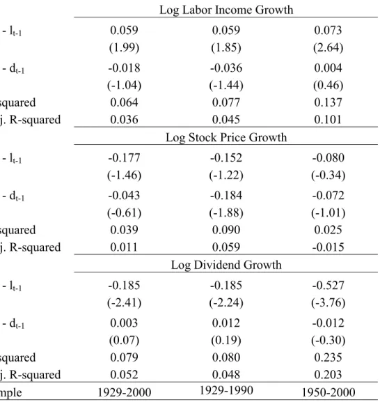
Table 5 presents the results of the regression without lags for three time periods which are
the full sample (1929-2000) and two additional sub-samples (1929-1990 and 1950-2000). I show
that dt−lt predicts the future changes in both log labor income and log dividends. This result
is statistically significant in all samples and both equations. The economic effect of the lagged
dt −lt is more relevant in the case of the dividend equation, since the speed of reversion is
considerably larger and dividends tend to revert much more quickly to the long-run relation
between dividends and labor income. The speed of mean reversion of dividends to this long-run
relation is the coefficient on the lagged dt−lt. It varies from -0.185 to -0.527 depending on the
sub-sample used. By comparison, the same coefficient for labor income equation is between 0.059
and 0.073 across sub-samples. The stock price equation shows that the log price-dividend ratio
predicts future changes in log prices, but it is not clearly statistically significant. The lagged
dividend-labor income ratio does not explain much of the variation in stock price growth. The
log price-dividend ratio does not predict future dividend growth.
The basic result of these autoregressions does not change even after adding lags. The
statis-tical significance of the coefficients is affected due to the possible collinearity of the additional
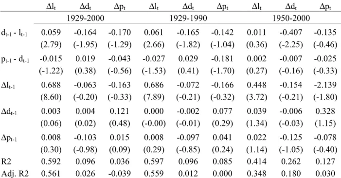
regressors. Table 6 shows the results of the vector autoregression of order one. This is the order
of autoregression which is suggested by the Schwartz criterium. The only variable that seems to
be explained by its own lag is the log labor income growth. The coefficient on the lagged log
dividend-labor income ratio in this equation becomes smaller, and it is very close to zero in the
as in the no-lag regression on the evolution of future changes in log dividends. Consequently,
dividend growth appears to be responsible for most of the adjustment to the long-run
equilib-rium relation between dividends and labor income. The changes in log prices are still predictable
by the lagged log price-dividend ratio. In general, the significance of the coefficients decreases
because of the change in standard errors.
4
Price-Dividend Ratio Decomposition
The price-dividend ratio summarizes information about conditional expected dividend growth
and conditional expected returns. Since the inclusion of labor income may reveal transitory
variation in dividend growth rate, the variance of the expected dividend growth could increase.
Following Campbell and Shiller (1988), the demeaned log price-dividend ratio can be represented
as
pt−dt=Et
∞
X
j=1
ρj−1
(∆dt+j −rt+j). (2)
Given the proposed VAR, I can compute the conditional expectation of both the discounted
dividend growth and discounted return:
sd,t =E X∞
j=1
ρj−1 ∆dt+j
¯ ¯ ¯ ¯ ¯ ¯zt
, sr,t=E X∞
j=1
ρj−1
rt+j
¯ ¯ ¯ ¯ ¯ ¯zt
(3)
and they should satisfy the following restriction
pt−dt=sd,t−sr,t. (4)
The information setzt may include the cointegrating errors and all the variables with
respec-tive lags:
zt = [∆dt,∆dt−1, ...,∆lt,∆lt−1, ...,∆pt,∆pt−1, ..., lt−dt, pt−dt]T (5)
and has a first-order VAR representation
where the matrix D is composed of the elements of the matrices B and C and uet is also a
combination of the elements of the error vector ut in equation (1).
Both conditional expectations depend linearly on the vector zt :
sd,t=E X∞
j=1
ρj−1 ∆dt+j
¯ ¯ ¯ ¯ ¯ ¯zt
=e∆dtD(I−ρD) −1
zt =Sdzt (7)
sr,t =E X∞
j=1
ρj−1
rt+j
¯ ¯ ¯ ¯ ¯ ¯zt
= (ρept−dtD+e∆dtD−ept−dt)(I−ρD)−1
zt =Srzt (8)
whereex is a row vector with 0’s everywhere and 1 for one particular element, satisfying the
con-ditionex.zt=x. The row vectorsSd andSr represent the loadings of the conditional expectation
on each of the elements of the information setzt and satisfy the condition (Sd−Sr).zt =pt−dt.
If the labor income information is included,Sdalways has a positive loading on the term lt−dt.
All the other loadings are very small, except for the lagged labor income growth if thefirst-order
lags are included. But most of the variation in the conditional expectation of the discounted
dividend growth is due to changes in the labor income-dividend ratio. Figure 2 depicts the
val-ues for sd,t and sr,t estimated for the sub-sample 1950-2000 assuming that (1) is a cointegrated
VAR(1). The results are not sensitive to alternative specifications.
The variance of the price dividend ratio could be decomposed into three terms: the variance
of each one of the conditional expectation terms and their covariance:
var(pt−dt) =var(sd,t) +var(sr,t)−2cov(sd,t, sr,t). (9)
If labor income is included, the terms var(sd,t) and cov(sd,t, sr,t) increase significantly in
absolute terms. The increase in the first term is consistent with the idea that dividends are
predictable, but the conditional expectation of the discounted dividend growth seems to be
positively correlated with the conditional expected returns. Therefore, the covariance term also
increases. Table 7 presents the results of the variance decomposition in equation (9) and the
correlation between sd,t and sr,t. If labor income growth and labor income-dividend ratio are
excluded from the process (1), the fraction of the total variance that is explained by dividend
income is include, this number can reach 32.3%. There is a simultaneous increase in the covariance
term, which is due to the possible correlation between expected returns and expected dividend
growth. But the correlation between these two variables is never above 60%.
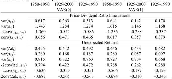
A similar result holds if the variance of the innovation to the price-dividend ratio is
decom-posed into the variance of the innovations to the conditional expectations sd,t andsr,t and their
covariance:
var((Et−Et−1)(pt−dt)) = var(Sduet) +var(Sruet)−2cov(Sduet, Sruet). (10)
The top panel of table 8 shows the results of this variance decomposition. Interestingly, the
contribution of dividend growth is even higher with this alternative variance decomposition. The
correlation between Sduet and Sruet is not much different than the one obtained in the previous
variance decomposition.
It is also possible to decompose the variance of the unexpected return, which is defined as:
rt−Et−1rt = (Et−Et−1)∆dt+ (Et−Et−1) X∞
j=1
ρj∆dt+j −
∞
X
j=1
ρjrt+j
(11)
var(rt−Et−1rt) = var(e∆dtuet) +var(ρSduet) +var(ρSruet) + 2cov(e∆dtuet,ρSduet)
−2cov(e∆dtuet,ρSruet)−2cov(ρSduet,ρSruet). (12)
Because of the contemporaneous correlation between returns and dividends, the first term
of this variance decomposition become economically significant. The bottom panel of table 8
also shows that the dividend growth conditional expectation contributes to the variance of the
unexpected returns.
5
Impulse Response Functions
The Campbell-Shiller decompositions above are not based on orthogonalized components. In
this section, I identify orthogonalized shocks that affect the time-series behavior of the aggregate
long-run properties. The procedure has two steps. First, a transformation is applied to the VAR
innovation vector is such a way that guarantees that these modified, but still unorthogonalized,
shocks have some desired long-run properties. After the first transformation, the shocks
can-not be interpreted as shocks to each one of the equations anymore, since they become linear
combinations of the original innovations. Second, the Choleski decomposition is applied to the
variance-covariance matrix of the modified shocks, since these modified shocks are not
necessar-ily orthogonal. Appendix B describes the two-step procedure used to calculate these impulse
response functions in more detail. Figures 3 to 8 present the impulse response functions of the
three variables to each one of the orthogonalized shocks. To avoid excessive information, I only
present the responses with full sample and the last fifty years of data, but similar results obtain
in other samples. I will name each of the shocks according to the economic interpretation that
best suits them.
Figures 3 and 4 depict the impulse response function of a permanent dividend shock. This
shock corresponds to a positive change to labor income, dividends and stock prices in a
combina-tion that guarantees that the initial change to dividends persists indefinitely. The small decrease
in the effect of the dividend innovation in the first years is due to the autoregressive component
in the labor income process and to the economically significant reversion of the dividend process
to the long-run equilibrium relation between labor income and dividends.
The response of the variable to a negative expected dividend shock is plotted infigures 5 and
6. This shock could also be interpreted as a transitory shock to dividends, since it is a positive
change to dividends that is not expected to fully persist in the future. In the sub-sample
1950-2000, this positive change in dividends is expected to completely disappear in the long run. In
most of the sub-samples, this change in dividends is accompanied with a small positive change to
stock prices, that will also disappear in the long run. The expected returns shock is essentially a
change in prices that has no immediate effect on dividends and labor income, as shown infigures
7 and 8. Therefore, stock prices exhibit reversion to the original level, which is determined by
these two cashflow variables.
It is evident that labor income has an important role in identifying the shocks to prices that
have information about future dividends. For example, a fraction of the good news in the labor
price increases. The aggregate stock price may increase if the financial market believe these
good news will affect dividends later. It is possible to create this type of shock by combining
a positive expected dividend shock (a temporary decrease in dividends) and a positive current
dividend shock (a positive and permanent innovation to stock price, dividends and labor income)
in certain proportions. This combination of shocks correspond to the situation where both labor
income and aggregate stock price increase without an immediate change in dividends. To my
knowledge, this type of shock has not been shown in the past literature. However, it is important
to verify whether the temporary shocks to dividends produce economically significant variation
in dividends and price-dividend ratios.
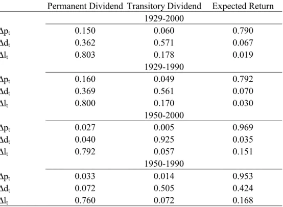
Table 9 presents the forecast error variance decomposition of stock price growth, dividend
growth and labor income growth in terms of the orthogonalized shocks: the expected return, the
transitory dividend growth and the permanent dividend growth shocks. The qualitative results
do not depend on the sample or the order of the autoregressions. I considered four different
samples: 1929-2000, 1929-1990, 1950-1990 and 1950-2000. A large share of the dividend growth
variance is related to temporary shocks to dividends. The calculations show that across the
used sub-samples at least 50.5% of the variance of log dividend growth can be attributed to
temporary dividend growth shocks. On the other hand, most of the variation in prices is driven
by changing expected returns. The temporary dividend growth shocks do not impact stock prices
significantly, but the permanent dividend shocks do.
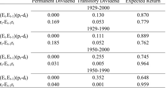
Cochrane (1994) has shown that almost all variation in price-dividend ratio is related to
changing expected returns. However, the calculations with the model that includes labor income
show that a fraction of this variation is due to changing future dividends. If the full sample is
used, the fraction of the variance of the unexpected changes in price-dividend ratio, as in equation
(10), that can be attributed to expected dividends is 13.0%, while expected returns explain the
remaining variation9. In the sub-sample 1950-1990, the contribution of expected dividend to
price-dividend ratio unexpected changes increases to 35.2%.
Campbell (1991) presented the variance decomposition for unexpected returns, which was
9The numerical calculation shows that the current dividend shock explains at most 0.5% of the price-dividend
presented in equation (11). In this formula, the summation of the dividend term start at j=0,
since a positive shock to current dividend affect returns instantaneously. Thus, the current
dividend shock should explain a significant part of the variance of unexpected returns. At the
same time, the importance of the expected dividend shock must decrease. Table 10 shows that
the contribution of the current dividends to the variance of unexpected returns can be as large
as 18.5% if the nineties are excluded from the sample. The inclusion of the nineties makes the
contribution of the expected return shock much larger. In the sample, 1950-2000, the expected
return shock explains basically all variation in unexpected returns, 96.4%. In the sample
1929-2000, only 5.3% of the variance is explained by the expected dividend shock. Similar results are
obtained for all the above decompositions, if earnings are used instead of dividends, as seen in
Table 11.
6
Predictive Regressions Revisited
In this section, I will focus on a simple VAR representation to better understand the effect of
the previous results on the estimation of predictive regressions. This section is not based on
any particular assumption about the orthogonalization of the VAR variance-covariance matrix.
I showed that part of the variation in price-dividend ratio is related to changes in expected
dividend growth, but this result seems to inconsistent with the predictive regression presented in
section 2. Here I show that this result is not inconsistent, because the price-dividend ratio is not
the variable that determines the mean of the dividend and stock price growth. Here I show that
the variation in price-dividend ratio or dividend yield may be determined by two state variables
that separately determine the evolution of dividends and returns. I will call these processes state
variables, since they summarize all the relevant information about expected dividend growth and
expected returns.
In order to present these ideas more clearly, I will focus on a restricted version of the model in
section 3. This model is a good approximation of the true representation under the assumption
that the lag of the variables do not provide relevant information about expected returns and
expected dividend growth. But the same conclusions are obtained under alternative specifi
returns and expected dividend growth respectively. Both of them follow a simple autoregressive
form and all variables are demeaned.
xt =bxt−1+δt (13)
yt =ayt−1 +θt (14)
Consequently, log returns and log dividend growth are driven by the following processes:
rt+1 =xt+εr,t+1 (15)
∆dt+1 =πyt+εd,t+1 (16)
I will also assume that labor income growth is not affected by any of the state variables.
∆lt+1 =εD,t+1 (17)
I showed previously that the log labor income ratio forecast dividend growth, but does not
seem to be directly related to expected returns. If the conditional expectation of the discounted
dividend growth is calculated, almost all the weight is given to the lagged labor income-dividend
ratio. Therefore, I will assume that
yt= (lt−dt) (18)
I can apply the approximate relation between the log price-dividend ratio and the discounted
difference between expected dividend growth and returns to obtain the following equation:
pt−dt = Et
∞
X
j=1
ρj−1(∆dt+j −rt+j) (19)
= π(lt−dt)
1−ρa − xt
1−ρb
Now the price-dividend ratio is determined by both state variables. It is also possible to
show that there are representations of returns, changes in log stock prices and dividend growth
rt+1 =xt+εD,t+1−ρ
δt+1
1−ρb (20)
∆pt+1 =
π[(1−ρ)a)]
1−ρa (lt−dt) +
[(1−b)]
1−ρb xt+εD,t+1− δt+1 1−ρb +π
θt+1
1−ρa (21)
∆dt+1 =π(lt−dt) +εD,t+1−θt+1 (22)
The stock return process is solely determined by the expected return state variable because of
the assumption in equation (15), but changes in log stock prices are also affected by the expected
dividend state variable. Consistent with the idea of the previous sections, three different shocks
affect all these variables. The shockεD,t+1 is the permanent dividend shock at time t+1, because
it affects stock price, dividend and labor income and it is persistent. The realization of the
shock δt+1 corresponds to the expected return innovation at time t+1. While θt+1 captures
the innovations to expected dividend growth or the temporary shock to dividends. Similar
representation can be found for the price-dividend ratio innovations.
pt+1−dt+1 =π
a(lt−dt)
1−ρa − bxt
1−ρb +π θt+1 1−ρa −
δt+1
1−ρb (23)
Therefore, it is possible to represent the unexpected shocks to returns and price-dividend
ratio as:
(Et+1−Et)rt+1 =εD,t+1−ρ
δt+1
1−ρb (24)
(Et+1−Et)(pt+1−dt+1) =π
θt+1 1−ρa −
δt+1
1−ρb (25)
which was the approach of the decomposition in the previous section.
The price dividend ratio is determined by two different state variables, but only one of
them predicts future dividend growth. If the variable that predicts dividend growth is correctly
identified, it is possible to identify the state variable that predicts returns. Let’s define the cash
flow and expected return state variables respectively as:
cft =π
(lt−dt)
ert=
xt
1−ρb (27)
and
pt−dt=cft−ert (28)
The expected return state variable is obtained using equation (19). The necessary parameters
are estimated using equations (14) and (16). I assume that ρ is equal to 0.96 in these
calcula-tions, but results are not sensitive to different choices. Similar state variables are obtained if a
cointegrated VAR(0) is estimated and the conditional expectations in section 3 are computed.
The following results are not specific to the order of the VAR. Future versions will include the
results with alternative specifications.
The basic idea is that the price-dividend ratio is a noisy variable for each one of the predictive
regressions. In the dividend growth predictive regression, it is expected that cft should predict
dividend growth. But the variable pt − dt is cft plus a measurement error. Since expected
returns are much more variable than the cashflow state variable, the measurement error is large.
Therefore, the coefficient of the dividend growth regression on the lagged price-dividend ratio
(or dividend-yield) is expected to be close to zero. If the cash flow and expected return state
variable are positively correlated, the coefficient can even have the unexpected sign. The same
logic could hold in the case of the return predictive regressions. Because the measurement error
problem is relatively less important, the coefficient will not necessarily be significantly biased.
However, returns become more forecastable if the expected return state variable is used instead
of the price-dividend ratio, independently of the assumptions for its identification..
Tables 12 and 13 report the results of return predictive regressions for one tofive-year horizons
with three different sets of regressors: dividend yield; expected return state variable; and both
expected return state variable and cashflow state variable. Table 12 presents results with the full
sample, while table 13 concentrates on the lastfifty years of available data. Each panel includes
regressions with excess returns and real returns as dependent variables. Panel A presents OLS
regressions of returns on the dividend yield, while panel B provides OLS regressions with the
expected return variable. For both excess returns and real returns, we see an increase in the
statistical significance of the regressor, when the expected return state variable is used. If the
regressions almost doubles. It is important to note that the increased statistical significance
of the regressor is due to a reduction of standard error when I use the expected return state
variable, since the coefficients tend to become smaller. The standard errors decrease in every
regression with the expected the return state variable for both samples. If the expected return
state variable is correctly identified, the addition of the cash flow (or expected dividend) state
variable should not impact the results.
Panel C of tables 12 and 13 provide OLS regressions with both state variables as regressors.
The cashflow state variable is always statistically insignificant. The coefficient estimate on the
expected return state variable is not economically affected in long horizons. The R-squared
does not change considerably if the cash flow state variable is added. The standard errors of
the expected return tends to increase, since these state variables have correlation of 0.30 in full
sample. Therefore, expected returns are more predictable than past literature showed, if one
focus on the expected return component of the dividend yield.
Tables 14 and 15 provide OLS predictive regressions of future dividend growth on three
different sets of regressors: dividend yield; cash flow state variable; and both cash flow state
variable and expected return state variable. Panel A shows the commonly used regressions of
dividend growth on the lagged dividend yield. Once again, I would expect a negative sign if
high prices indicated higher expected dividend growth, but coefficients are positive. Of course,
panel B in both tables shows that future dividends are predicted by the lagged cash flow state
variable. These results are much stronger if the sample 1950-2000 is considered. Panel C in both
tables shows that the inclusion of the expected return state variable does not affect the statistical
significance of the cash flow state variable.
7
Conclusion
This paper shows that there exists economically significant variation in expected dividend growth.
I find that changes in aggregate dividends that do not coincide with changes in labor income are
mostly short-lived. Hence, it is feasible to recognize the permanent and transitory components
of dividend growth. Expected dividend growth, or the transitory component of dividend growth,
fact that the labor income-dividend ratio predicts dividend growth. Most of the variation in
dividend growth can be attributed to changes in expected dividend growth.
I show that these results do not contradict the implications of the commonly used predictive
regressions. The dividend yield (or price-dividend ratio) summarizes information about two
separate variables: the expected return and cashflow state variables. The expected return state
variable is much more variable and also positively correlated with expected dividend growth
(or cash flow state variable). These properties obscure the predictive effect of lagged
price-dividend ratio on price-dividend growth. This decomposition of the price-price-dividend ratio into these
distinct variables reveals that its expected return component predicts returns better than the
price-dividend ratio does.
8
Appendix A - Data
This section provides the data definitions that were used in this paper, including the data source.
I also provide the methodology used to compute some of the variables.
Price Index - In order to calculate the real value of all variables, I used the implicit deflator
from the National Accounts. In the specific case of consumption, the implicit price deflator of
the personal consumption expenditures was used. Source: U.S. Bureau of Economic Analysis.
Population - Total Population. Source: U.S. Bureau of Census.
Real Stock price index - Two alternative variables were considered. First, the stock price
index associated with returns excluding dividends in real terms based on the annual NYSE data
available from CRSP files (stock price index). Second, the total market value of all securities
based on the annual NYSE data also available from CRSP, in real per capita terms (dollar value
of all stocks per capita).
Real Return - natural log of gross real returns including dividends based on the annual NYSE
data available from CRSP files.
Excess Return- difference between nominal returns including dividends based on the annual
NYSE data available from CRSPfiles and annualized one-month treasury bill returns available at
Prof. Kenneth French’s web site: http://mba.tuck.dartmouth.edu/ pages/ faculty/ ken.french/
Real Dividends - Two alternative variables were considered. First, the dividend index
cal-culated with returns excluding and including dividends. With this information, it is possible to
calculate the dividend yield(Dt/Pt−1) = ((Pt+Dt)/Pt−1)−(Pt/Pt−1), which is multiplied by the
stock price index to obtain the dividend index (dividend index). Second, the other representation
is dividend index multiplied by the dollar value of all stocks per capita, divided by the stock
price index (dollar value of dividends).
Real Dividend Growth - natural log of the gross dividend growth rate based on the dividend
index.
Real Earnings - earnings index was calculated using the information about earnings and
div-idends from the S&P Composite Index and the dividend index. It was calculated by multiplying
the ratio between earnings and dividends calculated using only the stocks in the S&P500 by
the dividend index. This information was obtained on Prof. Robert Shiller’s website, where an
updated version of the data appendix from Robert J. Shiller, “Market Volatility,” MIT Press,
Cambridge MA, 1989 can be found. http://aida.econ.yale.edu/~shiller/data/chapt26.html.
Real Earnings Growth - natural log of the gross earnings growth rate based on the earnings
index.
Real Consumption - Total personal consumption expenditures in real terms. Source: U.S.
Bureau of Economic Analysis.
Real Labor Income - Compensation of Employees deflated with the price index and
repre-sented in per capita terms (divided by total population). Source: Bureau of Economic Analysis.
Dividends and Labor Income Cointegration Error - difference between the natural log of real
dollar value of dividends per capita and the natural log of real labor income per capita. There
exists a downward trend in the difference between the natural log of real dividends based on the
stock price index and the natural log of real labor income per capita. A previous version of this
paper included a deterministic trend is introduced in this cointegrating error. Similar results
are obtained for both definitions. The downward trend seems consistent with the evidence of
disappearing dividends found in Fama and French (2001b). The deviations from this trend
provide economically relevant variation which is independent of the particular definition used.
Stock Price and Dividends Cointegrating Error - difference between the natural log of stock
ignored the presence of a possible upward trend, which is consistent with the idea that expected
returns are lower than in the paper. See Heaton and Lucas (1999) and Fama and French (2001a)
for discussion.
9
Appendix B - Impulse Response Function Identi
fi
ca-tion
This procedure identifies the relevant shocks in two steps. Instead of directly identifying the
effect of orthogonalized errors on each one of the variables, the shocks arefirst modified in order
to present them in more intuitive economic terms. Thefinal objective is to create error terms that
capture the effects of three different shocks: changes in expected dividend growth, changes in
expected returns and changes in dividends which are not related to changes in expected dividend
growth and expected returns, or permanent changes in dividends. Therefore, before the shocks
are orthogonalized, they are first represented in a form that must be closer to the expected
final orthogonalization. LetΣu be the variance-covariance matrix of the error terms of the VAR
representation. I claim that there exists a matrixV such that VΣvVT =Σu and
vt=V−1ut
where vt has this specific economic interpretation. The variance-covariance matrix of the new
error terms is not necessarily diagonal. Therefore, it may need to be orthogonalized, if we want
to give an economic interpretation to the results.
The cointegrated VAR can now be represented by
yt=B+C(L)yt−1 +Dxt−1+V vt (29)
The impulse response function for each shock can be obtained by simulating the above model
with the assumptions that all variables are initially set to zero and only one component of the
simulation leading to a truncated Wold moving average representation,
yt=µ+H(L)vt
Let’s definever, ved andvcr as the unorthogonalized shocks to satisfy the constraints below.
∆lt
∆pt
∆dt
=µ+
Hl,er(L) Hl,ed(L) Hl,cd(L)
Hp,er(L) Hp,ed(L) Hp,cd(L)
Hd,er(L) Hd,ed(L) Hd,cd(L) ver,t ved,t vcd,t (30)
In order to find the unorthogonalized shocks with the desired economic interpretation, one
should find the appropriate matrix V. Let’s define the unorthogonalized shock to expected
dividends as the shock ut that has no immediate effect on dividends, ∆dt = 0, or on future
expected returns,E[P∞
j=1
ρjt+jrt+j] = 0 (discounted total effect on expected returns), but has effect
on future expected dividends defined as the total discounted value of the future changes in log
dividends, E[P∞
j=1ρ
j
t+j∆dt+j] 6= 0. The unorthogonalized shock to current dividends is the shock
ut that has no effect on future expected dividend, E[
∞
P
j=1
ρjt+j∆dt+j] = 0, or future expected
returns, E[P∞
j=1
ρjt+jrt+j] = 0, but has effect on current dividends, ∆dt 6= 0. And the shock to
expected returns is the shock ut that has no effect on current dividends, ∆dt = 0, or labor
income, ∆lt = 0, but has effect on expected returns. The last shock is not neutral with respect
to expected dividends, but the impact is negligible. The choice does not affect the conclusions of
this paper and makes more clear the distinction between these results and the existing literature
that tend to identify the above shock as the “discount rate” shock. Since the shocks will be
orthogonalized, this assumption has no implication on the final result.
Once again, these modified shocks are not necessarily orthogonal. The second step is the
orthogonalization of the variance-covariance matrixΣv. I will consider the orthogonalization that
preserves similar economic interpretation. The different orthogonalization orders are obtained
by changing the order of the equations. I need to find a lower-triangular matrix R such that
RRT =Σ
v and define new errors
²t=R− 1
with variance-covariance matrix equal to identity matrix,E[²t²Tt] =I.
Therefore,
yt=µ+H(L)R²t
Similarly, I can identify a new Wold moving average representation in terms of the
orthogo-nalized errors,
yt=δ+G(L)²t
or,
∆lt
∆pt
∆dt
=δ+
Gl,er(L) Gl,ed(L) Gl,cd(L)
Gp,er(L) Gp,ed(L) Gp,cd(L)
Gd,er(L) Gd,ed(L) Gd,cd(L) ²er,t ²ed,t ²cd,t (31)
After the orthogonalization, I obtain shocks that are uncorrelated. Interestingly, it is
possi-ble to find an orthogonalization that maintains the desired economic interpretation. The only
shock that changes significantly is the expected dividend growth shock. This shock can now be
interpreted as a temporary shock to dividends, since it is basically a positive shock to dividends
that is not expected to persist. The current dividend shock is a permanent shock to dividends.
This representation is independent of the sample used.
Since all shocks have unit variance, the unconditional variance of the dividend growth can be
decomposed as:
var(∆dt) =
∞ X j=1 G2 d,er,j + ∞ X j=1 G2 d,ed,j + ∞ X j=1 G2 d,cd,j (32)
where the first term corresponds to variance attributed to the shock to expected returns, the
second term gives the variance attributed to the transitory dividend growth shock (or expected
dividend growth shock) and the last summation gives the variance attributed to the current, or
permanent, dividend shock. I can perform similar calculations for all the variables in the system.
The exercise above decomposes the variance of the desired variable in terms of the past shocks.
But these shocks were defined in terms of future expectations. I can also use these shocks to
returns.
These calculation were performed for all the selected samples. In all cases, the VAR(1) was
chosen by the model selection criteria. In the sub-samples 1950-2000 and 1950-1990, I estimated
a restricted VAR for efficiency reasons. I excluded the lags in the stock price and dividend
equations, since the this was recommended by the model selection criteria for each one of these
regressions individually. The labor income equation still includes the first order lags, since this
variable has a much stronger autoregressive component. This choice was motivated by the small
sample and the evidence that lags do not affect dividends and returns in longer samples.
References
[1] Ang, A. and G. Bekaert (2001), “Stock Return Predictability: Is it There?”, unpublished paper.
[2] Barsky, R. B. and B. D. Long (1993), “Why does the stock market fluctuate”, Quarterly Journal of Economics, 108, 2, 291-311.
[3] Campbell, J. Y. (1991), “A variance decomposition for stock returns”, Economic Journal, 101, 157-179.
[4] Campbell, J. Y., A. W. Lo and C. MacKinlay (1997), The Econometrics of Financial Mar-kets, Princeton University Press, Princeton, NJ.
[5] Campbell, J. Y. and R. J. Shiller (1988a), “The Dividend-Price Ratio and Expectations of Future Dividends and Discount Factors”, Review of Financial Studies, 1, 195-227.
[6] Campbell, J. Y. and R. J. Shiller (1988b), “Stock Prices, Earnings and Expected Dividends”, Journal of Finance, 43, 661-676.
[7] Campbell, J. Y. and R. J. Shiller (2001), “Valuation Ratios and the Long-Run Stock Market Outlook: An Update”, NBER working paper No. 8221.
[8] Campbell, J. Y. and M. Yogo (2002), “Efficient Tests of Stock Return Predictability”, un-published paper.
[9] Cochrane, J. H. (1991), “Explaining the Variance of Price-Dividend Ratios” Review of Financial Studies, 5, 2, 243-280.
[10] Cochrane, J. H. (1994), “Permanent and Transitory Components of GNP and Stock Prices”, Quarterly Journal of Economics, 109, 241-266.
[12] Fama, E., and K. French (1989), “Business Conditions and Expected Returns on Stocks and Bonds”, Journal of Financial Economics, 25, 23-49.
[13] Fama, E., and K. French (2001a), “The Equity Premium”, Journal of Finance.
[14] Fama, E., and K. French (2001b), “Disappearing Dividends: Changing Firm Characteristics or Lower Propensity to Pay”, Journal of Financial Economics, April, 2001.
[15] Hall, A. (1994), “Testing for a Unit Root in a Time Series with pretest Data-Based Model Selection”, Journal of Business and Economic Statistics, 12, 461-470.
[16] Heaton, J., and D. Lucas (1999): “Stock Prices and Fundamentals”, in NBER Macroeco-nomics Annual: 1999, ed. by O.J. Blanchard, and S. Fisher. MIT Press, Cambridge, MA.
[17] Horvath, M., and M. Watson (1995), “Testing for Cointegration When Some of the Coin-tegrating Vectors are Prespecified”, Econometric Theory, Vol. 11, No. 5,December , pp. 952-984
[18] Kwiatkowski, D., P.C.B.Phillips, P.Schmidt and S. Yongcheol (1992), “Testing the null hypothesis of stationarity against the alternative of a unit root : How sure are we that economic time series have a unit root?”, Journal of Econometrics, Volume 54, Issues 1-3, October-December, Pages 159-178.
[19] Lamont, O. (1998), “Earnings and expected returns”, Journal of Finance, 53, 5, 1563-85.
[20] Lettau, M. and S. Ludvigson (2002), “Expected Returns and Expected Dividend Growth”, unpublished paper.
[21] Lewellen, J. W. (2001), “Predicting Returns With Financial Ratios”, unpublished paper.
[22] Newey, W. K., and K. D. West (1987): “A Simple, Positive Semidefinite, Heteroskedasticity. and Autocorrelation Consistent Covariance Matrix”, Econometrica, 55, 703-708.
[23] Phillips, P.C.B. and P. Perron (1988) “Testing for a Unit Root in Time Series Regression”, Biometrika, 75, 335-346.
[24] Said E. and David A. Dickey (1984) “Testing for Unit Roots in Autoregressive Moving Average Models of Unknown Order”, Biometrika, 71, 599-607.
[25] Santos, J. and P. Veronesi (2001), “Labor income and predictable stock returns”, unpub-lished paper.
[26] Stambaugh, R. F. (1999), “Predictive Regressions ”, Journal of Financial Economics, 54, 375-421.
Table I. Returns and Dividend Growth Predictive Regressions – Regressors: Dividend Yield Only Excess Returns Real Returns Real Dividend Growth H b t-stat R2 b t-stat R2 b t-stat R2
1929-2000 1 0.15 2.09 0.06 0.09 1.28 0.02 0.01 0.27 0.00 2 0.29 2.19 0.10 0.18 1.33 0.04 -0.01 -0.15 0.00 3 0.44 2.43 0.17 0.27 1.45 0.08 -0.01 -0.09 0.00 4 0.58 2.65 0.25 0.36 1.55 0.11 0.02 0.22 0.00 5 0.76 3.26 0.33 0.47 1.80 0.14 0.05 0.40 0.00 1929-1990 1 0.29 4.30 0.13 0.24 3.02 0.09 0.01 0.14 0.00 2 0.52 4.62 0.21 0.42 3.17 0.16 -0.01 -0.14 0.00 3 0.72 5.37 0.35 0.56 3.76 0.26 0.00 0.03 0.00 4 0.87 5.72 0.47 0.67 3.89 0.34 0.06 0.44 0.01 5 1.03 7.09 0.54 0.77 4.05 0.37 0.09 0.64 0.01 1950-2000 1 0.15 1.94 0.08 0.11 1.44 0.05 0.03 1.06 0.01 2 0.23 1.60 0.10 0.17 1.17 0.06 0.02 0.34 0.00 3 0.29 1.49 0.12 0.23 1.11 0.07 0.02 0.23 0.00 4 0.38 1.53 0.15 0.34 1.28 0.10 0.03 0.42 0.00 5 0.65 2.13 0.26 0.60 1.89 0.20 0.08 0.74 0.02
Table II. Real Return and Dividend Growth Predictive Regressions – Regressors: Log Labor Income-Dividend Ratio, Log Earnings-Dividend Ratio and Log Consumption-Dividend Ratio
Regressor lt - dt et - dt ct - dt
H b t-stat R2 b t-stat R2 b t-stat R2
Dependent Variable: Log Dividend Growth (1950-2000)
1 0.53 3.35 0.23 0.11 1.74 0.03 0.51 3.59 0.24 2 0.61 3.87 0.26 0.08 0.97 0.01 0.55 3.63 0.24 3 0.68 4.30 0.28 0.07 0.58 0.01 0.64 3.91 0.28 4 0.75 4.43 0.28 0.04 0.24 0.00 0.73 3.86 0.30 5 0.91 4.67 0.33 0.04 0.27 0.00 0.91 4.33 0.39
Dependent Variable: Excess Returns (1950-2000)
1 0.28 1.38 0.02 -0.01 -0.05 0.00 0.38 2.49 0.05 2 0.74 2.84 0.10 0.03 0.18 0.00 0.85 4.25 0.15 3 0.75 2.01 0.09 0.06 0.25 0.00 0.91 2.77 0.15 4 0.84 2.03 0.09 0.00 0.01 0.00 1.09 2.82 0.18 5 1.09 2.09 0.10 -0.12 -0.41 0.00 1.44 3.03 0.21
Dependent Variable: Log Dividend Growth (1929-2000)
1 0.18 1.80 0.08 0.06 1.36 0.02 0.33 2.81 0.15 2 0.28 1.89 0.11 0.04 0.46 0.00 0.49 2.79 0.20 3 0.31 1.91 0.12 0.00 -0.02 0.00 0.56 3.40 0.23 4 0.40 2.41 0.17 -0.07 -0.62 0.01 0.68 4.62 0.29 5 0.51 3.82 0.25 -0.11 -0.94 0.02 0.80 5.77 0.36
Dependent Variable: Excess Returns (1929-2000)
1 0.27 2.18 0.06 0.01 0.09 0.00 0.31 2.04 0.05 2 0.49 2.31 0.11 -0.07 -0.40 0.00 0.64 2.51 0.11 3 0.43 1.89 0.07 -0.14 -0.69 0.01 0.68 2.76 0.11 4 0.44 2.03 0.07 -0.24 -1.14 0.04 0.92 3.23 0.18 5 0.53 2.43 0.08 -0.37 -2.11 0.07 1.18 3.71 0.24
Table III – Cointegration Test with Prespecified Vector based on Unit Root Tests dt - lt dt - et dt - pt lt - et pt - et
Null - Unit root
DFGLS(1) -2.12 -2.93 -1.25 -3.54 -2.69 p-value <0.05 <0.05 >0.10 <0.01 <0.01
DFGLS(BIC) -2.30 -2.93 -0.98 -3.26 -2.69
p-value <0.025 <0.01 >0.10 <0.01 <0.01
PP -3.19 -2.10 -0.77 -3.02 -2.57
p-value <0.05 >0.10 >0.10 <0.05 >0.10 ADF(Hall) -3.12 -2.42 -0.81 -3.67 -2.84 p-value <0.05 >0.10 >0.10 <0.01 <0.10
Null – Stationarity
KPSS(3) 0.10 1.12 0.83 1.32 0.14 p-value >0.10 <0.01 <0.01 <0.01 <0.01
KPSS(max) 0.17 1.88 1.46 0.84 0.23
p-value >0.10 <0.01 <0.01 <0.01 <0.01
Autocorrelation
1 0.76 0.81 0.84 0.77 0.81
2 0.58 0.60 0.68 0.47 0.60
3 0.44 0.40 0.56 0.28 0.40
4 0.24 0.32 0.47 0.12 0.32
5 0.05 0.30 0.40 0.05 0.30
Note: The sample is from 1929 to 2000. DFGLS(k) is the t-statistics of the Dickey-Fuller GLS test proposed by Elliot, Rothenberg and Stock (1996), where k is number of lags in the DF regression and BIC is the number of lags implied by the Schwartz model selection criterion. PP is the t-statistics of the test proposed by Phillips and Perron (1988) using Newey-West automatic truncation lag selection. ADF is the t-statistics of the Augmented Dickey-Fuller test proposed by Said and Dickey (1984) with the number of lags selected with the general to specific rule suggested by Hall (1994). KPSS(k) is the LM statistics of the test of stationarity of the series proposed by Kwiatkowski, Phillips, Schmidt, and Shin (1992), where k represents the number of terms of the Bartlett window for the estimation of the long-run variance and max is the number of terms that lead to largest probability of rejection of stationarity. All tests only allow for the possibility of a constant and linear trends are ignored. The range of p-values for each one of the tests is reported. >10 means that the null hypothesis is not rejected with 10% significance level. And <(j) means that the null hypothesis is rejected with (j)% significance level. The variables dt,
Table IV – Cointegration Test with Prespecified Vector – Horvath-Watson
1929-2000 1929-1990 1950-2000
pt, dt, lt 20.21 26.67 9.57
p-value <0.01 <0.01 <0.01
dt, lt 15.79 13.68 11.27
p-value <0.01 <0.05 <0.05
pt, dt 2.36 10.80 0.46
p-value >0.10 <0.05 >0.10
pt, lt 4.78 10.28 0.94
p-value >0.10 <0.05 >0.10
Note: The LR statistics of the Horvath-Watson (1995) cointegration test with prespecified cointegrating vectors and the corresponding p-values are reported. Three different samples are considered: 1929-2000, 1929-1990 and 1950-2000. The variables dt,, lt and pt are respectively log dividends, log earnings, log labor income and log
Table V. Cointegrated Vector Autoregression of Order Zero – Dependent Variables: Labor Income, Price and Dividend Log Growth Rates
Log Labor Income Growth
dt-1 - lt-1 0.059 0.059 0.073
(1.99) (1.85) (2.64)
pt-1 - dt-1 -0.018 -0.036 0.004
(-1.04) (-1.44) (0.46)
R-squared 0.064 0.077 0.137
Adj. R-squared 0.036 0.045 0.101
Log Stock Price Growth
dt-1 - lt-1 -0.177 -0.152 -0.080
(-1.46) (-1.22) (-0.34)
pt-1 - dt-1 -0.043 -0.184 -0.072
(-0.61) (-1.88) (-1.01)
R-squared 0.039 0.090 0.025
Adj. R-squared 0.011 0.059 -0.015
Log Dividend Growth
dt-1 - lt-1 -0.185 -0.185 -0.527
(-2.41) (-2.24) (-3.76)
pt-1 - dt-1 0.003 0.012 -0.012
(0.07) (0.19) (-0.30)
R-squared 0.079 0.080 0.235
Adj. R-squared 0.052 0.048 0.203
Sample 1929-2000 1929-1990 1950-2000
Notes: Each one of the dependent variables is regressed on both lagged cointegrating errors. All t-statistics were calculated using the Newey-West standard errors. The first row has the coefficients of respective regressors and the second provides the t-statistics in parenthesis. Three different samples are considered: 1929-2000, 1929-1990 and 1950-2000. dt - lt is the
demeaned difference between log dividends and log labor income at time t. pt - lt is the
Table VI. Cointegrated Vector Autoregression of Order One – Dependent Variables: Labor Income, Price and Dividend Log Growth Rates
∆lt ∆dt ∆pt ∆lt ∆dt ∆pt ∆lt ∆dt ∆pt
1929-2000 1929-1990 1950-2000
dt-1 - lt-1 0.059 -0.164 -0.170 0.061 -0.165 -0.142 0.011 -0.407 -0.135 (2.79) (-1.95) (-1.29) (2.66) (-1.82) (-1.04) (0.36) (-2.25) (-0.46)
pt-1 - dt-1 -0.015 0.019 -0.043 -0.027 0.029 -0.181 0.002 -0.007 -0.025 (-1.22) (0.38) (-0.56) (-1.53) (0.41) (-1.70) (0.27) (-0.16) (-0.33)
∆lt-1 0.688 -0.063 -0.163 0.686 -0.072 -0.166 0.448 -0.154 -2.139 (8.60) (-0.20) (-0.33) (7.89) (-0.21) (-0.32) (3.72) (-0.21) (-1.80)
∆dt-1 0.003 0.004 0.121 0.000 -0.002 0.077 0.039 -0.006 0.328 (0.06) (0.02) (0.48) (-0.00) (-0.01) (0.29) (1.34) (-0.03) (1.15)
∆pt-1 0.008 -0.103 0.015 0.008 -0.097 0.041 0.022 -0.125 -0.078 (0.30) (-0.98) (0.09) (0.29) (-0.85) (0.24) (1.14) (-1.05) (-0.40)
R2 0.592 0.096 0.036 0.597 0.096 0.085 0.414 0.262 0.127
Adj. R2 0.561 0.026 -0.039 0.559 0.012 0.000 0.348 0.180 0.030
Notes: Each one of the dependent variables is regressed on both lagged cointegrating errors and lagged log growth rates. All t-statistics were calculated using the Newey-West standard errors. The first row has the coefficients of respective regressors and the second provides the t-statistics in parenthesis. Three different samples are considered: 1929-2000 1929-1990 and 1950-2000. dt - lt is the demeaned difference between log dividends and log labor income
at time t. pt - dt is the demeaned difference between log price and log dividends at time t. ∆lt-1, ∆pt-1, and ∆dt-1 are
Table VII. Price-Dividend Ratio Variance Decomposition
1950-1990 1929-2000 1929-1990 1950-1990 1929-2000 1929-1990
VAR(0) VAR(1)
Including Labor Income
var(sd,t) 0.1418 0.1541 0.3231 0.1592 0.0779 0.1698
var(sr,t) 1.2641 1.3453 1.5116 1.302 1.1234 1.2532
-2cov(sd,t, sr,t) -0.4059 -0.4994 -0.8347 -0.4612 -0.2013 -0.423 corr(sd,t, sr,t) 0.4794 0.5484 0.5972 0.5065 0.3403 0.4584
Excluding Labor Income
var(sd,t) 0.0306 0.0053 0.0125 0.0476 0.0111 0.0145
var(sr,t) 0.9745 1.0189 0.8989 1.2876 0.8459 0.8626
-2cov(sd,t, sr,t) -0.005 -0.0242 0.0886 -0.3352 0.143 0.1228 corr(sd,t, sr,t) 0.0146 0.1653 -0.4186 0.6773 -0.7372 -0.5484
Notes: This table reports the results of the variance decomposition of the price-dividend ratio including or not labor income growth and labor income-dividend ratio in the information set. Three sub-samples are considered: 1950-1990, 1929-2000 and 1929-1990. var(sd,t) is the percentage of the total variance that is due to dividend growth.
var(sr,t) is the percentage of the total variance that is due to returns. -2cov(sd,t, sr,t) is the percentage of the total
variance that is due to the covariance term. corr(sd,t, sr,t) is the correlation between the state variables.
Table VIII. Variance Decomposition of the Innovations to Price-Dividend Ratio and Returns 1950-1990 1929-2000 1929-1990 1950-1990 1929-2000 1929-1990
VAR(0) VAR(1)
Price-Dividend Ratio Innovations
var(sd,t) 0.617 0.263 0.313 0.641 0.142 0.170
var(sr,t) 1.743 1.284 1.274 1.615 1.146 1.168
-2cov(sd,t, sr,t) -1.360 -0.547 -0.586 -1.256 -0.288 -0.337
corr(sd,t, sr,t) 0.656 0.471 0.465 0.617 0.357 0.379
Unexpected Returns
var(∆dt) 0.425 0.442 0.492 0.446 0.433 0.482
var(sd,t) 0.289 0.168 0.187 0.289 0.087 0.097
var(sr,t) 0.815 0.822 0.763 0.727 0.704 0.668
-2cov(∆dt, sr,t) 0.794 0.422 0.472 0.788 0.262 0.289 -2cov(sd,t, sr,t) -0.636 -0.350 -0.351 -0.566 -0.177 -0.193 2cov(∆dt, sd,t) -0.687 -0.505 -0.563 -0.684 -0.310 -0.343
Notes: Notes: This table reports the results of the variance decomposition of the unexpected changes to price-dividend ratio and unexpected returns including labor income growth and labor income-price-dividend ratio in the information set. Three sub-samples are considered: 1950-1990, 1929-2000 and 1929-1990. var(sd,t) is the percentage
of the total variance that is due to dividend growth. var(sr,t) is the percentage of the total variance that is due to
returns. -2cov(x,y) is the percentage of the total variance that is due to this covariance term. corr(sd,t, sr,t) is the