Computer Vision: Object recognition with deep learning applied to fashion items detection in images

(1)

Computer Vision: Object recognition with deep learning

applied to fashion items detection in images

by

Hélder Filipe de Sousa Russa

Dissertation for achieving the degree of

Master in Data Analysis

Dissertation supervisor: Professor João Manuel Portela da Gama

(2)

(3)

Biography

Hélder Filipe de Sousa Russa, born in Porto, Portugal on May 13th of 1989. Completed his licentiate degree in Technologies and Information Systems in 2013 at Universidade Portucalense and later entered and concluded the post-graduate studies in Information Systems at the same university.

With almost 4 years of professional experience all his career choices always had as main goal to be involved in data management and manipulation passing the last 3 years working as a Data Engineer in the Business Intelligence team at Jumia Mall company where had as main responsibilities the development and maintenance of the company’s data warehouse as well as the reports on top of analysis tools.

Currently, works as a Senior BI and Data Engineer in The HUUB company having as the main responsibility develop and maintain the company data warehouse.

(4)

Abstract

Recognizing and detecting an object in an image is one of the main challenges of computer vision systems due to the variations that each object or the specific image, where the object is presented, could have like the illumination or viewpoint.

Concerning this and by following multiple studies recurring to deep learning with the use of Convolution Neural Networks on detecting and recognizing objects that showed high level of accuracy and precision on these tasks, this work will follow them and develop an experimental system on top of Fast R-CNN algorithm to classify and locate specific fashion items in static images.

After the system development, it was possible to conclude that Convolution Neural Networks are indeed a good option for these type of problems, since, even with a dataset of around 4400 distinct images, it was achieved a mean average precision of 65%. Specifically, focus on Fast R-CNN, algorithm it was interesting to analyze its improvements on training time when compared with old CNNs algorithms enabling that new experiments could be done during the training and testing phase.

Keywords: Deep learning; Convolutional Neural Networks; Object recognition; Object

(5)

Biography 3

Abstract

4 Table of contents ... 5

List of figures ... 7

List of tables ... 7

Chapter 1 -

Introduction ... 9

1.1 Motivation ... 9 1.2 Objectives ... 10 1.3 Questions of study ... 10

Chapter 2 -

Literature review ... 11

2.1 Classical Object Recognition ... 11

2.1.1 Common object recognition system ... 12

2.1.2 Object recognition techniques ... 13

2.2 Deep Learning ... 15

2.2.1 Convolutional Neural Networks Individual Concepts ... 15

2.2.2 Convolutional Neural Networks Basic Structure... 17

2.3 Fast R-CNN for Object Recognition and Detection ... 19

2.4 Related Work ... 21

2.4.1 Image Classification with Deep CNNs ... 21

2.4.2 Visual Search at Pinterest ... 22

Chapter 3 -

System Implementation ... 23

3.1 Development Plan Overview ... 23

3.2 System architecture ... 24

3.3 Technology Stack ... 25

3.4 Image annotation ... 26

3.5 System components ... 28

(6)

3.5.2 Parameters ... 31

3.5.3 Generate Input ROIs component ... 32

3.5.4 Train Fast R-CNN model component ... 34

3.5.5 Evaluate Results component ... 35

Chapter 4 -

Results Evaluation ... 39

4.1 Train and test data ... 40

4.2 Model Training Time Analysis ... 42

4.3 Recognition and Detection Results Analysis ... 43

4.3.1 Test200_001 ... 45 4.3.2 Test200_03 ... 46 4.3.3 Test200_05 ... 47 4.3.4 Test2000_001 ... 48 4.3.5 Test2000_03 ... 49 4.3.6 Test2000_05 ... 50 4.3.7 Test4000_001 ... 51 4.3.8 Test4000_03 ... 52 4.3.9 Test4000_05 ... 53

4.4 System Cross Results Analysis... 54

Chapter 5 -

Conclusion and Future Work ... 57

Bibliography... 59

Appendices 62

5.1 Appendix A – Detected fashion items example ... 62

(7)

List of figures

Figure 1 Object recognition system ... 12

Figure 2 Object recognition system – different components ... 12

Figure 3 Local receptive fields ... 16

Figure 4 Input neurons and hidden layer ... 16

Figure 5 Example of a convolution ... 18

Figure 6 Example of max-pooling ... 19

Figure 7 Fast R-CNN architecture ... 20

Figure 8 Proposed object detection system architecture ... 24

Figure 9 Example of a bounding box ... 26

Figure 10 VOTT example ... 27

Figure 11 Sequence diagram of system components ... 29

Figure 12 System folder tree ... 30

Figure 13 Example of ROI candidates after selective search ... 33

Figure 14 Before (left) and after (right) Non-maxima Suppression ... 37

Figure 15 Model testing time per cntk_nrRois variation ... 42

Figure 16 Precision-Recall curve per class for Test200_001 ... 45

List of tables

Table 1 Train images per category ... 41

(8)

Table 3 System parameters ... 31

Table 4 Precision/Recall example ... 36

Table 5 Model testing time per cntk_nrRois variation ... 42

Table 6 Parameters values per test ... 44

Table 7 Average precision for Test200_001 ... 45

(9)

Chapter 1 - Introduction

This section starts with the introductory topics of the thesis and the motivation for choosing this theme. Next, it is described the objectives and at the end the research questions that will drive this work.

1.1 Motivation

Fingerprint recognition for security authentication or forensic applications, medical imaging used for multiple body studies like people’s brain morphology while they age, surveillance to detect and monitor intruders or monitoring beaches/pools for drowning victims are today well-known real world applications of computer vision. (Szeliski, 2010) Being that, one of the most important challenges of computer vision is object recognition where given an image to be analyzed and applying a certain recognition algorithm, the main goal is to detect the objects inside the image. This fact is supported by the study of P. F. Felzenszwalb, Girshick, McAllester, & Ramanan (2009) that points to the difficulty of detection generic objects from such different categories like cars, persons or dogs in static images due to the variations that each object or the specific image could have like the illumination or viewpoint.

Even given this assumption and taking in concern all challenges that are related to object recognition, apply it to fashion, can be the bridge between people’s eyes and systems like image based search engines. The hypothesis is that by enabling people to photograph any given fashion item like shirts or pants, automatically detect, crop and use it as an input to this kind of systems, customers would increase the engagement with a fashion e-commerce company.

With that, the dissertation starts, on Chapter 2, by presenting the state of art of object recognition and detection system by identifying some of the classical approaches on this kind of systems and then with a presentation of Deep Learning and how it can be used for this type of problems.

At Chapter 3 is presented the system implementation by giving a general explanation of the architecture, the technology that was used, how it was prepared the input images and then a detailed explanation of each component that composes the whole system.

(10)

Inside Chapter 5 are demonstrating the results obtained with this experiment by introducing the dataset used and then the results itself that are divided in results based on model training time and then of performance on detect fashion items in images.

Finally, on Chapter 6 is given the overall conclusions retrieved from this dissertation and presented the future work that can give continuity to the experiments did in this dissertation.

1.2 Objectives

The main goal of this thesis is to train a deep learning convolutional neural network with a created custom dataset of images extracted from ImageNet and build an object recognition and detection engine that given an image, of any kind, as an input, search and retrieve the fashion items available. In order to succeed this task and to monitor the mean average precision of the model, the test phase will use a percentage of the images from the custom dataset and test the engine against it.

1.3 Questions of study

With this work, it is intended to answer the following questions:

• How can deep learning object recognition be applied to fashion discovery on static images?

• Are deep learning CNNs models a good option to this kind of problems? In addition, are robust enough to be used at the corporate level?

(11)

Chapter 2 - Literature review

This chapter will provide an overview of the state-of-art of object recognition. Being that, it starts firstly with a summary of the classical object recognition approaches with a presentation of an usual object recognition architecture and its components. During this topic, it will be given too, some of the current object recognitions techniques that are being used on the classical approaches.

After it is presented deep learning notion with a link to deep convolutional neural networks (CNNs), a method of deep learning that can be used in the visual data process, where it is presented the distinctive concepts of CNNs against regular Neural Networks and CNNs basic structure. With these networks, it is later presented how CNNs are useful in object recognition and detection given as an example a detailed explanation of Fast R-CNN that has proven to be a step ahead on object detection with an improvement of testing and training speed as well as detection accuracy.

Finally, some related work on object recognition is described. In this subtopic, it is presented two distinct works, wherein the first the objects were detected based on CNNs and the second one based on cascading deformable part-based models, which allowed object recognition and detection.

2.1 Classical Object Recognition

Object recognition has its foundations on computer vision history around the years of the 1970s where the pioneers of artificial intelligence and robotics viewed this as an ambitious challenge that could at the end achieve another huge step to replicate the human intelligence and behavior and endow the robots with it. (Szeliski, 2010)

It can be defined as the task of discovering a certain object in an image or even in a video sequence. It is a fundamental vision problem since unlike humans that can detect and identify with almost no effort a huge range of objects in images or videos that might diverge from the viewpoint, color, size or even when the object it is partially obstructed this task continues to be a real challenge for object recognition engines. (Latharani, Kurian, & M, 2011)

(12)

2.1.1 Common object recognition system

The problematic of recognizing an object in an image is defined as a labeling problem-based on models of known objects. Essentially, given a generic image, that contains the objects of interest and a set of labels corresponding to a set of models available in the system, the system may be capable to assign properly the labels to the respective regions in the image. (Jain, Kasturi, & Schunck, 1995)

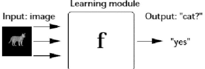
In computer vision the way it recognizes what objects are presented in a certain image is not a linear process, there are multiple techniques, however, the generic system may be represented as shown in Figure 1. (Riesenhuber & Poggio, 2000)

Figure 1 Object recognition system

In the previous figure, we have the basic architecture of an object recognition system. Essentially, the learning module is trained with a set of examples, corresponding to images previously labeled and can be described as a binary classifier. Based on an input image it retrieves as an output “yes” or “no”, for either the respective class of the object, like cat or dog or for the individual identity where the image belongs, for example, a face. (Riesenhuber & Poggio, 2000)

On top of an object recognition system, a slightly more detailed architecture was proposed, with more detailed components as shown in Figure 2. (Jain et al., 1995)

(13)

The Modelbase, also called Model database, contains all the known models in the system. The information inside depends essentially on the method used for the recognition and it goes from qualitative or functional description to precise geometric information, being this consider features of the object, with size, color or shape some of the common ones, allowing to describe and recognize the objects when compared to others. This component is organized with an indexing scheme of the features to help in the elimination of not desired object candidates from possible consideration during the hypothesis formation stage. (Jain et al., 1995)

The feature detector component applies a set of techniques in images to identify locations of features that help in the formation of the object hypothesis. The detected features vary on the different types of objects to be recognized and the organization of modelbase. With the features detected in the input image, it enters the hypothesis formation where it is assigned probabilities to objects presented in the image base on the recognition of certain features letting the system reducing the search space inside it. The verification of the hypothesis will use the models of the objects presented in the modelbase and then refine the probabilities of certain objects be in the image ending with the system selecting the objects with the highest probability. (Jain et al., 1995)

2.1.2 Object recognition techniques

Motivated by the challenges and the relevance of object recognition subject, over the last decade's multiple different techniques of object recognition were developed. These techniques are in symbiosis with the systems mentioned on the previous point being presented essentially on the learning module phase of the system.

Appearance-based

The object recognition using appearance-based techniques have been proposed to generalize the recognition systems being currently one of the most successful approaches to handling with 3D arbitrary objects when there is a disorder or partial obstruction of the object. (Selinger & Nelson, 2015)

(14)

Appearance is the only attribute to be used for this kind of techniques and normally is captured by different two-dimensional views of the object where it is possible to obtain two distinct types of features, global and local.

Local features are in small regions or single points of an image describing a portion of information about the image in that specific local. Essentially local features could be information about the color, gradient or even gray value of a certain pixel. (Latharani et al., 2011)

In distinction, global features have the goal to describe the entire image, all pixels in the image are considered and it varies from a simple mean value computation to shape or texture descriptors. (Lisin, Mattar, Blaschko, Learned-Miller, & Benfield, 2005)

Model based

This technique, that has as one of the main characteristics the division between the preprocessing and recognition stage, reducing the complexity of the algorithm, uses the model of an object to make some geometric transformations that map the model into a sensor coordinate system. With these, geometric algorithms draw results from computational geometry to detect the object. (Latharani et al., 2011)

Template-based

The template matching technique it is conceptually a simple process. Fundamentally, it tries to find a location of an object, based on its template, on an image by the match of the template. (Aljarrah & Ghorab, 2012)

For matching the template with the object in the input image, multiple geometrical parameters iterations, like rotation and scale, are performed to finding the required object.

Region based

This technique starts by transforming the original image, that comes as an input, into a directed graph, which is built based on various defined rules. The characteristics of the graph represent the global shape information of the object in the input image and are extracted while the graph is being constructed. (Latharani et al., 2011)

(15)

2.2 Deep Learning

The increase of machine-learning applications that are being used, for example, to object recognition in images and taking in concern the limitations of conventional machine-learning techniques in their capacity of processing natural data, in its raw format, leads to the use of advanced techniques of representation-learning called Deep Learning improving significantly areas of study such as speech recognition, object detection or even visual object recognition. (Yann LeCun et al., 2015)

This subdivision of machine learning comprises methods with several levels of representation of data that are obtained by composing modules where each one transforms the representation at one level into multiple levels of abstraction. With this information, it is possible to extract the set of features that characterize the combination of color, texture, and shape of an input image. (Yann LeCun et al., 2015)

2.2.1 Convolutional Neural Networks Individual Concepts

Convolution Neural Networks (CNNs) or also called ConvNets are not a novelty concept; in fact, studies around the late 1980s and 1990s about using neural networks to recognize handwritten zip codes or document recognition are well-known successful case studies of this concept being used in the early days. (Y. LeCun et al., 1989),(Yann LeCun, Bottou, Bengio, & Haffner, 1998)

The main characteristic and advantage of CNNs over standard neural networks is that they do not treat, from the input image, the pixels that are distance from each other in the same way as those which are close, taking essentially into account the local spatial structure of the image. Additionally, ConvNets architecture is well adapted to classification problems letting a faster training and consequently the creation of deeper networks with several layers being these days in multiple algorithms of object recognition. (Gomez, Cortes, & Noguer, 2015)

ConvNets, as standard neural networks have multiple sequential layers in a path that one-layer outputs are the inputs for the next one. Considering what was mentioned, many of neural networks concepts are used on CNNs, like gradient descent or backpropagation, however, due to the dimensionality issue, since CNNs allows to train deeper, with even

(16)

more layers, to avoid it, the concept of local receptive fields, pooling and shared weights and biases were introduced. (Gomez et al., 2015)

Local Receptive Fields

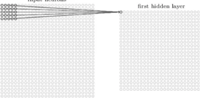
When comparing CNNs with common neural networks, one of the most distinctive characteristics of the ConvNets is the use of local receptive fields where convolutional layers input pixels will be connected to a layer of hidden neurons. This, against traditional neural networks, won’t connect every input pixel to every hidden neuron. In its place, convolutional layers will only connect to a small, localized region of the input image. (Nielsen, 2017)

The Figure 3 shows for 28x28 pixels (neurons) with 5x5 window corresponded to the local receptive field for the hidden neuron.

Figure 3 Local receptive fields

Based on the previous image, if we slide the local receptive field across the input image, and bear in mind that for each local receptive field there’s a hidden neuron, we will have a hidden layer of 24x24 neurons.

Figure 4 illustrates what is being stated, with the local receptive field window on the top-left of the corner of the input image.

(17)

Pooling

Another characteristic that distinguishes CNNs from the standard neural networks is the existence of pooling layers that achieves to simplify the information that arrives from the convolutional layers by reducing it. (Gomez et al., 2015)

Shared Weights and Biases

The last main difference of CNNs in comparison to standard neural networks is the use of unique shared weights and bias (or also called filter) for each hidden neuron on CNNs. This means that all neurons in a given convolutional layer will have the same response to the same feature from the previous layer, that can be for example a vertical edge. Essentially this is done due to the high probability of the learned feature to be useful in other parts of the image. In other words, the main consequence of sharing these bias is that the feature can be detected no matter where is in the image by getting the translation invariance property presented on CNNs. (Gomez et al., 2015)

2.2.2 Convolutional Neural Networks Basic Structure

According to one of the pioneers CNNs architecture, LetNet-5, proposed by Yann LeCun (1998), the CNN basic architecture must have the convolutional layer, pooling layer, and fully connected layers.

In overall, this architecture was the basis of another and more recent CNN architectures keeping, despite the improvements and modifications, the core concepts intact.

The Convolutional Layer

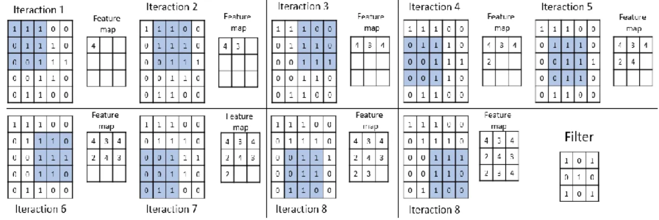
The idea of a convolution when talking of CNNs is to extract the features from an image preserving the spatial connection from the pixels and the learned features inside the image with the use of small equally-sized tiles.

The learned features are a consequence of a mathematical operation between each element from the input image and the filter matrix. In other words, the filter or also known as feature detector slides through all elements of the image and is multiplied by each one producing the sum of multiplication outputs a single matrix named Feature Map.

As stated Filters acts like a feature detector from the image and aren’t more than a matrix or matrices of pixels with depth - number of filters to use - and size parametrizable,

(18)

however depth together with the stride - number of pixels by which the filter matrix slides the input matrix - will control the size of the Feature Map matrix. (Andrew Gibiansky, 2015)

The next Figure shows a convolution of a 5x5 image with a 3x3 filter matrix and stride of 1.

Figure 5 Example of a convolution

Additionally, an operation called ReLU (Rectified Linear Unit) is usually used. ReLU is an activation function that adds non-linearity into the CNNs allowing it to learn nonlinear models. It is an operation on top of each pixel that replaces all negative pixels inside the feature map per zero. This rectifier technique is mostly used when compared with Hyperbolic Tangent or Sigmoid Functions since ReLU improves significantly the performance of CNNs for object recognition. (Gomez et al., 2015)

The Pooling Layer

As mentioned previously, one of the ConvNets distinctive concepts is pooling. The idea of the pooling step or spatial pooling is to reduce the dimensionality of each feature map, eliminating noisy and redundant convolutions, and computation network yet retaining most of the important information.

There are multiple pooling types, like, Max, Sum or Average, however the most common and preferred one is max-pooling. In max-pooling it is defined a spatial neighborhood and gets the max unit from the feature map based on that filter dimension that can be, for example, a 2x2 window. (Andrew Gibiansky, 2015)

(19)

Figure 6 shows an example of max-pooling operation, with a 2x2 window and stride of 2 taking the maximum of each region reducing the dimensionality of the Feature Map.

Figure 6 Example of max-pooling

The Fully Connected Layer

Being one of the latest layers of a ConvNet, coming right before the output layer, the Fully Connected layer works like a regular Neural Network at the end of the convolutional and polling layers where every neuron from the layer before the fully connected layer is connected to every neuron on the fully connected one.

The Fully Connected Layer purposes to use the output features from the previous layer (that can be a convolutional or a pooling layer) and classify the image based on the training dataset. (Wan et al., 2014)

2.3 Fast R-CNN for Object Recognition and Detection

Object recognition in images is one of the most directs uses of CNNs. As mentioned, recognize an object in an image has attached many challenges due to the variations that each object or the specific image could have like the illumination or viewpoint.

Early methodologies used sliding window and multiscale techniques with CNNs-extracted features and final classifiers, however, latest studies showed that training a CNN architecture that covers recognition and detection of the objects in an integrated approach are also a possibility with the introduction of new algorithms that learn to predict the creation of bounding boxes. (Sermanet et al., 2013)

Supporting what was mentioned is the work of Girshick (2015) using Fast Region-based Convolution Network (Fast R-CNN) proposing a fast and clean framework for object detection. This work was built on top of previous works that introduced the

(20)

Region-based Convolution Network (R-CNN) - Girshick, Donahue, Darrell, Malik, & Berkeley (2012) – and SPPnet – He, Zhang, Ren, & Sun (2015b) – however with multiple novelties that improved the training and testing velocity as well as the detection accuracy of the entire model. (Girshick, 2015)

Fast R-CNN enables an end-to-end detector combining all models into a single network. In other words, the Fast R-CNN framework trains a CNN, a classifier and a bounding box regressor in a unique model when previously, for example on R-CNN, we had a different model to extract features from the input image by using a CNN, to classify with an SVM and other for predict the bounding boxes. (Girshick, 2015)

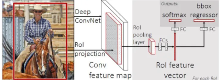
The Fast R-CNN architecture has some particularities starting in the input requirements taking, as usual on a ConvNet, an image and respective object annotations but in addition a set of object proposals representing the regions of interest (RoIs) of the images that will be used during the RoI pooling layer.

Primarily the network processes the entire image with multiple convolutional and pooling layers producing a convolutional feature map. This first operation is one of the gains, in terms of velocity, that Fast R-CNN achieves when compared with R-CNN since instead of running a CNN for each region of interest, it runs a single CNN for the entire image producing at the end the mentioned feature map. (Girshick, 2015)

Ended the first stage, the second part of the framework begins, where for each object proposal a RoI pooling layer, using max pooling, gets a small fixed size vector from the feature map and then mapped to a feature vector by a sequence of fully connected layers that finally splits into two output vectors per RoI: one for the classifier (usually softmax) to estimates the probability of each object class, and other with the bounding box regressor that outputs the coordinates for each object class. (Girshick, 2015)

In Figure 7, we are able to see the Fast R-CNN architecture based on what was explained before.

(21)

2.4 Related Work

In the most recent years, the use of CNNs has grown exponentially due to the multiple successful applications on solving extremely complex computer vision problems bringing that multiple advances in this area were being accomplished. However, some other successful works were made without the use of CNNs.

In this topic, it is intended to describe two different studies where object recognition and detection was applied based on two different approaches. The first one (Krizhevsky, Sutskever, & Hinton, 2012) with the use of CNNs and applying object recognition to the classification of generic images from ImageNet database. The second study (Jing et al., 2015) the main goal wasn’t the application of object recognition but yes visual search, leading to the necessity of previously using object recognition and location techniques as a consequence, using implementation of cascading deformable part-based models for the task.

2.4.1 Image Classification with Deep CNNs

The main goal of this article (Krizhevsky et al., 2012) was to train a large deep convolutional neural network to classify images from ImageNet, a dataset with over 15 million labeled images that belong to approximately 22000 different categories, into 1000 different classes for the LSVRC-2010 contest.

In order to achieve the objective, it was proposed an architecture with five convolutional layers and three fully connected ones. The output of the last fully connected layer produces close to 1000 class labels. Essentially the architecture focus on the delineation of responsibilities between two GPUs (Graphics processing unit) where one runs the top layers part and the second the bottom ones giving to only certain layers from each GPU the responsibility for the communication between the GPUs. Considering the mentioned architecture was possible to achieve an error rate around 17 and 37 percent, which according to the authors was the best until that date. (Krizhevsky et al., 2012)

More recent studies showed that the error rate inside this ImageNet contest is around 4.7%, goal accomplished by Microsoft research team. This achievement, based on previous experiments, even beat human beings, which achieve the 5.1% error rate. (He, Zhang, Ren, & Sun, 2015a)

(22)

2.4.2

Visual Search at Pinterest

This article (Jing et al., 2015) shows a prototype, developed by Pinterest and University of California, which aims to build, launch and maintain a visual search engine on top of the visual bookmarking tool, Pinterest.

As mentioned this article does not have has the main objective, object recognition, however, it is a consequence of using visual search engines. Due to the subject of the dissertation, this topic will only cover the object detection and localization chapter.

The architecture designed for the object detection has a two-step detection tactic that allows giving more importance to the free text titles on Pinterest images. Another important characteristic of the Pinterest is the possibility of pin an image, like giving a tag. With the information of the titles and pins aggregated it is possible to obtain a good information about the image is being analyzed. Given the textual metadata got, text-processing algorithms are applied on top of it, which allows to firstly predict what are the categories where the image belongs. This is a huge step in reducing computational costs since instead of running all object detection modules, it runs the needed ones that were predicted by the textual meta data information obtained. Another advantage of using this tactic is according to the authors, the reduction of false-positive rate. (Jing et al., 2015)

The optimization of the object detection method was made using cascading deformable part-based models that has as an output a bounding box for each object that was detected. Despite that, studies are being made on top of the performance and feasibility to use deep learning CNNs to detect the objects. (Jing et al., 2015)

(23)

Chapter 3 - System Implementation

This chapter starts by providing an overview of the development plan of the object detection system where explains the main steps to build it. After it is provided an explanation of the proposed architecture and an high-level description of all components. Then it is given a description of all technology stack involved with a resume of the hardware specifications where the system was developed and tested.

Subsequently it will be given an explanation of how were created the annotations for each image, that as stated, is one of the input requirements of Fast R-CNN, along with the input image itself and regions of interest.

Finally, it is given a detailed description of the entire components that composed the system. In this topic will be described the function of each component, how are related to each other and the main parameters available in the system that will affect the execution of the components.

3.1 Development Plan Overview

Due to a number of successful studies on using deep convolutional neural networks for object recognition and detection, being these presented as a good solution with high accuracy and efficiency on detect objects, this dissertation follow these references and keep the ConvNets as the approach for detecting objects in images.

As detailed on an earlier topic, Fast R-CNN became a really good solution not only because it is an end-to-end detector with good accuracy on detect objects but also it gave us the possibility of quickly train a new CNN enabling that new experiments could be done during the training and testing phase. Concerning this, and keeping in mind all requirements from Fast R-CNN, the proposed steps, in high-level view, to build the object recognition and detection system are:

1. Manual tagging the entire dataset with the regions of interest in each image; a. Split into training and testing data.

2. Train Fast R-CNN model;

(24)

3.2 System architecture

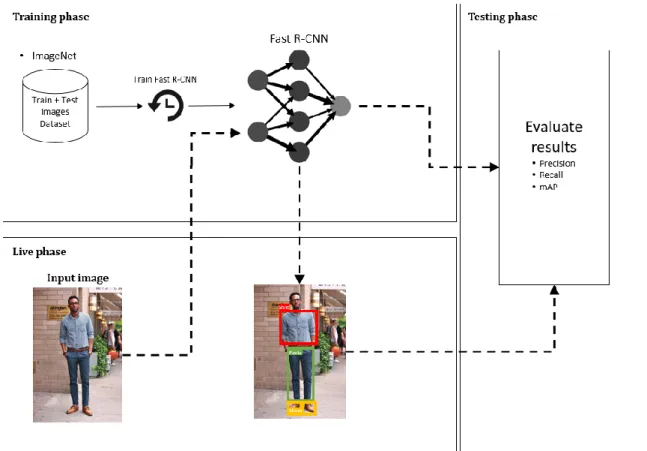
The main objective of the dissertation is by giving an image as an input to the system, it must be capable of detecting the fashion items available. In order to achieve this, first, we need to train a Fast R-CNN with a considerable amount of input images. These images will be extracted from ImageNet and then treated with the input requirements of the Fast R-CNN, already mentioned previously. After that will always occur an testing phase to evaluate the model in order to validate if it achieves the expected outputs.

With the Training phase accomplished, the second part starts, where given an input image to the pre-trained CNN, the output of the entire system must be the original image with the specific bounding boxes and respective description surrounding the fashion items inside. While live phase the idea is to interactively have a testing layer in order to test metrics like mean average precision of the entire system.

Figure 8 Proposed object detection system architecture illustrates the proposed system architecture with the respective distinctive components.

(25)

3.3 Technology Stack

First, it is important to mention that while the period of building this system, the tests and developments were made on a personal laptop, and not in a professional infrastructure with large RAM capacity or multiple GPUs to train the network. This means that we are always limited to the available hardware, which affects the evaluation and training delivery times. Despite that, no big blockers we have experienced in these phases being this one of the main reasons for choosing Fast R-CNN, namely, velocity on training the network.

Before any logic technology stack, it is important to know where everything runs, the hardware components, since as explained, it has a certain impact while developing and testing. Concerning this, the system hardware is composed by the following main components:

• Processor: Intel(R) Core(TM) i7-6700HQ 2.60GHz;

• Graphic card: NVIDIA GeForce GTX 1060 6GB GDDR5; • RAM: 16GB DDR4.

Focus now on logic technology stack, there are three main technologies to reinforce and were used to build the entire system:

• Python1_{was the programming language choose for orchestrating the whole}

system logic;

• CNTK2_{is an integrated deep-learning toolkit developed by Microsoft that}

supports Fast R-CNN;

• OpenCV3_{it is an open source computer vision library that was used in this}

project essentially for image manipulation.

1_{https://www.python.org/}

2 _{https://docs.microsoft.com/en-us/cognitive-toolkit/}_and

https://docs.microsoft.com/en-us/cognitive-toolkit/Object-Detection-using-Fast-R-CNN

(26)

Other Python libraries, were used to support operations like array manipulation, with NumPy4, or image processing, using PIL5, despite that multiple of these libraries are available on Anaconda6, a data science package manager available for python.

3.4 Image annotation

One of the biggest time-consuming tasks while training Fast R-CNN with a custom dataset, namely when we have thousands of images, is the annotation process since it is something that needs to be manually handled before the training phase.

Manual annotating an image, for this dissertation, was not only label the object presented in the image but link that label to specific coordinates (by drawing a bounding box that surrounds the object) that would be used later while training the model. Figure 9 shows an example of what was stated, being the blue box section that covers the shirt an example of a bounding box.

Figure 9 Example of a bounding box

In order to speed up the process, it was used the cross platform annotation tool for manual tagging image and videos, VOTT (Visual Object Tagging Tool)7. For this work, we will only focus on image tagging.

4_{http://www.numpy.org/}

5_{https://pypi.python.org/pypi/PIL} 6_{https://docs.continuum.io/}

(27)

The process of image manual tagging using VOTT, despite slow due to the big dataset, it is pretty straightforward, requiring just a few steps, namely:

1. After selecting to tag an image directory option, we need to load the image dataset folder;

2. With the dataset properly loaded, then it is required to configure the bounding box type (rectangle or square) and the respective labels/classes of the objects (shirts, pants, and glasses);

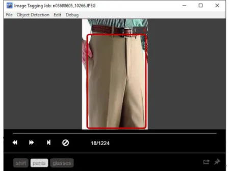
3. Finally, a new window appears for manual tagging each image available in the dataset by drawing a bounding box around the object and select the respective class, as shown in Figure 10.

Figure 10 VOTT example

Another advantage of using VOTT instead of other annotation script or even develop one, that would be an, even more, time-consuming, is that it provides already additional useful features, namely:

• After finished the manual tagging, it is possible to export the tags and bounding box coordinates in CNTK Fast R-CNN format;

• While exporting, VOTT creates the required Fast R-CNN folders (positive, negative and test) with the dataset properly divided, reserving a 20% of the tagged images, for the test set, which automatically supports our system without extended adjustments.

(28)

3.5 System components

The system components were developed with the support of Microsoft Cognitive Toolkit, or also known as CNTK, pre-compiled binaries. Concerning this, it became important to know a few better CNTK and its possibilities.

Developed by Microsoft Research team, CNTK is a unified deep-learning framework that establishes a good alternative to other deep-learning frameworks like Theano or TensorFlow allowing, amongst the others, structured implementation of the most popular deep neural networks architectures like CNNs, RNNs and recently Fast R-CNN.

According to multiple studies on top of CNTK, proved that it became one of the best deep-learning frameworks surpassing other frameworks in terms of speed, Shi, Wang, Xu, & Chu, (2016) or even accuracy Xiong et al., (2016).

Concerning this, and since CNTK is completely compatible with Python and Windows operating system, supporting yet Fast R-CNN implementation abstracting the user of the effort of building it manually, this framework became the understandable choice for developing the system.

Finally, it is important to mention that some of the source code system components available were built partially based on CNTK Fast R-CNN tutorial provided by Microsoft8 allowing to reduce the implementation time.

Each component has its own particular importance during the training and evaluation phase, however as it was implemented, there’s no direct communication between them which means that when a certain component execution ends, it produces one or more physical files (like input ROIs coordinated file or trained model) that will be required in the next component, however the next component must be manually launched by the user. The reason why it was developed like this was because each component is isolated from the others and most of the time it is executed without the need of executing the others (e.g. change the number of ROIs to extract from an image, only the first file, GenerateInputFile.py, needs to execute) avoiding redundant and time consuming steps.

(29)

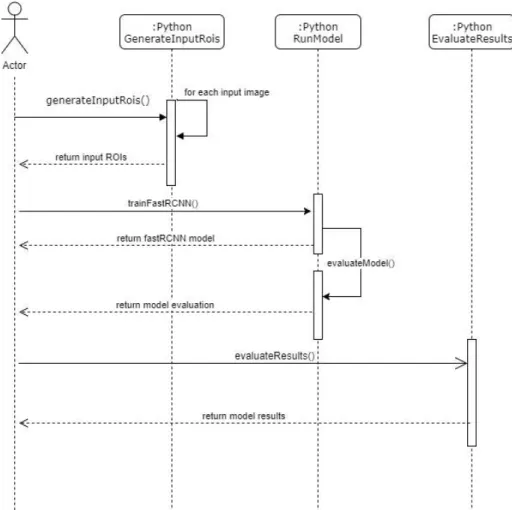
Figure 11 shows a sequence diagram of the system components presented during the evaluation and training phase. In the next points, will be discussed each component in detail.

Figure 11 Sequence diagram of system components

3.5.1 System folder tree

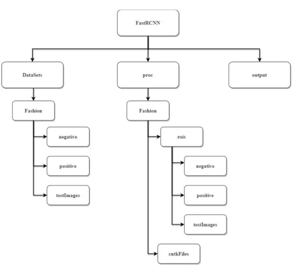
Due to the requirement of organizing the project system folder, it was created a folder structure, based on CNTK files organization, in order to store the dataset, output files and python scripts, organized in the respective folders. Concerning this, in Figure 12 is presented the folder tree of the developed system.

(30)

Figure 12 System folder tree

fastRCNN is the root folder, inside, amongst the other folders are presented the python files, namely, Parameters.py, GenerateInputROIs.py, RunModel.py and EvaluateOutput.py.

Inside DataSets folder are the input images for training and testing the model with the respective annotation files. These images are separated in three folders, depending on what will be used.

The proc folder is from where the final ROIs for each image will be written. The rois subdirectory as the previous point is also divided depending on if the ROIs belong to a

(31)

positive, negative or test image. The cntkFiles subdirectory contains the input files for images, the ROI coordinates and ROI labels – all in CNTK format9.

Finally, the output folder is where the trained model will be stored.

3.5.2 Parameters

During the implementation, some configurable parameters were used that helped built and optimize the system. With the parameters section available on Parameters.py file it was possible to have a single place of configurations without the need of further configurations on the other components.

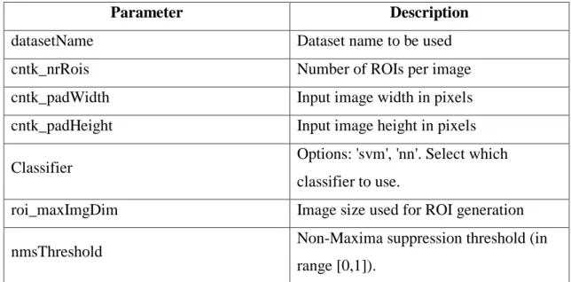
Table 1 System parameters show a resume of the main parameters available.

Parameter Description

datasetName Dataset name to be used

cntk_nrRois Number of ROIs per image

cntk_padWidth Input image width in pixels

cntk_padHeight Input image height in pixels

Classifier Options: 'svm', 'nn'. Select which

classifier to use.

roi_maxImgDim Image size used for ROI generation

nmsThreshold Non-Maxima suppression threshold (in

range [0,1]).

Table 1 System parameters

The datasetName parameter is where it is configured which data should be used. This is important essentially because if there is a need of having multiple configured datasets, we just need to change a single parameter to be reflected in the system.

The cntk_nrRois is a parameter that tells the system how many ROIs should be used for training and testing. This parameter is particularly important due to the impact that will have on system execution times since the lower the value, the quicker the system will be, however without expectation of good results.

9

(32)

The cntk_padWidth and cntk_padHeight parameters reflect the deep neural network input image size. These parameters are required because the Fast R-CNN model required that all images be with the same size converting each image for the specified size.

The Classifier parameter tells the system which classifier should be used. Consequently of the current Fast R-CNN implementation available on CNTK, currently it is only possible to use Support Vector Machine (‘svm’ option) or softmax (‘nn’ option) The roi_maxImgDim parameter tells the max image size used for ROI generation. The bigger the parameters, objects with higher dimensions are easily detected, however, this parameter should be carefully configured because we can’t increase it significantly with the consequence of affecting the detection of small objects.

The nmsThreshold tells the system the non-maxima suppression threshold that affects the combination of ROIs - the lower the value more ROIs will be combined.

3.5.3 Generate Input ROIs component

Regions of interest (ROI) can be defined as a set of samples within a dataset that is identified for a specific purpose. A common example is applied to images, being an ROI a portion of an image that it is intended to filter to perform operations on top of it. (Brinkmann, 2008)

The Generate Input ROIs component (GenerateInputROIs.py) logic is divided into three stages that will at the end generate ROIs candidates for each image. These ROIs are then converted into CNTK format and stored in rois and cntkFiles subdirectories, described already on System folder tree section, to be then executed in Fast R-CNN model.

The script starts by generating for each input image ROI candidates. This task is done recurring to selective search technique that produces, per image, a huge number of ROIs. Selective search is a method for discovering a considerable set of probable object locations in an image, disregarding the actual object class. It works by grouping the image pixels into segments, performing then hierarchical clustering to gather segments from the same object into regions of interest. (Uijlings, Van De Sande, Gevers, & Smeulders, 2012)

(33)

The main goal of ROIs generation is to find a minor group of ROIs that however cover tightly, as many as possible, the distinct objects presented in the image. The second stage came to help in that process since despite selective search works well on producing those ROI candidates, it produces also, multiple bigger, smaller and identical ROIs. With that, the task of the second stage is to discard those ROIs that will not be useful during the training and testing phase. Lastly, the third stage adds supplementary ROIs at different aspect ratio and scales that cover the image integrally.

Figure 13 shows an example of an image with respective ROI candidates after selective search, being the green and red rectangles the ROIs that were considered after second stage and the blue rectangles the ones that were excluded.

(34)

3.5.4 Train Fast R-CNN model component

This component will train a new Fast R-CNN model and generate the model output file and additional required files that will be used for future evaluations. As stated, CNTK provides an implementation which reduced the system implementation time. With this in mind, in order to train the model it is only required to properly configure the system configuration file (Parameters.py) with a special attention to classifier parameter that will affect the model execution and on predicting the ROI labels and scores or also named detection confidence.

An important subject related to the Fast R-CNN model training rests on the base model that is being used. Currently, for CNTK, the only available base model is AlexNet with some adaptions in order to follow the Fast R-CNN architecture.

AlexNet is a deep convolutional neural network developed by Krizhevsky et al., (2012) submitted to the ILSVRC challenge in 2012, winning the contest. Its basic architecture is similar to LetNet but bigger and deeper, having as a main difference than the previous architectures at the time, the use of multiple convolutional layers loaded on top of each other instead of a single convolutional layer followed by pooling layer.

CNTK Fast R-CNN implementation has as its basis on AlexNet deep neural network, however, in order to make it plausible for a Fast R-CNN architecture, an ROI pooling layer was introduced between the last convolutional layer and the first fully connected layer of the AlexNet base architecture.

One of the main differences between CNTK Fast R-CNN implementation and the original experiment by Girshick (2015) is the model architecture since, in CNTK implementation, there’s no bounding box regression layer, instead this model works by classifying proposal regions of each image, as belonging to one of a set of existent object classes, or as ‘background’ class. All images are treated by a sequence of convolutional layers and then, for each proposal region, convolutional features with spatial support conforming to that region are extracted and resized to a fixed dimension, before being passed through three fully-connected layers, the last of which yields a score for each object class and ‘background’. The class scores for each region are then loaded into a softmax classifier function, to produce a distribution over classes. (Henderson & Ferrari, 2017)

(35)

At the end of the training, it starts the first part of the evaluation stage, where for each image, the predicted ROIs and labels are stored in FastRCNN/proc/Fashion/cntkFiles subdirectory to be further used while evaluating the results, on the EvaluateResults component.

3.5.5 Evaluate Results component

Once ended the training stage and the predicted ROIs and labels properly stored in the respective subdirectory, the Evaluate Results component can be used. Essentially this component intends to parse the output files provided and compute the classifier accuracy by returning the model mean Average Precision for the testing set.

The model quality can be measured by using multiple different criteria’s such as recall, accuracy, precision, amongst the others, however, a usual metric is, for each object class, measure the system average precision, being the mean Average Precision (mAP) the average of average precision of all classes.

The idea of computing Average Precision is due to its value for evaluating a certain model in terms of classification and detection capacity. This metric combines recall and precision metrics, by computing for each class the precision/recall curve, being very sensitive to the ranking of retrieval results, since the lower ranking results have less impact than the results in the higher rank.

With this in mind, the computation of Average Precision can be described as a sum of precisions at every possible threshold value multiplied by the change in the recall:

∑ 𝑃(𝑘) ∆𝑟(𝑘)

𝑁

𝑘=1

Where,

• N is the images total number;

• 𝑃(𝑘) the precision at cutoff time of k images

(36)

In resume, if we had the following hypothetical results, shown in Table 2, in that exact order:

Retrieval cutoff Precision Recall ∆𝑟(𝑘)

Top 1 image 100% 20% 0.2 Top 2 images 100% 40% 0.2 Top 3 images 66% 40% 0 Top 4 images 75% 60% 0.2 Top 5 images 60% 60% 0 Top 6 images 66% 80% 0.2 Top 7 images 57% 80% 0 Top 8 images 50% 80% 0 Top 9 images 44% 80% 0 Top 10 images 50% 100% 0.2

Table 2 Precision/Recall example

The average precision metric would be:

𝐴𝑃 = (1 ∗ 0.2) + (1 ∗ 0.2) + (0.66 ∗ 0) + (0.75 ∗ 0.2) + (0.6 ∗ 0) + (0.66 ∗ 0.2) + (0.57 ∗ 0) + (0.5 ∗ 0) + (0.44 ∗ 0) + (0.5 ∗ 0.2) = 0.782

Finally, the results can be visualized, showing only the ROIs and respective classes that have a detection confidence above 0.5. In order to visualize the final results, it is applied Non-Maxima Suppression (NMS) technique that tries to identify which ROI best cover the object by selecting the one with the highest confidence, removing the other ROIs for the same class that overlaps the “best” ROI.

Figure 14 shows an example of a before and an after Non-maxima suppression application being possible to distinguish multiple predicted ROIs, with its detection confidence, that were deleted after running NMS leaving only one ROI for shirt class that represents the best-located ROI for the object.

(37)

(38)

(39)

Chapter 4 - Results Evaluation

In order to evaluate the system and its capabilities, it is important to measure it in two different perspectives namely, the duration that takes on training the model and the system performance on detecting and classifying an image set.

Concerning this, two different parameters will be varied while training/testing in order to measure its impact in the system. The first parameter is cntk_nrRois that theoretically affects system times and performance so it is expected to be one of the most critical parameters. The second is related to nmsThreshold that only affects the testing stage so only the system performance on detecting and classifying an image, however, due to its purpose already stated on Parameters section it is expected to have a few impact which becomes an interesting parameter to test.

The classifier that will be used for training and testing stages will be softmax. Currently, CNTK only supports softmax and SVM, however, these experiments will follow the Fast R-CNN paper, Girshick (2015), that used softmax and proved that for the Fast R-CNN algorithm, it worked better than SVM classifier.

All experiments will be on top of ImageNet custom dataset, already described on system implementation section. With that, the first point, based on the training set available, will test the impact of cntk_nrRois on model execution times, by measuring the time it takes to train a Fast R-CNN model by varying that parameter.

After, as specified, will be presented the results evaluation of the system in terms of its capability of detecting and classifying the images available in the testing set, being these results presented by using a precision/recall curve plot and average precision metric, per class. With that, variations of cntk_nrRois and nmsThreshold values will be performed to measure the impact on the mentioned metrics.

Finally, a cross results evaluation will be performed, aggregated to cntk_nrRois variations, to assess the real impact of change this parameter in terms of system performance.

(40)

4.1 Train and test data

For the respective object recognition and detection system, it was created a custom dataset with images extracted from ImageNet. In order to accomplish the dissertation objectives and due to a number of fashion items available from multiple distinct categories, it was chosen to select three diverse categories to detect: one for each body part, lower and upper body, and another related to fashion accessories.

For the lower body, it was selected generic pants. The idea is to detect pants, no matter the type (jeans, straight pants, etc). This thought is shared with the category fashion accessories where it is intended to detect glasses, no matter if are eyeglasses or sunglasses. For the upper body, there’s a distinction when compared with the other two categories, the idea is to detect specifically shirts. This means that we intend to detect shirts but not relatives, like sweatshirt or t-shirts.

Another custom set of data was extracted from ImageNet that concerns to negative images to be used during the network training, being the only dataset that doesn’t belong and doesn’t have the categories to be detected. This last dataset has multiple different categories going from, animals, flowers, cars, appliances and other random images.

Finally, the dataset was divided into 80% for the training set and 20% for the test set. This is supported by the need of having low variance while testing data and still have the amount of data required to have low variance in the training set too.

Table 3 shows the number of images available in the training dataset per its different categories and type.

Type Category # of Images

Positive Pants 981

Positive Shirts 1144

Positive Glasses 1040

Negative Appliances 153

Negative Other Fashion items 93

(41)

Negative Animals 64

Negative Flowers 43

Negative Others 84

Total 3677

Table 3 Train images per category

As it possible to see through the Table 1 analysis, the training data will have a total of 3677 distinct images belonging to around 86% (3165 images) to a positive set of images and 14% (512 images) to the negative set. Focus on positive training set, it was intended to have similar number of images between categories, being however, the shirts category the one with higher number, 1144 images (~31%), followed by glasses category with 1040 images (~28%) and last pants category with 981 images (~26%).

Focus now on the test dataset, Table 4 resumes the spare of images amongst the different categories. Note that, inside test dataset there is no negative images since this type of images are only to be used during the training period.

Category # of Images

Pants 208

Shirts 268

Glasses 220

Total 696

Table 4 Test images per category

In the test set, as it occurs on the training set for the positive categories, it is intended to have a similar number of images across categories. Concerning this and for a total of 696 images, we have around 30% (208 images) of pants, 39% of shirts (268 images) and 31% of glasses (220 images).

(42)

4.2 Model Training Time Analysis

One of the most interesting evaluations on top of object detection systems is the time it takes while training the model. This state is supported by the multiple analysis made on an diversified number of papers around this kind of systems, namely as an example He et al., (2015b) or Girshick et al., (2012), that had as a main goal the assessment of the improvement or lost in terms of speed that their solutions had, while compared to other algorithms or by varying parameters.

For this test, the focus will be on testing the model training duration by varying one specific parameter, namely cntk_nrRois, and evaluate its impact on training time. With this, Table 5 shows a resume of the obtainable results for three distinct cntk_nrRois possible values.

Test name cntk_nrRois Duration (in minutes)

Test200 200 31.55

Test2000 2000 187.9

Test4000 4000 358

Table 5 Model testing time per cntk_nrRois variation

In order to help the analysis, Figure 15 provides graphically the stated results.

Figure 15 Model testing time per cntk_nrRois variation 0 50 100 150 200 250 300 350 400

(43)

As it can be observed, the cntk_nrRois parameter has a huge impact in model training times increasing significantly the delivery of a trained model. In other words, if a given trained model that has cntk_nrRois value configured to 200 requires to be re-trained with 10x more number of ROIs, so 2000, to be extracted during selective search, this will have an increase of around 496% (156 minutes) in the whole system training time or close to 1035% (~326 minutes) if instead we choose to grow the value 20x more, 4000 ROIs. This state is also visible if we want to increase the number of ROIs from 2000 to 4000 since the model will take around 90% more time (~170 minutes) to execute.

The increase of time from a theoretical perspective is plausible since more ROIs are extracted on selective search more ROIs will be pooled into each feature map and consequently more time for classification and prediction steps. Despite that, it became even more important and interesting to analyze the impact of cntk_nrRois variation on system performance on detecting and classifying the objects.

4.3 Recognition and Detection Results Analysis

The performance of an object recognition and detection system engine on classifying and locate objects in images is possibly the most important analysis that it is likely to do on top of this kind of systems since it will give an overall notion on if it is doing what it intends to do or not.

Some metrics can be used to measure these systems like precision, recall, area under curve, and others. With this, the idea to accomplish these tests is to combine these metrics through a precision/recall curve and area under curve, also known as average precision, and analyze the obtained results.

Another important topic is due to the parameters that will be varied while testing. As stated these parameters are cntk_nrRois and nmsThreshold and the values will be varied in order to measure the impact in performance. The first parameter cntk_nrRois value will be a consequence of the trained models that were done for training time analysis, so currently we have three different Fast R-CNN models where one was trained with cntk_nrRois = 200 another 2000 and the last 4000.

(44)

Regarding nmsThreshold, the tests will be made by varying it in a set of values of [0.01; 0.3; 0.5]. The idea is for each trained module we vary the non-maxima suppression threshold parameter and evaluate its impact.

Table 6 Parameters values per test resume the values of all parameters in each test that will be performed.

Test name cntk_nrRois nmsThreshold

Test200_001 200 0.01 Test200_03 200 0.3 Test200_05 200 0.5 Test2000_001 2000 0.01 Test2000_03 2000 0.3 Test2000_05 2000 0.5 Test4000_001 4000 0.01 Test4000_03 4000 0.3 Test4000_05 4000 0.5

(45)

4.3.1 Test200_001

The obtained results for Test200_001 with cntk_nrRois = 200 and nmsThreshold =

0.01 can be observed in Figure 16 Precision-Recall curve per class for Test200_001 with

a Precision-Recall curve per class being then resumed in Table 7 by showing the average precision for each class and mean average precision, in percentage, for the respective test.

Figure 16 Precision-Recall curve per class for Test200_001

shirt pants glasses mAP

0.7699 0.6349 0.4185 0.6078

Table 7 Average precision for Test200_001

Analyzing the Precision-Recall curve it is possible to conclude that for low recall values, pants is the class where our model achieves better precision, however after ~50% recall it has a significant decrease in precision which turns shirt as the class with overall best precision, having yet a significant precision decrease close to 80% recall. This fact is supported by the average precision computation that shows shirts as the class with better AP, close to 77%, superior to pants with AP of ~63% and glasses, achieving an AP of ~61%. With this, overall the model with these configurations achieved a mean average precision (mAP) of ~61%.

(46)

4.3.2 Test200_03

The obtained results for Test200_03 with cntk_nrRois = 200 and nmsThreshold = 0.3 can be observed in Figure 17 Precision-Recall curve per class for Test200_03 with a Precision-Recall curve per class being then resumed in Table 8 by showing the average precision for each class and mean average precision, in percentage, for the respective test.

0.7797 0.6488 0.4322 0.6202

As it possible to see on Precision-Recall curve, in general, shirt class is where our model has better overall precision having, however, a huge decrease after 80% recall. The average precision of shirts is ~78%, bigger than pants, that has ~65% and glasses with ~43% average precision as it possible to visualize on Table 8, corroborating what was stated. The model mean average precision, for these specific configurations is ~62% being until this point, the best mAP achieved.

(47)

4.3.3 Test200_05

The obtained results for Test200_05 with cntk_nrRois = 200 and nmsThreshold = 0.5 can be observed in Figure 18 Precision-Recall curve per class for Test200_05 with a Precision-Recall curve per class being then resumed in Table 9 by showing the average precision for each class and mean average precision, in percentage, for the respective test.

0.7379 0.6082 0.4055 0.5839

By visualizing the Precision-Recall curve we can conclude that shirt class is, when compared with the previous points, once again, the class with overall best precision with around 74%. Despite that these configurations, for cntk_nrRois = 200 proved to be, until now, the poorest since all average precisions decreased and consequently the mAP, being ~58% inferior than the previous with ~61% for Test200_001 and ~62% for Test200_03.

(48)

4.3.4 Test2000_001

The obtained results for Test2000_001 with cntk_nrRois = 2000 and nmsThreshold

= 0.01 can be observed in Figure 19 Precision-Recall curve per class for Test2000_001

with a Precision-Recall curve per class being then resumed in Table 10 by showing the average precision for each class and mean average precision, in percentage, for the respective test.

0.7700 0.6061 0.5427 0.6396

Looking for Figure 19 that shows the Precision-Recall curve per class for these specific configurations it is possible to observe that our model continues to have a better precision on shirt class, being this confirmed by the computation of average precision, resumed on Table 10, higher than pants with ~61% average precision and ~54% average precision for glasses. It became interesting to highlight the growth of average precision of glasses class when compared with the previous tests, increasing more than 11% affecting positively the mAP measure achieving the best result until now with ~64%.

(49)

4.3.5 Test2000_03

The obtained results for Test2000_03 with cntk_nrRois = 2000 and nmsThreshold =

0.3 can be observed in Figure 20 Precision-Recall curve per class for Test2000_03 with

a Precision-Recall curve per class being then resumed in Table 11 by showing the average precision for each class and mean average precision, in percentage, for the respective test.

0.7738 0.6274 0.5579 0.6530

Observing the Precision-Recall curve of Figure 20 it is possible to visualize that pants and glasses tend to have similar precisions for levels of recall between 65 and 75 percent. Despite that, these similar results happen only when the precision value is decreasing, however for the low level of recalls this state isn’t valid affecting the difference of values of model average precision for both classes being pants higher with ~63% than glasses with ~56%. Shirt class continues to be where our model achieves the best average precision with ~77% being the mAP as ~65%, the best mean average precision achieved until now.