GRADUATE PROGRAM IN ELECTRICAL AND COMPUTER
ENGINEERING
HUGO ALBERTO PERLIN
A CONTRIBUTION TO SEMANTIC DESCRIPTION OF IMAGES
AND VIDEOS: AN APPLICATION OF SOFT BIOMETRICS
DOCTORAL THESIS
A CONTRIBUTION TO SEMANTIC DESCRIPTION OF IMAGES
AND VIDEOS: AN APPLICATION OF SOFT BIOMETRICS
Doctoral Thesis presented to the Graduate Program in Electrical and Computer Engineering of the Federal University of Technology - Paran´a as partial fulfillment of the requirements for the title of “Doctor of Science (D.Sc.)” – Concentration Area: Computer Engineering.
Thesis Advisor: Heitor Silv´erio Lopes
Perlin, Hugo Alberto
P451c A contribution to semantic description of images and vídeos : 2015 an application of soft biometrics / Hugo Alberto Perlin.-- 2015.
109 f. : il. ; 30 cm.
Texto em inglês, com resumo em português
Tese (Doutorado) - Universidade Tecnológica Federal do Paraná. Programa de Pós-graduação em Engenharia Elétrica e Informática Industrial, Curitiba, 2015
Bibliografia: p. 103-109
1. Visão por computador. 2. Aprendizado do computador. 3. Processamento de imagens. 4. Interpretação de imagens. 5. Linguagem de programação (Computadores) - Semântica. 6. Engenharia elétrica - Dissertações. I. Lopes, Heitor Silvério. II. Universidade Tecnológica Federal do Paraná - Programa de Pós-Graduação em Engenharia Elétrica e Informática Industrial. III. Título.
Câmpus Curitiba
Programa de Pós-Graduação em Engenharia Elétrica e Informática Industrial
Título da Tese Nº. 129
A Contribution to Semantic Description of Images
and Videos: an Application of Soft Biometrics
por
Hugo Alberto Perlin
Orientador: Prof. Dr. Heitor Silvério Lopes
Coorientador: Prof. Dr.
Esta tese foi apresentada como requisito parcial à obtenção do grau de DOUTOR
EM CIÊNCIAS – Área de Concentração: Engenharia de Computação, pelo
Programa de Pós-Graduação em Engenharia Elétrica e Informática Industrial –
CPGEI – da Universidade Tecnológica Federal do Paraná – UTFPR, às 14:00h do
dia 08 de dezembro de 2015. O trabalho foi aprovado pela Banca Examinadora,
composta pelos doutores:
_____________________________________ Prof. Dr. Heitor Silvério Lopes
(Presidente – UTFPR)
___________________________________ Prof. Dr. Alessandro Lameiras Koerich (ÉCOLE DE TECHNOLOGIE SUPÉRIEURE)
__________________________________ Prof. Dr. Alceu de Souza Britto Jr.
(PUC-PR)
___________________________________ Prof. Dr. Chidambaram Chidambaram
(UDESC – São Bento do Sul)
__________________________________ Profª. Drª. Lúcia Valéria Ramos de Arruda
(UTFPR)
__________________________________ Prof. Dr. Hugo Vieira Neto
(UTFPR)
Visto da Coordenação:
__________________________________ Prof. Dr. Emilio Carlos Gomes Wille
During the doctoral program, we are constantly put to test. Several times there are
many more questions and doubts rather than clarity on how to proceed. But certainly, the
people who were constantly at my side, near or far, were responsible for getting me to the end.
To them, I am very grateful.
First, my wife Michele and my son Bento, by love, support, patience, warmth and
comfort. Several times my presence was far, but even so, they continued to support and
encourage me. This work was possible because of them.
My parents Antonio and Marinez, and my brother Jo˜ao, who taught me the true values
of life and built the foundation for my growth.
I would like to thank Professor Heitor Silv´erio Lopes for the confidence, patience and
persistence. From a mentoring relationship, a good friendship raised. Thank you for the lessons
and the kilometers shared.
To friends and companions of Bioinfo laboratory, Cesar Vargas Benitez, Ademir
Gabardo, Chidambaram Chidambaram, Jonas Fries Krause, Rodrigo Silva, Manass´es Ribeiro,
Leandro Hattori, Andr´e Barros, Gl´aucio Porcides and Fernando Carvalho de Souza, for good
conversations and laughter, the huge amount of coffee, the discussion of ideas and suggestions.
Much of this work has a good piece of your contribution.
The Federal Institute of Paran´a, for their support in allowing part of the PhD to be
carried out with exclusive dedication.
In short, everyone who in one way or another showed their appreciation for me. Thank
PERLIN, HUGO ALBERTO. A CONTRIBUTION TO SEMANTIC DESCRIPTION OF IMAGES AND VIDEOS: AN APPLICATION OF SOFT BIOMETRICS. 110 f. Doctoral Thesis – Graduate Program in Electrical and Computer Engineering, Federal University of Technology - Paran´a. Curitiba, 2015.
Humans have a high ability to extract information from visual data acquired by sight. Trough a learning process, which starts at birth and continues throughout life, image interpretation happens almost instinctively. At a glance, one can easily describe a scene with reasonable accuracy, naming its main components. Usually, this is done by extracting low-level features such as edges, shapes and textures, and associating them to high level meanings. In this way, a semantic description of the scene is done. An example of this is, the human ability to recognize and describe other people’s physical and behavioural characteristics, or biometrics. Soft-biometrics also represents inherent characteristics of human body and behaviour, but they do not allow unique person identification. The computer vision area aims to develop methods able to performing visual interpretation with human similar performance. This thesis aims to propose computer vision methods which allows high level information extraction from images and videos in the form of soft biometrics. This problem is approached in two ways, trough unsupervised and supervised learning methods. The first way, is intended to group images via an automatic feature extraction learning, using both convolution techniques, evolutionary computing and clustering. In the 1st approach the images used contain faces and people. The second approach employs convolutional neural networks, which have the ability to operate directly on raw images, learning both feature extraction and classification processes. Here, images are classified according to gender and clothes, divided into upper and lower parts of the human body. The first approach, when tested with different image datasets obtained an accuracy of approximately 80% for faces and non-faces and 70% for people and non-people. The second approach, which was tested using images and videos, have obtained an accuracy of about 70% for gender, 80% for the upper clothes and 90% for lower clothes. The results of these case studies show that the proposed methods are promising, allowing the realization of automatic annotation of high level image information. This opens possibilities for development of applications in diverse areas such as content-based image and video search and automatic video surveillance, reducing human effort in the task of manual annotation and monitoring.
PERLIN, HUGO ALBERTO. UMA CONTRIBUIC¸ ˜AO PARA DESCRIC¸ ˜AO SEM ˆANTICA DE IMAGENS E V´IDEOS: UMA APLICAC¸ ˜AO DE BIOMETRIAS FRACAS. 110 f. Tese de doutorado – Programa de P´os-graduac¸˜ao em Engenharia El´etrica e Inform´atica Industrial, Universidade Tecnol´ogica Federal do Paran´a. Curitiba, 2015.
Os seres humanos possuem uma alta capacidade de extrair informac¸˜oes de dados visuais, adquiridos por meio da vis˜ao. Atrav´es de um processo de aprendizado, que se inicia ao nascer e continua ao longo da vida, a interpretac¸˜ao de imagens passa a ser feita de maneira quase instintiva. Em um relance, uma pessoa consegue facilmente descrever com certa precis˜ao os componentes principais que comp˜oem uma determinada cena. De maneira geral, isto ´e feito extraindo-se caracter´ısticas de baixo n´ıvel, como arestas, texturas e formas, e associando-as com significados de alto n´ıvel. Ou seja, realiza-se uma descric¸˜ao semˆantica da cena. Um exemplo disto ´e a capacidade de reconhecer pessoas e descrever suas caracter´ısticas f´ısicas e comportamentais. A ´area de vis˜ao computacional tem como principal objetivo desenvolver m´etodos capazes de realizar uma interpretac¸˜ao visual com desempenho similar aos humanos. Estes m´etodos englobam conhecimentos de aprendizado de m´aquina e processamento de imagens. Esta tese tem como objetivo propor m´etodos de vis˜ao computacional que permitam a extrac¸˜ao de informac¸˜oes de alto n´ıvel na forma de biometrias fracas. Estas biometrias representam caracter´ısticas inerentes ao corpo e ao comportamento humano. Por´em, n˜ao permitem a identificac¸˜ao un´ıvoca de uma pessoa. Para tanto, este problema foi abordado de duas formas, utilizando aprendizado n˜ao-supervisionado e supervisionado. A primeira busca agrupar as imagens atrav´es de um processo de aprendizado autom´atico de extrac¸˜ao de caracter´ısticas, empregando t´ecnicas de convoluc¸˜aos, computac¸˜ao evolucion´aria e agrupamento. Nesta abordagem as imagens utilizadas contˆem faces e pessoas. A segunda abordagem emprega redes neurais convolucionais, que possuem a capacidade de operar diretamente sobre imagens cruas, aprendendo tanto o processo de extrac¸˜ao de caracter´ısticas quanto a classificac¸˜ao. Aqui as imagens s˜ao classificadas de acordo com gˆenero e roupas, divididas em parte superior e inferior do corpo humano. A primeira abordagem, quando testada com diferentes bancos de imagens, obteve uma acur´acia de aproximadamente 80% para faces e n˜ao-faces e 70% para pessoas e n˜ao-pessoas. A segunda, testada utilizando imagens e v´ıdeos, obteve uma acur´acia de cerca de 70% para gˆenero, 80% para roupas da parte superior e 90% para a parte inferior. Os resultados destes estudos de casos, mostram que os m´etodos propostos s˜ao promissores, permitindo a realizac¸˜ao de anotac¸˜ao autom´atica de informac¸˜oes de alto n´ıvel. Isto abre possibilidades para o desenvolvimento de aplicac¸˜oes em diversas ´areas, como busca de imagens e v´ıdeos baseada em conte´udo e seguranc¸a por v´ıdeo, reduzindo o esforc¸o humano nas tarefas de anotac¸˜ao manual e monitoramento.
–
FIGURE 1 Steps of a traditional image classification process. . . 23 –
FIGURE 2 Example of describing an image of a person using soft biometric attributes. 28 –
FIGURE 3 Example of a neuron, showing the inputs, the weighted sum, the activation function and the output. . . 29 –
FIGURE 4 Example of an multilayer network. . . 30 –
FIGURE 5 An example of a CNN architecture. The dashed rectangle denotes the feature extractor layers. The continuous rectangle denotes the classifier layers. The (I) layer represents the raw input image. The (C) layers represent convolution operations. The (S) denotes sub-sampling operations. The linear layers are represented by (L), and (O) represents the output layer. . . 32 –
FIGURE 6 LeNet-5 network architecture, which was proposed to classify handwritten digits. . . 34 –
FIGURE 7 CNN architecture proposed by (KRIZHEVSKY et al., 2012) as solution to ILSVRC2010. . . 36 –
FIGURE 8 Representation of how dropout works. . . 36 –
FIGURE 9 A hypothetical good clustering result, where similar objects are close together and there is a distance between the groups. . . 42 –
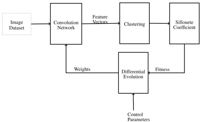
FIGURE 10 Block diagram representing the main steps for the proposed unsupervised feature learning framework. . . 51 –
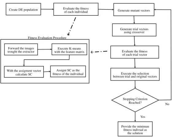
FIGURE 11 Flowchart showing the proposed method. Dashed lines indicates a sub-process. . . 54 –
FIGURE 12 Hand-designed feature extraction and classification process. . . 59 –
FIGURE 13 Example of mean filtering of an output. The blue line is the original signal, and other lines represent the signal filtered by different window sizes. The solid black line is the target, and the dashed line represents a threshold. . . 64 –
FIGURE 14 Samples from the Faces Dataset. The three first rows show examples for the Face class, while the last three for the Background class. . . 67 –
FIGURE 15 Samples from the Pedestrian Dataset. The three first rows show examples for the Person class, while the last three for the Background class. . . 68 –
FIGURE 16 Examples of frames used as evaluation dataset. Annotation bounding boxes were used to extract patches with people from each frame. . . 70 –
FIGURE 17 ROC graph comparing the performance of the two different models trained using the Face dataset. . . 72 –
FIGURE 18 ROC graph comparing the performance of the two different models trained using the Pedestrian dataset. . . 72 –
FIGURE 19 ROC curves and the area under the curve values for each combination of feature extractors and SVM classifiers for Faces dataset. . . 74 –
FIGURE 20 ROC curves and the area under the curve values for each combination of feature extractors and SVM classifiers for Pedestrian dataset. . . 75 –
–
FIGURE 23 Comparison of hand-designed classifiers according to ranking methods and number of top features, for the Lower Clothes attribute. . . 79 –
FIGURE 24 Accuracy curve during OM #1 CNN training for the Gender Clothes attribute. . . 80 –
FIGURE 25 Accuracy curve during OM #1 CNN training for the Upper Clothes attribute. . . 81 –
FIGURE 26 Accuracy curve during OM #1 CNN training for the Lower Clothes attribute. . . 82 –
FIGURE 27 Box-plot chart showing the distribution of the three methods for the gender attribute. . . 83 –
FIGURE 28 Box-plot chart showing the distribution of the three methods for the upper clothes attribute. . . 84 –
FIGURE 29 Box-plot chart showing the distribution of the three methods for the lower clothes attribute. . . 85 –
FIGURE 30 The top-10 OM #1 CNN results for each class. First and Second Rows:
samples classified as Long and Short for Upper Clothes. Third and Fourth Rows: samples classified as Long and Short for Lower Clothes. Fifth and Sixth Rows:samples classified as Female and Male for Gender. . . 86 –
FIGURE 31 The top-10 OM #1 CNN wrong results for each class. First and Second Rows:samples classified as Female and Male for Gender.Third and Fourth Rows: samples classified as Long and Short for Upper Clothes. Fifth and Sixth Rows:samples classified as Long and Short for Lower Clothes. . . 87 –
FIGURE 32 ROC plot comparing the OM #1 CNN, OM #2 CNN and the best Hand-designed classifier for the Gender attribute. . . 88 –
FIGURE 33 ROC plot comparing the OM #1 CNN, OM #2 CNN and the best Hand-designed classifier for the Upper Clothes attribute. . . 88 –
FIGURE 34 ROC plot comparing the OM #1 CNN, OM #2 CNN and the best Hand-designed classifier for the Lower Clothes attribute. . . 89 –
FIGURE 35 Boxplot graph regarding comparation of four different CNN models for gender attribute. . . 90 –
FIGURE 36 Boxplot graph regarding comparation of four different CNN models for upper clothes attribute. . . 91 –
FIGURE 37 Boxplot graph regarding comparation of four different CNN models for lower clothes attribute. . . 92 –
FIGURE 38 ROC curves and AUC values for each model proposed for gender classification. . . 93 –
FIGURE 39 ROC curves and AUC values for each model proposed for lower clothes classification. . . 93 –
FIGURE 40 ROC curves and AUC values for each model proposed for upper clothes classification. . . 94 –
FIGURE 41 Accuracy per subject for gender attribute predicted by VeryLarge model. Red line represents mean accuracy among all subjects. . . 95 –
FIGURE 42 Individuals where the classifier produce an incorrect result for the gender attribute. . . 96 –
–
FIGURE 45 Accuracy per subject for lower clothes attribute predicted by Large model. Red line represents mean accuracy among all subjects. . . 99 –
–
TABLE 1 Literature consolidation for Soft Biometrics. . . 47 –
TABLE 2 Description of the architecture of the CNNs used in this work. Each column represents a layer. * For OM#1, the number of outputs is 2 for each classifier. In OM#2 the number of outputs is 3. . . 57 –
TABLE 3 Main parameters of the hand-designed classifiers. . . 61 –
TABLE 4 Description of the architecture of the Small model. Each column represents a layer. . . 62 –
TABLE 5 Description of the architecture of the Medium model. Each column represents a layer. . . 62 –
TABLE 6 Description of the architecture of the Large model. Each column represents a layer. . . 62 –
TABLE 7 Description of the architecture of the VeryLarge model. Each column represents a layer. . . 63 –
TABLE 8 Number of original images per class used in the experiments. . . 69 –
TABLE 9 Distribution images per class from SAIVT Dataset. . . 69 –
TABLE 10 Mean and standard deviation entropy for samples of Faces and Pedestrian datasets, considering both classes (Foreground – object and Background – no object). . . 73 –
TABLE 11 Accuracy for face dataset in the comparison of feature extractors and classifiers. . . 73 –
TABLE 12 Accuracy for pedestrian dataset in the comparison of feature extractors and classifiers. . . 74 –
TABLE 13 Mean Classification accuracy for the OM #1 and #2 CNNs and Hand-designed classifiers. . . 79 –
TABLE 14 Mean Classification accuracy for the four different models. . . 86 –
TABLE 15 Threshold values for each soft biometric. . . 90 –
ANN Artificial Neural Networks SVM Support Vector Machine
SIFT Scale Invariant Feature Transform
GLOH Gradient Location and Orientation Histogram BRISK Binary Robust Invariant Scalable Keypoints BRIEF Binary Robust Independent Elementary Features HOG Histogram of Oriented Gradients
SURF Speeded Up Robust Features LBP Local Binary Patter
PCA Principal Component Analysis LDA Linear Discriminant Analysis CNN Convolutional Neural Networks BRS biometrics recognition system GD Gradient Descent
SGD Stochastic Gradient Descent GPUs Graphical Processing Units AE Evolutionary Algorithms SC Silhouette Coefficient KNN K-nearest neighbours GMM Guassian Mixture Model IG Information Gain
KW Kruskal-Wallis score
GPGPU General-Purpose computation on Graphics Processing Units CPU Central Processing Unit
1 INTRODUCTION . . . 16
1.1 PROBLEM DEFINITION . . . 17
1.2 OBJECTIVE . . . 19
1.3 SPECIFIC OBJECTIVES . . . 19
1.4 STRUCTURE OF THE THESIS . . . 19
2 BACKGROUND AND RELATED WORK . . . 20
2.1 COMPUTER VISION AND IMAGE UNDERSTANDING . . . 20
2.1.1 Pattern Recognition . . . 22
2.1.2 Feature Extractors . . . 23
2.1.3 Learning . . . 24
2.2 CONTENT-BASED VIDEO RETRIEVAL . . . 26
2.3 SOFT BIOMETRICS . . . 26
2.4 CONVOLUTIONAL NEURAL NETWORKS . . . 27
2.4.1 Feed-Forward Neural Networks . . . 28
2.4.2 Convolutional Neural Networks . . . 31
2.4.3 LeNet – 5 . . . 34
2.4.4 Usage of CNN . . . 35
2.5 DIFFERENTIAL EVOLUTION . . . 37
2.6 CLUSTERING . . . 39
2.7 RELATED WORK . . . 43
2.7.1 Unsupervised Feature Learning Literature . . . 43
2.7.2 Soft biometrics Literature . . . 45
3 PROPOSED METHODS . . . 49
3.1 METHOD FOR UNSUPERVISED FEATURE LEARNING . . . 49
3.1.1 Introduction . . . 49
3.1.2 The Proposed Method . . . 51
3.1.2.1 Feature Extractor Models . . . 54
3.1.3 Comparison with Other Feature Extractors . . . 55
3.2 METHOD FOR SOFT BIOMETRICS EXTRACTION USING CNN . . . 56
3.2.1 Introduction . . . 56
3.2.2 The Method . . . 56
3.2.3 Hand-designed Image Feature Extractor and Classifier . . . 58
3.3 METHOD FOR SOFT BIOMETRICS APPLIED TO VIDEO . . . 61
4 EXPERIMENTS, RESULTS AND DISCUSSION . . . 65
4.1 EVALUATION PROTOCOL . . . 65
4.2 IMAGE DATASETS . . . 66
4.2.1 Faces Dataset . . . 66
4.2.2 Pedestrian Dataset . . . 67
4.2.3 Soft Biometrics Dataset . . . 67
4.2.4 Video Dataset . . . 69
4.3.3 Results . . . 71
4.3.4 Discussion . . . 75
4.4 SOFT BIOMETRICS EXTRACTION USING CNN . . . 76
4.4.1 Implementation . . . 76
4.4.2 Hand-designed Image Classifier . . . 76
4.4.3 Classification Results for Operation Mode #1 (OM#1) . . . 78
4.4.4 Classification Results for Operation Mode #2 (OM #2) . . . 82
4.4.5 Discussion . . . 82
4.5 DESCRIBING VIDEOS USING SOFT BIOMETRICS . . . 84
4.5.1 Results . . . 85
4.5.1.1 Training Process . . . 86
4.5.1.2 Validation Process . . . 89
4.5.1.3 Temporal Correction . . . 91
4.5.2 Discussion . . . 93
5 CONCLUSION . . . 100
5.1 CONTRIBUTIONS . . . 102
5.2 FUTURE WORK . . . 103
1 INTRODUCTION
Human vision is a complex and incredible sense that allows us to interact with the
surrounding world in an effortless way. Evolved throughout millions of years, our eyes and
brain work together to process and extract information from data received in the form of light.
With a blink of an eye, we are able to locate ourselves into a 3D world, recognize objects,
identify other people and even their emotions. All this is done almost unconsciously.
Vision is one the most important human senses, constituting the main data interface
for a seeing person. A clue to its importance can be checked in our cities, society
and entertainments, which are mainly thought and designed for seeing people. A better
understanding of the human visual system has drawn attention from various knowledge areas,
such as biology, neurology and computer science.
Although it seems that our visual capabilities are innate, we are continuously
improving our visual comprehension mechanisms. Since birth, we develop our visual
comprehension abilities by using both supervised and unsupervised methods. This process
builts a virtual model, which is later used as part or the recognition process (MILNER;
GOODALE, 1995).
As stated before, we receive huge amounts of data through our vision. That is known
as low-level data, such as dots, edges, shapes, color and textures. Our brain is responsible of
merging and analysing these data, seeking to associate with a semantic meaning or definition.
Based on this, we can make decisions and take actions. Here, semantic meaning or high level
interpretation is defined as the results of how humans can describe their surroundings by using
concepts and definitions determined by their culture and society. In this way, two different
people could achieve very different interpretations about the same image. In other words, this
process is sometimes ambiguous and it does not have a correct answer.
Since vision is our main information gathering interface, an interesting choice would
be to replicate this capability using digital computers. This has been the research field of
viewed as the combination of machine learning and image processing areas, enabling visual
comprehension to computers. Developing methods that could allow computers to extract high
level information similarly as we do, could allow a lot of applications in areas such as security,
health, entertainment and others.
An example of this use could be search in image or video databases looking for a
specific content. Nowadays, to achieve such capacity, a huge human effort is requested for a
systematic annotation. Since the size of those databases increases rapidly, this seems to be an
intractable problem. Developing automatic computer methods to insert appropriate annotations
could help humans to have a better use of such data.
Therefore, the main focus of this work is related to exploration and development of
methods that allow computers to receive, process and deliver high level interpretation on images
and videos.
1.1 PROBLEM DEFINITION
The problem addressed in this work consists in, given a set of images or videos that
contains people, perform their description using high level concepts, such as soft biometrics.
Some attributes that can be used to describe humans, but cannot be used to
unequivocally determine their identities are known as soft biometrics. Gender, hair, gait,
ethnicity, height, weight, clothes, are all examples of soft biometrics. A main motivation factor
to explore this kind of information is the requirement of little or no cooperation of individuals.
More specifically, in this work the focus is to classify people according to three
different attributes: upper clothes, lower clothes and gender. More precisely, given the image
of a person, we aim to identify the type of upper and lower clothes he/she is using, as well as
his/her gender. Additionally, we are interested in other kind of biometrics, such as those ones
that define a person’s face and a person’s body. In general words, this is a pattern recognition
problem.
A motivation for the development of methods to deal this problem is to allow
content-based image and video retrieval. Such methods could enable, for instance, to search a video
database using high level queries, such as “Find all men with blue t-shirt and black pants”.
Hence, this type of system could save many hours of human effort to analyse and classify those
images.
when approached by a computer, this problem becomes very complex. The main cause for this
complexity remains on the need for performing high level semantic interpretation based on the
input data, images and videos, composed by luminosity values captured from the environment.
The distance between the input data and the high level information is known as the semantic
gap, which is present in most computer vision problems (SNOEK; SMEULDERS, 2010).
A possible way to reduce the semantic gap and, consequently, to find appropriate
solutions for the soft biometric extraction problem, is to improve and employ machine learning
methods. The basic idea is to mimic the human learning capacity and to allow computers to
learn.
In general, approaches to the pattern recognition problem are based on two parts, a
feature extraction operation, followed by a machine learning method. The main objective of
feature extraction is to transform the input data, into a more informative representation, allowing
a better performance of the classifier/clustering method. Several techniques are available in the
literature. Finding an appropriate feature extractor is a complex problem which requires a solid
knowledge of both method and application.
Machine learning techniques can be roughly divided into three types, supervised,
unsupervised and semi-supervised. In the first one, a series of annotated examples are presented
to a given classifier, which should find a way to associate each example to the class that it
belongs to. Consequently, humans have to create the example set, which consists in the manual
classification of each example according to specific purposes. Classification performance of
supervised machine learning methods are directly related to the quality, diversity and quantity of
the provided examples. In unsupervised learning, an unlabelled dataset is given to the algorithm,
which seeks to discover some internal structure within the data, allowing the creation of a virtual
data model. Here, almost no human effort is needed, since it is not necessary to classify the data
previously. The third category is based on both types mentioned, by using a small set of labelled
samples, semi-supervised methods try to learn a classification model and extend this model to
unlabelled data.
In this work, we explore both supervised and unsupervised methods, trying to learn
features directly from the input data, therefore leading to the desired classification. A supervised
method was chosen to achieve the extraction of high level information in the form of soft
biometrics, by using the human knowledge embedded into labelled examples.
Since the image annotation process requires human effort, and unlabelled images
are largely available with a low cost, approaches seeking to a better use of this kind of data
unlabelled images into classes? To verify this possibility, we propose an unsupervised feature
learning method. It was constructed to learn a feature extractor method based on the raw
unlabelled input images. The feature vectors should allow to separate images into classes,
showing that the images bring some information about its semantics together with the low level
data.
In an overview, both research topics developed in this work are concerned to deal with
the extraction of high level information from images and videos.
1.2 OBJECTIVE
The objective of this work is to propose a method for high level semantic interpretation,
in the form of soft biometrics, for images and videos.
1.3 SPECIFIC OBJECTIVES
The objective is subdivided into some specific objectives to clarify our approaches and
contributions:
• to propose a method for unsupervised feature learning for raw image separation;
• to verify if it is possible to separate raw images based only on input data, achieving class
information;
• to propose a method based on Convolutional Neural Networks for the extraction of soft
biometric information from images and videos;
• to verify the classification performance of the methods using different image datasets;
1.4 STRUCTURE OF THE THESIS
This work is structured as follows. The background concepts necessary to the
understanding of the proposed methods, as well as a review of the related literature is done
in Chapter 2. Chapter 3 discusses the proposed methods for both unsupervised feature learning
and extraction of soft biometrics from images and videos. Chapter 4 shows the experiments,
results obtained and their discussion. Finally, considerations about the work and the results,
2 BACKGROUND AND RELATED WORK
This chapter is aimed at bringing to reader the basic concepts used in the work,
enabling the comprehension of the proposed methods.
2.1 COMPUTER VISION AND IMAGE UNDERSTANDING
Vision is the human sense responsible for the major amount of information received
from the external world. It allows us to interact with the components of the world in an effortless
way. A large part of our brain is devoted to process the visual data, allowing the extraction of
information and the consequent decision making. When we are observing the surrounding
world, visual stimulus are received by our eyes, converted to electrical signals and processed by
our brain. In essence, the result of this process is a set of descriptions, each one in respect to
the components of the scene. In this way, image understanding is the process of extracting high
level information from visual input data (XIE et al., 2011).
Analysis of image contents is a complex process. Studies in the neuroscience field try
to understand better how a human being is capable of comprehending the surrounding world by
means of the images received by the eyes. Eyes and brain work together, and based on previous
knowledge, objects, people, places and landscapes are recognized and identified (HOFFMAN;
LOGOTHETIS, 2009). This kind of information, obtained through the human interpretation
capability, is defined in this work as ”high level information”.
An image is a composition of low-level artifacts, such as edges, shapes, gradients,
which are less informative when analysed separately. Usually, we are interested in high-level
information such as the concepts inside an image. A concept is a description about the scene
contents, done by a specific human under a specific point-of-view. In this way, two humans
could describe the same image using totally different concepts. Making direct link between
some set of low-level content and a high-level concept is a hard task, even when made by
Between the low-level data and high level interpretation there is a well know gap. It is
called semantic gap, imposed by the difficulty in finding a direct correspondence between these
two extremes. In a broad sense, a work in computer vision seeks to narrow this gap, and achieve
visual information extraction automatically.
Since childhood, we are trained to look at the surrounding world and to try to make
sense from it through visual information. This training process is continuously done by the
exposition to examples, from which we construct models and store them for future comparisons
and references. This learning process is extremely complex and, at the same time, constructive.
The brain takes care of doing the work, based on an extensive visual experience, built along life,
since our visual interpretation capacity is not an innate process (HOFFMAN; LOGOTHETIS,
2009).
The way the human brain performs this process can be divided into two parts:
discrimination and generalization. The first one deals with which types of features relating
to a particular object are extracted and stored for a later classification. In other words,
this is the actual learning process. The second role is as important as learning, because
even with major changes in the visual appearance of an object, such as the presence of
occlusion, change of brightness, or even a certain level of distortion, the recognition ability
remains high. Our brain has a high capacity to generalize and associate characteristics during
visual information extraction. This phenomenon is essential to improve our visual capacity
(HOFFMAN; LOGOTHETIS, 2009).
Developing methods and software which allow an automatic comprehension of the
world by computers is, essentially, the main objective of computer vision. In the last decades,
the advances in the area have produced great results, but there is still a long journey to achieve
something comparable to the human vision capacity.
Computer vision is a research field with many open problems. One of these is pattern
recognition in digital images, where a specific pattern should be discovered by computer
algorithms and used, for instance, for the classification into categories (BISHOP, 2006). This
pattern can be an object, face or person, for example. There are several applications in which
pattern recognition is a fundamental step, such as person recognition, video surveillance, scene
description, autonomous location and navigation.
The number of possible applications of computer vision methods is big, mainly
nowadays where the number of image capturing devices has increased exponentially and are
spread in many places. These leads to enormous images and video databases, which are
content. A central step in visual interpretation is the ability to find and extract patterns, which
is discussed in the next section.
2.1.1 PATTERN RECOGNITION
The definition of a pattern is subtle and broad in the sense that it depends on the
context. However, in general terms, a pattern is a certain regularity found in data that tends
to be repeated at different times/locations (BISHOP, 2006). In general, complex patterns
are composed of some primitive structures and have a semantic meaning associated to them,
concerning classification problems. The great difficulty in automatic pattern recognition is to
find the correct relationship between these basic structures (edges, shapes, area, color) and the
semantic meaning, which is commonly known as a semantic gap (SNOEK; SMEULDERS,
2010).
In an attempt to narrow the semantic gap, several methods have been employed by
researchers. Most of them are based on transformations of the input data, known as feature
extraction. Instead of dealing directly with pixel intensity, a better way is to employ methods
to transform the images into a more informative representation. An example, would be extract
gradient information from image, since it would give a better description of edges than the hole
image itself.
Using the extracted features, the next step is to find a decision boundary that can
split the input data into the desired classes. Usually, the feature vector that represents the
images requires a non-linear boundary for a precise separation. This implies in the use of
classifiers capable of finding a non-linear separation model. A vast collection of classifiers is
available in the literature, covering different types of applications and needs. The most common
include Artificial Neural Networks ( ANN), Support Vector Machines ( SVM), decision trees
and random forests. Each one has its pros and cons, regarding application, type of input data,
performance, and other specifications. Choosing the most suitable classifier requires a greater
amount of expertise by the researcher or an empirical trial-and-error procedure.
Many papers produced by the computer vision and machine learning community,
related to image classification, are based on three steps: pre-processing, feature extraction and
classification, as shown in the block diagram in Figure 1. Some authors merge pre-processing
and feature extraction into a single step (DUDA et al., 2001; BISHOP, 2006).
The pre-processing step seeks to reduce the variability of the input data, as well as
Pre-processing Feature
Extraction Classifier
Image Classification
Input Data Class
Figure 1: Steps of a traditional image classification process.
include several types of filtering, normalization, contrast and brightness adjustments and
segmentation. A discussion of pre-processing methods lies outside the scope of this work.
For readers who wish more information on this topic, the work of (GONZALEZ; WOODS,
2006) is recommended.
2.1.2 FEATURE EXTRACTORS
Even with a pre-processed image, dealing directly with the pixel intensities usually
tends to produce poor results in the classification. The common approach here is to apply a
transformation in the input image, seeking to make it more informative, in other words, easier
to be classified. Engineering methods to find useful features that have high discriminatory
information and are fast to compute have received considerable attention in the computer vision
community. The design should take care not to discard important data during the transformation
(DUDA et al., 2001).
Usually, feature extraction methods are based on a hand-designed process, where a
field expert analyses the problem and attempts to find an interesting way to extract or transform
the input data. This can be done by extracting: visual features (such as edges, textures
and contours); statistical features (histograms and statistical moments); transform coefficients
(Fourier descriptors); and other algebraic features, using algebraic operations as a way of
transforming the data (TUYTELAARS; MIKOLAJCZYK, 2008; PENATTI et al., 2012).
Several feature extraction methods are available in the literature, and these should
be chosen depending on the context of the application. The most popular include the
Scale-Invariant Feature Transform ( SIFT) (LOWE, 2004), Gradient Location and Orientation
Histogram ( GLOH) (MIKOLAJCZYK et al., 2005), Binary Robust Invariant Scalable
Keypoints ( BRISK) (LEUTENEGGER et al., 2011), Binary Robust Independent Elementary
Features ( BRIEF) (CALONDER et al., 2012), and many others. A discussion of these
features and their application are beyond the scope of this work. The reader is referred to
(TUYTELAARS; MIKOLAJCZYK, 2008; PENATTI et al., 2012). In this work, three methods
they can extracted complementary features from images.
One of the most popular image descriptor, specially for person detection, is the
Histogram of Oriented Gradient Histogram of Oriented Gradient ( HOG). Proposed by Dalal
e Triggs (2005), it works dividing the input image into small overlapped sub-images, called
cells. Within each cell, an histogram of the orientation of the gradients is accumulated. Then,
each histogram contributes to the formation of a global histogram, which is used as the feature
vector to describe the image. This method allows capturing gradient structure, that is very
characteristic of local shape. Also it is relatively invariant to local geometric transformations,
such as small rotations and translations.
When dealing with image matching, in general, local invariant features are used to
provide a efficient representation. Bay et al. (2008) proposed the Speeded Up Robust Features (
SURF), which can be viewed as an extension/improvement of the SIFT method. The algorithm
works by find image interest points using the determinant of Hessian matrix. The major interest
points in scale space are selected based on a non-maximal suppression. The feature direction is
also computed using Haar transformations, seeking to generate rotationally invariant features.
Finally, the features vectors are computed using a square descriptor window centered on each
interest point.
Local Binary Pattern ( LBP) is a very simple but efficient texture descriptor proposed
by (OJALA et al., 2002). It works by dividing the input image into cells. Each pixel inside a
cell is compared against its eight neighbours, composing a 8-d binary code. Value 0 indicates
that the center pixel is greater than the neighbour, and value 1 indicates otherwise. Over the
cell, a histogram of codes is computed. Finally, all histograms are concatenated forming the
image descriptor.
The existence of so many descriptors can be realized trough the complexity of
extracting and analysing the contents of an image, requiring many operations to be performed
with the maximum efficiency. The choice of the right feature extractor depends on the user’s
knowledge of both application and extractor properties. Therefore, it would be interesting if the
feature extraction process did not depend on a previously projected extractor, but rather built
based on the input data. In this work, this is the approach employed as a possible solution.
2.1.3 LEARNING
The main objective of feature extraction is to transform input data into a more
of classification, in general, employs a learning procedure. Three common types of learning
strategies can be found in literature: supervised, semi-supervised and unsupervised. All three
types are concerned in separating the input data according to some relationship.
Let X = (~x1,~x2, ...,~xn) be a set of n data samples or points in Rd. Typically, it is assumed that the points are independently and identically distributed by a common distribution.
In unsupervised learning, nothing else is known about the data, and its goal is to find some
kind of interesting structure from data. In general, this structure could be defined in terms of a
density estimation about the distribution, or other kind of metrics, such as Euclidean distance,
in the case of clustering algorithms. Another interesting application of unsupervised learning
is related to dimensionality reduction, where it is wanted to find a compact and meaningful
version of the original data. Methods such as Principal Component Analysis ( PCA) and Liner
Discriminant Analysis ( LDA) are two examples of dimensionality reduction procedures. The
main advantage of unsupervised learning is its capability to deal with unlabelled data, which
are cheap and largely available (DUDA et al., 2001; BISHOP, 2006).
If the input data is presented in the form of a pair(xi,yi), whereyi∈Y andY is a set of predefined labels, there is an initial knowledge about the data. The goal of the learning method
is to use this information and find a mapping function fw(x) =yˆ, namely classifyxaccording to
a set of classes, where ˆyrepresents the predicted class. This is the case of supervised learning. Usually, the input datasetX is divided into two subsets, one for training and another for testing. A given algorithm should be adjusted using the training set and, later, check its prediction
performance using the test set. This is the usual method for determining the generalization
power of the model found by the learning algorithm. Several methods could be used to adjust
this function, such as ANN, Convolutional Neural Networks ( CNN), SVM, decision trees,
random forests, and others (DUDA et al., 2001; BISHOP, 2006).
Between supervised and unsupervised learning, there is semi-supervised learning,
where just a portion of the input data is given with supervision, i.e., with defined labels, and
the remaining is unlabelled. The goal here is to learn from the labelled data and extend the
knowledge to the unlabelled data. Discussion related to semi-supervised learning is beyond
the scope of this work. Interested readers should see (CHAPELLE et al., 2010) for further
2.2 CONTENT-BASED VIDEO RETRIEVAL
An application of computer vision and pattern recognition can be the content-based
retrieval, which deals with search of multimedia artifacts using their attributes, which can be
extracted automatically or semi-automatically. The search terms could be low-level features
(histograms, edges, shape, textures) and/or high-level concepts (person, car, children, dog,
sunset). Content-based video retrieval (CBVR) derives naturally from content-based image
retrieval (CBIR). Both seek to filter the image/video databases in order to respond to the user
queries (SHANDILYA; SINGHAI, 2010; PATEL; MESHRAM, 2012).
In general, textual descriptions attached to videos (metadata) are used as the main keys
for searching. This seems to be a natural way to do the search, since written/spoken language
is the main form of human communication. A major drawback related to this method is the
requirement of manual annotation, which is a tedious and inefficient work. Besides, different
people could diverge about the concepts of a scene, leading to ambiguous annotations. Another
related problem is that, after a certain time, the user may not remember which terms were used
to describe images or videos.
Seeking to alleviate the burden of manual annotation, which demands humans to
analyse and describe the contents of each video, computational methods were developed.
These methods should analyze the video contents in an automatic way, doing recognition and
annotation. This demands intelligent methods capable of interpreting the visual contents of a
video as close as possible to humans. Recently, many research teams across the world have
devoted efforts to improve the quality of automatic video analysis.
Among the methods reported in the literature, to deal with content-based retrieval,
there are: ontology construction (ZHA et al., 2012; BAI et al., 2011; EROZEL et al., 2008);
graph and partial differential equations (TANG et al., 2009); hidden Markov chains (ZHANG
et al., 2009); extreme learning machines (LU et al., 2013); self-organizing maps (KOSKELA
et al., 2009); and others. It is important to notice that these methods are developed for specific
domains.
2.3 SOFT BIOMETRICS
A possible application of a CBVR system is related to video surveillance, where video
cameras are used to monitor any relevant area. The key content of such videos is the people
person could be seen as a set of highly defined features, called biometrics.
Biometrics are commonly used by humans to identify other known individuals (JAIN
et al., 2000). The acquisition and recognition of biometrics are done naturally and effortless
by humans. Inspired by that, it would be interesting and useful to develop an automatic system
able of extracting and identifying human biometrics and find them in a monitored environment.
A biometric recognition system ( BRS) associates unequivocally an individual to a
known identity using his/her body features or his/her behaviour. This kind of system could
be understood as a pattern recognition system based on predetermined body and/or behavioral
features (DELAC; GRGIC, 2004).
There are several types of biometrics varying, for instance, from physiological (such as
fingerprint, DNA, retina) to behavioral (such as voice and gait). In most cases, the acquisition of
such kind of biometrics requires the cooperation of the target person (KIM et al., 2012). On the
other hand, another kind of biometric data that can be extracted from images/videos are the soft
biometrics. This kind of information is related to human attributes, such as clothing, gender,
and ethnicity, for example. By using these attributes, it is not possible to identify a person
unambiguously. However, it is possible to reduce the range of possibilities when searching for
a specific individual. The advantage of the soft biometrics is that the cooperation of the subject
is not needed for data acquisition (REID et al., 2013), such that it fits perfectly surveillance
purposes.
This is a very hard problem in several ways. There is a high variance in the way
that people are dressed; people can be in many different poses. They also can be partially
occluded by other objects or other individuals. Finally, the background which contain the target
subject can be complex and different from scene to scene, imposing more difficulties to the
identification of a person.
An example of describing an image of a person using soft biometrics is shown in
Figure 2. In that image, attributes such as gender, upper clothes and lower clothes are used to
obtain a high level person description. It is important to notice that, although is relatively easy
to a human achieve this kind of interpretation, it is very complex to be done automatically by
computers.
2.4 CONVOLUTIONAL NEURAL NETWORKS
As mentioned before, traditional pattern recognition methods are based on two main
Figure 2: Example of describing an image of a person using soft biometric attributes.
the transformation of the input data into a more meaningful representation, helping to improve
the classification performance. Finding a suitable representation demands human labour, who
should deeply analyse the data and the application domain, trying to devise that transformation.
An alternative to this process would be to learn better representations automatically
from the input data. CNN is a method that has the capability of learning both the feature
extractor and the classifier during its training procedure. This section review both conventional
and convolutional neural networks.
2.4.1 FEED-FORWARD NEURAL NETWORKS
A neural network, as the name suggests, attempts to mimic in a very simplified form
the dynamics of the human brain, using a set of processing units called neurons, and their
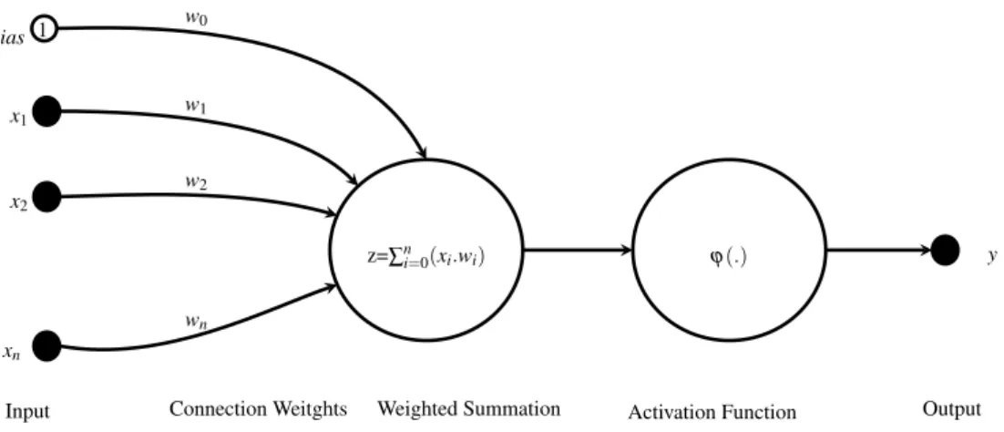
interconnections, called synapses (BISHOP, 2006).
The simplest neural network is composed by just one unit, known as step neuron. It
has a series of inputs(x0,x1, ...,xd), wherex0 represents a bias, whose value is assumed to be always 1, and one output in the form ofy=ϕ(z). For each input a connection weight wi is
defined. The function ϕ is a nonlinear activation function, usually the step function, sigmoid
(Equation 1) or the hyperbolic tangent (Equation 2), andzis a weighted linear combination of its inputs. A general schematic of a neuron is shown in Figure 3.
sigm(z) = 1
1+ez (1)
tanh(z) = e
z−e−z
Input Connection Weitghts Weighted Summation Activation Function Output z=∑n
i=0(xi.wi) ϕ(.)
x1
x2
xn
y w1
w2
wn
bias
w0
1
Figure 3: Example of a neuron, showing the inputs, the weighted sum, the activation function and the output.
Given a dataset X in the form of (xi,yi), where x is the input data and yis the label. Notice that the superscripts denotes each sample in X. The neuron is aimed at finding a nonlinear function f(x), which maps the inputxito its labelyi, for all data samples. Since f(x) is parametrized by the weigths, i.e., f(x,w), the mapping is done by adjusting the connection weights by an iterative learning process. The computation capacity of a single neuron is limited,
being capable of dealing only with small and simple problems.
The solution to real problems requires a more powerful method to find a map, able
to deal with non-linearities. This could be achieved with something like a human brain,
gathering several single neurons into a well defined multilayer structured architecture. It can
be represented as a directed graph of neurons, organized into layers, as shown in Figure 4. The
left-most layer is called input layer, where the input data are introduced into the network. In this
example, the data are represented as a 4-dimensional vector, but the size may vary according to
the application and, especially, to the feature extraction method. The layers in the middle are
denoted as hidden, in the sense that they do not have external inputs or outputs, and all their
neurons are connected to the neurons in the previous layer. The number of neurons in each
layer is a design choice and may vary, especially in accordance with the complexity of the input
data. The right-most layer is the output layer, which is responsible for producing the network
results; and the number of units is related to the expected output (e.g. number of classes). The
architecture details, such as the number of neurons in each layer and the number of layers should
be determined concerning the application.
Formally, the ith neuron within layerl has the form as shown in Equation 3, where i
represents the unit. All units in all layers, except the input layer, operate using this formulation.
This process is called feed-forward, since the data flow is propagated forward throughout the
x1 x2 x3 x4 h1 h2 h3 h4 h5 y1 y2
Input Layer Hidden Layer Output Layer
w1
Figure 4: Example of an multilayer network.
yi,l=ϕ( d
∑
i=1wi,l−1xi,l−1),∀l∈L,∀y∈l (3)
Figure 4 associated to Equation 3, shows that the output of the first hidden layer of an
ANN will be a new representation of the input data concerning to the linear combination with
the connection weights. The weight between x1 and h1 is w1 (solid line). All the remaining weights (dashed lines) are omitted for better visualization. The outputs of the next layers will
lead to a higher representation of the input data. The output of the last layer will be the mapping
between the input data and the desired classes.
Choosing appropriate weight values enables to find arbitrary decisions boundaries,
leading to the desired classification. Theoretically, a three layer neural network could
approximate any function, given the necessary input samples and sufficient hidden units
(BISHOP, 2006).
The common procedure for adjusting the weights of the network is by an interactive
process, where an example is forwarded through the network until an output is obtained. A
cost functionQis used to calculate the difference between the network output and the expected result. In general,Qis defined as Equation 4, and is called mean squared error.
Q(x,w) = 1
2n
∑
x (f(x,w)−y)2
(4)
value ofQ(x,w)must become close to 0. In this way, the weights must be adjusted to minimize the value ofQ(x,w).
A common way to proceed this minimization process is to use the gradient descent
algorithm ( GD). It is based on the partial derivative ∂∂Qw of the cost function with respect to
the weights in the network. This derivative allows to understand how the cost function changes
when the connection weights are changed. Based on this, GD makes small steps in the opposite
direction of the gradient, leading to the consequent minimization ofQ. Equation 5 shows how to update the weights using GD (BISHOP, 2006).
wt=wt−1−η∂Q
∂w, (5)
wheret represents an iteration in the training process, called epoch,η represents the size of the GD step, and is commonly named as learning rate. Choosing the appropriate value
for the learning rate is essential to GD convergence.
It is important to notice that the derivatives must be calculated for every training
sample, and then be averaged before the weight update. This is known asbatchgradient descent. When the training set is big, this process can take a long time, and the learning procedure could
be slow.
Instead of looking at the whole training set, a modification in the procedure updates the
weights after random sampling. This is done using the entire dataset. This is calledstochastic
gradient descent. The calculation in this case is faster than the GD, but the convergence to the
minimum is somewhat random.
Between both there is the mini-batch stochastic gradient descent, in which a small group of training samples are randomly selected and used to update the weights. Again, the
entire dataset is employed. In general, the size of a mini-batch is approximate 100 samples.
This approach is a common choice in the literature.
The process of using the derivative to adjust the weights is called delta learning rule.
A detailed discussion of the backpropagation algorithm can be found in (DUDA et al., 2001;
BISHOP, 2006).
2.4.2 CONVOLUTIONAL NEURAL NETWORKS
The common process for automatic classification, as stated above, is mainly based on
the classification problem. A hand-designed feature extractor requires the presence of a human
expert to find the most suitable data manipulation for achieving good classification performance.
To overcome this, the features could be automatically learnt from the input data. Therefore, the
extractor is adjusted to fit the requirements for a given classification task automatically.
A method conceived to address these characteristics is the CNN, which is a special
type of feed-forward neural network, in whose architecture various hidden layers are employed,
developed to deal with 2D input data, such as images (LECUN et al., 1998).
The main characteristic of this method is the ability to learn a hierarchy of features,
allowing a more abstract representation of the input data. Thus, raw images can be introduced
into the network without any kind of preprocessing or feature extraction. Therefore a trained
CNN is an end-to-end classifier. Another advantage is that the feature extractors are constructed
based on the data used for training, the network learns to manipulate the input data as a way of
performing the classification (LECUN et al., 2010). The architecture of a CNN is designed to
incorporate two modules, as shown in Figure 5: the feature extractor and the classifier.
Figure 5: An example of a CNN architecture. The dashed rectangle denotes the feature extractor layers. The continuous rectangle denotes the classifier layers. The (I) layer represents the raw input image. The (C) layers represent convolution operations. The (S) denotes sub-sampling operations. The linear layers are represented by (L), and (O) represents the output layer.
The feature extractor module is composed by multiple stages, and its inputs and outputs
are called feature maps. Each stage has three different layers: convolution, non-linear filtering
and sub-sampling.
The convolution layer is responsible for storing the trainable weights, which allows
the customization of the feature extractor. The input of a convolution layer is a two-dimension
ml−1 to the output feature mapmli. This connection is performed by a 2D discrete convolution operator using the kernel as the convolution mask.
The trainable kernel is called a receptive field, and the idea is to restrict connections
from a given neuron to a small neighbourhood in the immediately preceding layer, thus forming
a tiny filter for feature extraction. This restriction was inspired by the complex arrangement
of cells within the visual cortex, described by (FUKUSHIMA, 1980). The use of a 2D kernel
allows capturing the spacial relation between adjacent pixels in images.
Since a common feature may be located at different positions in the input image, it
is worth performing the extraction in the entire image. A weight sharing mechanism allows
neurons of the same feature map to have the same weights associated to different receptive
fields. This allows the extraction of features irrespective of the position and reduces the number
of parameters to be trained (LECUN et al., 2010).
The non-linear filtering consists in the application of a non-linear activation function
to all components of each feature map. The reason for that is, as the same as for a regular
neural network, force the network to learn a better representation for the input data, since some
information is lost during the filtering process. The most common choice is the hyperbolic
tangent functiontanh(mli)(LECUN et al., 2010).
The sub-sampling mechanism involves the reduction of a feature map by a constant
factor, providing the network robustness to small distortions and translations. This reduction
is performed over a f1× f2 neighbourhood from the previous layer using a certain operation, such as addition, average and maximum, commonly called maxpooling. For example, if an
input feature map has 28×28 components, and the neighbourhood size is 4×4, the output
feature map will have 7×7 components, being reduced by a factor of 4 (LECUN et al., 1998;
BOUREAU et al., 2010).
Some architectures use a manoeuvre to give the network some translation invariance
and reduce the computation effort. Instead of applying a convolution kernel or sub-sampling
operation to every possible location on the input map, leading to an overlapping region, a stride
is used. This means that a step, in both horizontal and vertical directions, is used.
The last module of a CNN consists in the classifier itself. Its inputs are the outputs
from the last feature maps. In general, a common linear feed-forward classifier is employed.
The amount of input neurons, hidden layers and output neurons is problem-dependent.
To adjust the weights of the network, a variation of the backpropagation learning
way, seeking to reduce the error between the predicted and the expected results, generally using
the stochastic gradient descent ( SGD) algorithm.
2.4.3 LENET – 5
The concepts discussed above were first applied to document recognition, more
specifically, to handwritten character recognition (LECUN et al., 1998). In that paper, an
architecture for a CNN, called LeNet-5, was proposed and tested. This network became the
ground basis for further research about CNN.
The network, as shown in Figure 6, comprises 7 layers, not including the input. The
input to the CNN is a 32×32 black and white image. LayerC1 is a convolutional layer with 6×28×28 feature maps generated by a 5×5 trainable kernel. LayerS2 reduces theC1 feature maps to 6×14×14, using a 2×2 neighbourhood. The four inputs to a unit inS2 are added, then multiplied by a trainable coefficient, and added to a trainable bias. The result is squashed
by a sigmoid function. LayerC3 is a convolutional layer with 16 feature maps of size 10×10, generated by 5×5 trainable kernels. UnlikeC1, theC3 layer has a special form of connection between its feature maps and theS2 maps. This was proposed to reduce the number of network parameters and increase its capacity. LayerS4 reduces the 16 feature maps fromC3 to 5×5, using the same operation asS2. LayerC5 processes the 16 feature maps fromS4 using 5×5 trainable kernels. Because the S4 maps have a size of 5×5, the output ofC5 is 120 feature maps of size 1×1. The next layer,F6, is a linear, or fully-connected layer, and acts as a layer in an MLP network, computing the linear combination of its inputs with trainable weights. Output
layerF7 is composed of Euclidean Radial Basis Function units (RBF), one for each class, with 84 inputs each. The whole LeNet-5 has a total number of 14,000 trainable parameters (LECUN
et al., 1998).
Figure 6: LeNet-5 network architecture, which was proposed to classify handwritten digits.
The network was trained and tested using the MNIST handwritten digits database.
The training procedure used 60,000 samples while the test set was composed of 10,000 images.
After 20 passes through the training database, the network achieved an error of 0.95% on the test
set. When an expanded version of the training database was employed, the test error dropped
to 0.8%. The expansion was created using distortions in the images, such as horizontal and
vertical translations, scaling, squeezing and horizontal shearing.
2.4.4 USAGE OF CNN
Despite the fact that the first CNN was proposed a long time ago, it attracted much
attention in recent years. The community claims that two major facts reactivated research on this
topic: the popularization of the use of powerful Graphical Processing Units ( GPUs), along with
the tools to develop algorithms using this technology, such as the Nvidia’s CUDA framework;
and the availability of huge annotated image databases, such as the ImageNET (DENG et
al., 2009). This has led to numerous methodological proposals for different issues related to
CNN, including the use of unsupervised pre-training, activation units, training procedures and
architectures.
(KRIZHEVSKY et al., 2012) proposed a CNN architecture as a solution to the
ImageNet Large Scale Visual Recognition Challenge 2010 (ILSVRC2010), where 1.2 million
high-resolution images had to be classified into 1000 different classes. The network was
composed of eight learned layers: five convolutional and three fully-connected, as shown in
Figure 7. The first layer transforms a 224×244 RGB image into 96 feature maps using kernels
with 11×11×3 components and a 4-pixel distance (stride) between the receptive fields. The
second layer expands the output of layer one to 256 feature maps, where the kernel has 5×5×48
components. The third layer has 384 feature maps generated by kernels of size 3×3×256. The
fourth layer has 384 maps generated by kernels with a size of 3×3×192. The fifth layer has
384 maps generated by kernels of size 3×3×192. The fully-connected layers have 4096
units each. The max-pooling and a local normalization operation are employed only after the
first and second layer. This architecture has 650,000 processing units and 60 million trainable
parameters.
The training process of such a large network demands high computation power. A
multi-GPU scheme was employed to adjust the network parameters in between five and six
days. This optimization scheme unveils an affordable platform for training large CNNs.
During the training phase, the units in the fully-connected hidden layers of the CNN
Figure 7: CNN architecture proposed by (KRIZHEVSKY et al., 2012) as solution to ILSVRC2010.
Source: Adapted from (KRIZHEVSKY et al., 2012)
given input. If the number of hidden units is large, the units can learn very well how to classify
the entire training data set. But when the network is used to predict the class of new input data,
the results may be worst. This phenomenon is called overfitting. A possible way of reducing
the overfitting, as proposed by (SRIVASTAVA et al., 2014), is to randomly turn off hidden units
with a probability of 1/2 during the training phase.
The algorithm consists in, for each training example and training epoch, randomly
chosen hidden units are selected and temporary deleted. The other remaining weights are
normally trained using backpropagation (BALDI; SADOWSKI, 2014). Figure 2.4.4 shows a
representation for this process, where light circles and dashed lines represent turned off units.
This procedure is called dropout learning.
Figure 8: Representation of how dropout works.
Source: Adapted from (BALDI; SADOWSKI, 2014)
This procedure can produce two main advantages in the neural network behaviour.