Faculty of Engineering of the University of Porto
Development of a new computational approach
to simulate blood flow
Mariana Sousa Santos
Dissertation carried out under the
Integrated Master in Bioengineering
Major Biomedical Engineering
Supervisor: Jorge Belinha, PhD
Co-Supervisor: Renato Natal Jorge, PhD
ii
iii
Abstract
Cardiovascular diseases are a leading cause in mortality worldwide. Diseases like atherosclerosis and aneurysms disturb the blood flow, leading to clinical complications. The simulation of blood flow is very important to understand the function of the cardiovascular system under normal and abnormal conditions, designing cardiovascular devices, and diagnosing and treating disease.[1] This process has been studied, however, in certain types of blood vessels, like veins, there are few studies.
This project proposes to simulate blood flow using a fully developed meshless method software in two dimension (2D) models and three dimension (3D) models. In opposition to the Finite Element Method (FEM), meshless methods are new discrete numerical methods much more flexible and accurate. Thus, to determine the velocity field, a numerical tool is required. In this work two meshless numerical methods are used, the Radial Point Interpolation Method (RPIM) and the Natural Neighbour Radial Point Interpolation Method (NNRPIM). The velocity profiles and the discharge are used to compare the numerical methods. In end, it is expected to conclude if meshless methods are suited to explicitly simulate blood flow.
For this work, the blood was simulated being a Newtonian fluid, since in large vessels, the non-Newtonian effects are not significant. The work analysed six different 2D models, representing different possible geometries for vessels, and three 3D models, showing different geometries. In the end, several benchmark examples were extracted from literature and compared with FEM and meshless methods. The results show that the meshless methods are suited to simulate blood flow.
v
Resumo
As doenças cardiovasculares são uma das principais causas de mortalidade no mundo. Doenças como a arteriosclerose e aneurismas causam um distúrbio no fluxo sanguíneo, levando a complicações clínicas. A simulação do fluxo sanguíneo é então muito importante para perceber a função do sistema cardiovascular sobre condições normais e patológicas, desenhar dispositivos cardiovasculares, e diagnosticar e tratar patologias. [1] Este processo já tem vindo a ser estudado, no entanto, em certos tipos de vasos, como veias, ainda existem poucos estudos.
Este projeto propõe simular o fluxo sanguíneo usando um software de métodos numéricos sem malha em modelos a duas dimensões (2D) e a três dimensões (3D). Em oposição ao método dos elementos finitos (MEF), os métodos sem malha são novos métodos numéricos discretos muito mais flexíveis e precisos. Portanto, é necessário utilizar uma ferramenta numérica para determinar o campo de velocidades. Neste trabalho dois métodos numéricos irão ser usados, o
Radial Point Interpolation Method (RPIM) e o Natural Neighbour Radial Point Interpolation Method (NNRPIM). Os perfis de velocidades e os caudais são usados para comparar os métodos
numéricos. No final, é esperado concluir se os métodos sem malha são adequados para explicitamente simular o fluxo sanguíneo.
Neste trabalho, o sangue foi simulado sendo um fluido Newtoniano, visto que em vasos de alto calibre os efeitos não-Newtonianos são desprezíveis. Este trabalho analisa seis modelos 2D diferentes, representando diferentes geometrias para vasos, e três exemplos 3D, representando diferentes geometrias. No fim, vários exemplos de referência foram retirados da literatura e comparados com FEM e os métodos numéricos sem malha. Os resultados mostram que os métodos sem malha são adequados para simular o fluxo sanguíneo.
vii
Acknowledgements
Um muito obrigado ao orientador, o Professor Jorge Belinha por todo o tempo que dispensou a ajudar-me e por estar sempre pronto a esclarecer quaisquer dúvidas que tivesse.
Estes cinco anos na Faculdade de Engenharia, a qual foi a minha segunda casa, não tinham sido tão fantásticos se não fossem as pessoas que encontrei pelo caminho. Por isso, um grande obrigado os amigos de Bioengenharia que me acompanharam ao longo do tempo.
Um grande obrigado também ao BEST Porto, por todo o crescimento que me proporcionou, em especial neste último ultimo ano em que tive o prazer de fazer parte da XXI direção. Queria agradecer em especial ao management da associação, por estar sempre presente neste ultimo ano, que sem dúvida tem tido muitos desafios.
Um grande obrigado aqueles que me ajudaram a chegar até aqui, os meus pais, que sempre apoiaram as minhas decisões.
ix
Institutional acknowledgements
The author truly acknowledges the work conditions provided by the Applied Mechanics Division (SMAp) of the department of mechanical engineering (DEMec) of FEUP and by the inter-institutional project “BoneSys – Bone biochemical and biomechanic integrated modeling: addressing remodeling, disease and therapy dynamics” funded by the “Laboratório Associado de Energia Transportes e Aeronáutica” (UID/EMS/50022/2013) and by the project NORTE-01-0145-FEDER- 000022 – SciTech – Science and Technology for Competitive and Sustainable Industries, co-financed by Programa Operacional Regional do Norte (NORTE2020), through Fundo Europeu de Desenvolvimento Regional (FEDER).
xi
“We choose to go to the Moon! ... We choose to go to the Moon in this decade and do the other things, not because they are easy, but because they are hard; because that goal will serve to organize and measure the best of our energies and skills, because that challenge is one that we are willing to accept, one we are unwilling to postpone, and one we intend to win ...”
xiii
Table of contents
Abstract ... iii
Resumo ... v
Acknowledgements ... vii
Institutional acknowledgements ... ix
Table of contents ... xiii
List of figures ... xv
List of Tables ... xxi
Abbreviations and symbols ... xxiii
Chapter 1 ... 1
Introduction ... 1 1.1 - Motivation ... 1 1.2 - Objectives ... 2 1.3 - Document Structure ... 2Chapter 2 ... 1
Blood Flow ... 12.1 - Biological description of circulation ... 1
2.2 - Blood constitution ... 2
2.3 - Mechanical properties ... 3
2.4- Constitutive/rheological models to simulate blood ... 4
Chapter 3 ... 7
xiv
3.1 - Finite element method ... 7
3.2 - Meshless method ... 7
3.2.1. General meshless method procedure ... 8
3.2.2. RPIM Formulation ... 9
4.2.3- NNRPIM Formulation ... 12
3.3 - Discretized formulation flow ... 17
3.4 - Numerical analysis applied to blood flow ... 20
Chapter 4 ... 23
Preliminary studies ... 23
4.1- 2D convergence studies ... 23
4.1.1- Linear model ... 26
4.1.2- Crescent cone model ... 35
4.1.3- Cone decrescent model ... 44
4.1.4- Quarter of a circular crown model ... 54
4.1.5- Half of a circular crown model ... 63
4.1.6- Double curve model ... 75
4.2- 3D studies ... 82
4.2.1- Linear model ... 83
4.2.2- Quarter of a crown model ... 88
4.2.3- Double curve model ... 93
4.2.4- General remarks ... 97
Chapter 5 ... 99
Case studies ... 99
5.1 -Comparison with another constitutive model for blood ... 99
5.2 -Bifurcation ... 101
5.3 -Spastic middle cerebral arteries ... 104
5.4 -Cerebral aneurysm ... 108
5.5 -Aortic aneurysm ... 109
5.6 -Real bifurcation ... 112
Chapter 6 ... 113
Conclusions and future work ... 113
xv
List of figures
Figure 2.1 - Human blood viscosity as a function of shear rate for a range of hemaocrit concentrations on a log-log plot [21][22][23][19] ... 4 Figure 2.2 - The non-Newtonian fluid models that are commonly used to describe blood
rheology [19] ... 5 Figure 3.1 - a. Problem domain with the essential and natural boundaries applied. b.
Regular nodal discretization. c. Irregular nodal discretization.[40] ... 8 Figure 3.2 – a. Fixed rectangular shaped influence-domain. b. Fixed circular shaped
influence-domain. c. Flexible circular shaped influence-domain [40] ... 9 Figure 3.3 - a. Fitted Gaussian integration mesh. b. General Gaussian integration mesh. c.
Voronoï diagram for nodal integration [40] ... 10 Figure 3.4 – a. Initial quadrilateral from the grid-cell. b. Transformation of the initial
quadrilateral into an isoparametric square shape and application of the 2 x 2 quadrature point rule. c Return to the initial quadrilateral shape [40] ... 10 Figure 3.5 – a. Initial nodal set of potential neighbour nodes of node 𝑛0. b. First trial
plane. c. Second trial plane. d. Final trial cell containing just the natural neighbours of node 𝑛0. e. Node 𝑛0 Voronoï cell 𝑉0. f. Voronoï diagram [40] ... 12 Figure 3.6 - a. First degree influence-cell b. Second degree influence-cell [40] ... 14 Figure 3.7 – a. Voronoï diagram, b. Delaunay triangulation and c. Natural neighbour
circumcircles [40] ... 14 Figure 3.8 - Triangular shape and quadrilateral shape and the respective integration points
𝑥𝐼 using the Gauss-Legendre integration scheme [40] ... 15 Figure 3.9 – Finite Element and Meshless Analysis Software (FEMAS) - Print-screen of an
xvi
Figure 4.1 – Laminar velocity profile in a tube [45] ... 24
Figure 4.2 – Example of the boundary conditions applied ... 25
Figure 4.3- Representation of the nodes in a cross section ... 26
Figure 4.4 – Linear model with different meshes ... 27
Figure 4.5 – Linear model (21 nodes) analysed with different methods ... 28
Figure 4.6 – Linear model (65 nodes) analysed with different methods ... 29
Figure 4.7 – Linear model (255 nodes) analysed with different methods... 30
Figure 4.8 – Linear model (833 nodes) analysed with different methods... 31
Figure 4.9 – Linear model (3201 nodes) analysed with FEM (triangular elements with 6 nodes) ... 32
Figure 4.10 - Discharge in every cross section of the models ... 32
Figure 4.11 – Discharge in each cross session with different methodologies ... 34
Figure 4.12 – Velocity profiles in each cross session with different methodologies ... 35
Figure 4.13 – Crescent cone model with different meshes ... 36
Figure 4.14 – Cone crescent model (21 nodes) analysed with different methods... 37
Figure 4.15 – Cone crescent model (65 nodes) analysed with different methods... 38
Figure 4.16 – Cone crescent model (255 nodes) analysed with different methods ... 39
Figure 4.17 – Cone crescent model (833 nodes) analysed with different methods ... 40
Figure 4.18 - Cone crescent model (3201 nodes) analysed with FEM (triangular elements with 6 nodes) ... 41
Figure 4.19 - Discharge in every cross section of the models ... 41
Figure 4.20 – Discharge in each cross session with different methodologies ... 43
Figure 4.21 – Velocity profiles in each cross session with different methodologies ... 44
Figure 4.22 – Decrescent cone model with different meshes ... 45
Figure 4.23 – Cone decrescent model (21 nodes) analysed with different methods ... 46
Figure 4.24 – Cone decrescent model (65 nodes) analysed with different methods ... 47
xvii
Figure 4.26 – Cone decrescent model (833 nodes) analysed with different methods ... 49
Figure 4.27 – Cone decrescent model (3201 nodes) analysed with FEM (triangular elements with 6 nodes)... 49
Figure 4.28 - Discharge in every cross section of the models ... 50
Figure 4.29 – Discharge in each cross session with different methodologies ... 52
Figure 4.30 – Velocity profiles in each cross session with different methodologies ... 53
Figure 4.31 – Quarter of a circular crown model with different meshes ... 54
Figure 4.32 – Quarter of a circular crown model (21 nodes) analysed with different methods ... 55
Figure 4.33 – Quarter of a circular crown model (65 nodes) analysed with different methods ... 56
Figure 4.34 – Quarter of a circular crown model (255 nodes) analysed with different methods ... 57
Figure 4.35 – Quarter of a circular crown model (833 nodes) analysed with different methods ... 58
Figure 4.36 – Quarter of a circular crown model (3201 nodes) analysed with FEM (triangular elements with 6 nodes) ... 59
Figure 4.37 - Discharge in every cross section of the models ... 59
Figure 4.38 - Cross sections ... 60
Figure 4.39 – Discharge in each cross session with different methodologies ... 61
Figure 4.40 – Velocity profiles in each cross session with different methodologies ... 63
Figure 4.41 – Distortion of the axial velocity profile as a result of tube curvature [47] ... 63
Figure 4.42- Half of a circular crown model with different meshes ... 64
Figure 4.43 – Half of a circular crown model (75 nodes) analysed with different methods .. 66
Figure 4.44 – Half of a circular crown model (125 nodes) analysed with different methods ... 66
Figure 4.45 – Half of a circular crown model (441 nodes) analysed with different methods ... 67
Figure 4.46 – Half of a circular crown model (1659 nodes) analysed with different methods ... 68
xviii
Figure 4.47 - Discharge in every cross section of the models ... 69
Figure 4.48 – Cross sections in half of a crown model ... 69
Figure 4.49 – Velocity profiles in each cross session with different methodologies ... 72
Figure 4.50 – Discharge in each cross session with different methodologies ... 74
Figure 4.51 Double curve model with different meshes ... 75
Figure 4.52 – Double curve model (75 nodes) analysed with different methods ... 76
Figure 4.53 – Double curve model (245 nodes) analysed with different methods ... 77
Figure 4.54 – Double curve model (873 nodes) analysed with different methods ... 78
Figure 4.55 – Double curve model (3281 nodes) analysed with different methods ... 79
Figure 4.56 - Cross sections in the double curve model ... 79
Figure 4.57 - Discharge in every cross section of the models ... 80
Figure 4.58 – Velocity profiles in each cross session with different methodologies ... 81
Figure 4.59 – Discharge in each cross session with different methodologies ... 82
Figure 4.60 – Linear 3D model ... 83
Figure 4.61 – Linear 3D model FEM analysis ... 85
Figure 4.62 – Linear 3D model FEM analysis – cross section views ... 85
Figure 4.63 – Linear 3D model NNRPIM analysis ... 86
Figure 4.64 – Linear 3D model NNRPIM analysis ... 86
Figure 4.65 – Linear 3D model RPIM analysis ... 87
Figure 4.66 – Linear 3D model NNRPIM analysis ... 87
Figure 4.67 – Quarter circular crown model ... 88
Figure 4.68 – Quarter circular crown model analysed with FEM ... 90
Figure 4.69 – Quarter circular crown model analysed with NNRPIM ... 91
Figure 4.70 – Quarter circular crown model analysed with RPIM ... 92
Figure 4.71 – Double curve model ... 93
xix
Figure 4.73 – Double curve model analysed with RPIM ... 95
Figure 4.74 – Double curve model analysed with RPIM ... 96
Figure 5.1 – Velocity field for the Carreau model for inlet centre line velocities of 0.8 m/s [48] ... 99
Figure 5.2 – Reproduced model ... 100
Figure 5.3 – Comparison in [48] between the velocity profiles expected ... 100
Figure 5.4 – Numerical analysis of model ... 100
Figure 5.5 – Bifurcation models ... 101
Figure 5.6 – Numerical analysis of model with the initial constant velocity ... 103
Figure 5.7 – Numerical analysis of model with the parabolic initial velocity ... 104
Figure 5.8 – Results presented in literature ... 105
Figure 5.9 – Numerical analysis of model ... 107
Figure 5.10 – Numerical analysis of model ... 107
Figure 5.11 – Results presented in paper ... 108
Figure 5.12 – Numerical analysis of model ... 109
Figure 5.13 – Results presented in paper ... 110
Figure 5.14 – Numerical analysis of model ... 111
xxi
List of Tables
Table 2.1 – Human blood composition [18] ... 2
Table 4.1 – Default RPIM and NNPIM used in the analysis ... 25
Table 4.2 – RPIM and NNRPIM parameters in the linear 3D model ... 84
Table 4.3 – RPIM and NNRPIM parameters in the quarter circular crown 3D model ... 89
Table 4.4 – RPIM and NNRPIM parameters in the half circular crown 3D model ... 94
Table 5.1 – RPIM and NNRPIM parameters in the bifurcation model with constant velocity profile ... 102
Table 5.2 – RPIM and NNRPIM parameters in the bifurcation model with parabolic velocity profile ... 102
Table 5.3 – RPIM and NNRPIM parameters in the spastic middle cerebral artery model (a) .. 105
Table 5.4 – RPIM and NNRPIM parameters in the spastic middle cerebral artery model (b) . 106 Table 5.5 – RPIM and NNRPIM parameters in cerebral aneurism ... 108
xxiii
Abbreviations and symbols
List of abbreviations
DVT Deep Venous Thrombosis FEM Finite Element Methods
FEMAS Finite Element and Meshless Analysis Software FPM Finite Point Methods
MLPG Meshless Local Petrov-Galerkin
MQ Multiquadric
NNRPIM Natural Neighbor Radial Point Interpolation Method RPIM Radial Point Interpolation Method
RBF Radial Basis Functions RPI Radial Point Interpolation RPIM Real Property Information Model SPH Smooth Particle Hydrodynamics CVD Cardiovascular diseases List of symbols 𝛼 penalty factor 𝛾 fluidity parameter 𝛿 Identity matrix 𝜀 strain 𝜇 viscosity 𝜌 density 𝜎 stress 𝜏 torsion
𝜔 weight of the integration points 𝛾̇ shear rate
xxiv 𝛾̇𝑐 characteristic shear rate
𝜸̇ rate of strain tensor
λ characteristic time constant λ1 relaxation time λ2 retardation time µ fluid viscosity µp plasma viscosity µ0 zero-shear-rate viscosity µ∞ infinite-shear-rate viscosity τ τ shear stress τ stress tensor
τc characteristic shear stress
τo yield-stress
Φ volume concentration a Carreau-Yasuda index k consistency coefficient
k0 maximum volume fraction for zero shear rate
k∞ maximum volume fraction for infinite shear rate
m Cross model index
n power law index
Chapter 1
Introduction
1.1 - Motivation
The cardiovascular system and its well function is vital for human beings to carry their daily lives. But, despite the development in healthcare systems over the past few decades, cardiovascular disease is still a worrying problem.
Cardiovascular disease (CVD) is the leading cause of death worldwide[2], accounting for one-third of global deaths. [3] Just in Europe, CVD causes 3.9 million deaths and over 1.8 million deaths in the European Union (EU).[4]
Besides the mortality, there are several life conditions that can affect the quality of life of people with chronic CVD.[5][6][7] This results in substantial disability and loss of productivity and contributes to the escalating costs of health care.[4]
Due to the aging population and to classical risk factors, namely diets high in saturated fats, elevated serum cholesterol and blood pressure (BP), diabetes, and smoking, [8] in 2015, more than 85 million people in Europe were living with CVD and almost 49 million people were living with CVD in the EU. [4]
Overall CVD is estimated to cost the EU economy €210 billion a year. Of the total cost of CVD in the EU, around 53% (€111 billion) is due to health care costs, 26% (€54 billion) to productivity losses and 21% (€45 billion) to the informal care of people with CVD.[4]
The aging population and the unhealthy habits have brought some challenges to the national health systems from all over the world, so it is necessary to develop strategies to make prevention, diagnosis and treatment more efficient.
The simulation of blood flow is very important to understand the function of the cardiovascular system under normal and abnormal conditions, designing cardiovascular devices, diagnosing and treating disease.[1] It is established that blood disturbances can lead to clinical complications in areas of complex flow, like in coronary and carotid bifurcations or stenosed arteries. [9] This methods allow, in a non-intrusive virtual manner, the estimation of a multitude of blood flow characteristics.[10]
There are some cases where this study can be important. Cerebral aneurysm rupture, leading to subarachnoidal hemorrhage accounts for approximately 7% of all strokes. [10] Aortic aneurysms are a main cause of death in the elderly population throughout the western world [11] and deep vein thrombosis is also the leading cause of preventable hospital death[12], [13] and a leading cause of maternal mortality in the U.S. [14] Coronary heart disease caused by
2 Introduction
2
atherosclerosis is the major cause of mortality from cardiovascular disease in much of the world’s population, which is the leading cause of death in the United States[15][16]
Understanding how the blood flow works in several situations has been studied with several numerical methods, however, the study with meshless methods is still much unexplored. Hence this thesis aims to create a reliable biomechanical simulation of the blood flow with RPIM and NNRPIMM.
1.2 - Objectives
The main objective of this project is to develop a new computational approach to simulate blood flow.
Therefore, to accomplish this goal, several secondary objectives were stipulated, such as:
Perform a steady flow analysis of the blood flow, using the two of the most recent meshless models nowadays, the RPIM and NNRPIM;
Study the effect of different geometries in the velocity map of blood flow
Draw comparisons between FEM and the meshless methods used.
1.3 - Document Structure
This thesis is composed of seven major chapters: Introduction, Blood Flow, Numerical methods, The modelling and analysis process, Preliminary studies, Case studies and Conclusions and future work.
In Chapter 1, Introduction, a brief introduction and the motivation to carry this work is explained. The goals of this work are as well stated in this chapter.
In Chapter 2, Blood Flow, a biological description of the cardiovascular system, the blood constitution and its mechanical properties is given and different constitutive and rheological models to simulate blood.
In Chapter 3, Numerical methods, it is explained the two meshless methods in this work and the flow formulation for viscoplastic materials used in this work.
In Chapter 4, Preliminary studies, it is performed a study to compare the different numerical methods, different levels of discretization and different geometries. Afterwards, it was performed a 3D study with the three methods.
In Chapter 5, Case studies, some examples found in scientific papers are reproduced and compared with the results from FEM and meshless methods.
In Chapter 6, Conclusions and future work, the main conclusion of this work is presented and some recommendations for future work in the topic are given.
Chapter 2
Blood Flow
2.1 - Biological description of circulation
The circulatory system is a system that permits blood to circulate and transport essential molecules for the well-functioning of the human body. It needs to provide adequate continuous flow and regulate it according the body needs [17]. The cardiovascular system consists of the heart, blood vessels and blood.
The heart is a muscle pumping blood throughout the entire cardiovascular system. It is composed of two separate pumps that work to transport blood through the vascular system. One of these pumps (left side) delivers oxygenated blood to the body, while the other pump (right side) delivers deoxygenated blood to the lungs. [18]
The vasculature consists of arteries, arterioles, capillaries, venules and veins. The vasculature is normally divided into two parts: the pulmonary and systemic circulations. The network of blood vessels from the right heart to the lungs and back to the left heart is referred to as the pulmonary circulation system and the rest of the blood flow loop is called systemic circulation system. Blood is pumped at a rate of 5,2 litres per minute[17].
The blow flows through large arteries, then branches into smaller arteries, before reaching arterioles and capillaries. After capillaries, and before reaching the right heart, the blood enters the venules before joining smaller veins first and then larger veins. The pressure gradient developed between the arterial and the venous end of the circulation is the driving force causing blood flow through the blood vessels.[17]
The main functions of the cardiovascular system are the distribution of oxygen (acquired from the lungs) and nutrients (acquired from the intestine) to the cells in all parts of the body, elimination of cellular wastes and carbon dioxide from the cells (excreted through the kidneys) and maintain the thermostasis.[17]
2 Blood Flow
2
2.2 - Blood constitution
Blood is composed of two major components: the cellular component and the plasma component (see Table 2.1). In an average adult, the blood volume is approximately 5 L, of which approximately 55% to 60% is plasma and the remaining portion is cellular. More than 99% of the cellular component is composed of red blood cells. [18] The remaining portion of the cellular volume (less than 1%) is composed of white blood cells and platelets.
Table 2.1 – Human blood composition [18] Cellular Component (~ 40%) Cell type Cell concentration Characteristic Shape/Dimensions Red Blood Cell
(Erythrocyte - ~99.7%) ~5,000,000/μL
Biconcave Discs 8 μm Diameter 2.5 μm Thickness White Blood Cell
(Leukocyte - ~0.2%) ~7,500/μL Spherical 20-100 μm Diameter Platelet (Thrombocyte - ~0.1%) ~250,000/μL Ellipsoid 4 μm Long Axis 1.5 μm Short Axis Plasma component (~ 60%) Composition Major contributors Function
Water (~92%) H2O Reduce Viscosity
Plasma Proteins (~7%) Albumin ( ~60%) Globulins (~35%) Fibrinogen (~3%) Others (~2%) Osmotic Pressure Immune Function Clotting Enzymes/Hormones Other Solutes (~1%) Electrolytes Nutrients
Wastes
Homeostasis Cellular Energy
Excretion Red blood cells (or erythrocytes) are responsible for the delivery of oxygen and the removal of carbon dioxide from all cells of the body through hemoglobin and the maintenance of the blood pH, using hemoglobin as a buffer. The shape of red blood cells can change for these cells to squeeze through capillaries. [18]
White blood cells (or leukocytes) are the primary cells that protect the body from foreign particles. They can directly destroy foreign particles or produce antibodies that aid in the immune response. There are six types of white blood cells (neutrophils, lymphocytes, monocytes, eosinophils, basophils, and plasma cells) in the body, each with its own specialized function. [18]
Of those cells, neutrophils account for more than 60% of them, lymphocytes account for approximately 30%, monocytes account for approximately 5%, eosinophils account for approximately 2.5%, basophils account for 0.5%, and plasma cells approximately 0.1%. [18]
Platelets (or thrombocytes) are the primary cells for hemostasis. They are cellular fragments of megakaryocytes, which are derived from hematopoietic stem cells. Platelets do not contain nuclei or many of the other common cellular organelles, and contain anti-thrombotic proteins that cleave activated zymogens. The shear stress can alter the platelet physiology significantly. Under disturbed blood flow conditions (e.g., high shear stresses, recirculation zones, oscillating stresses), platelets may accelerate cardiovascular disease progression. [18] An abnormal number of platelets can lead to coagulation problems.
3
Plasma is the second major component of blood. Its main composition is water, electrolytes, sugars, urea, phospholipids, cholesterol, and proteins. [18]
Approximately 2% of this is accounted for by sugars within the plasma. Cholesterol contributes 4% to 5% of those (in a normal diet) and phospholipids are approximately 6% to 7% of those. Proteins account for 7% of the total composition of plasma. The most crucial and most abundant protein within the blood is albumin, which accounts for over 60% of the total plasma protein concentration. Albumin has the primary function of maintaining the osmotic pressure of blood. It acts to balance the mass transfer across the capillary wall. Antibodies play a role in immunology and transport globulins can bind to hormones, metallic ions, and steroids, among others, to transport these molecules throughout the body. The remaining plasma protein composition is made up of fibrinogen (approximately 3%) and all the other proteins. Fibrinogen is the precursor to fibrin and forms a mesh during clot formation. [18]
In general, the water portion of plasma is used to reduce the viscosity of the cellular component of blood, reducing the flow resistance and allowing blood flow to occur. A major function of the remaining plasma components is to maintain equilibrium with the interstitial space, which aids in homeostasis. Sugars are used as the nutrient source for cells. Cholesterol can be used within the cell membrane to increase its rigidity so the cell can withstand forces better. Proteins have specific functions and each protein may have a different task. Therefore, plasma has a very critical function for the human body. [18]
2.3 - Mechanical properties
Blood is a special non-Newtonian fluid that is also composed of at least two phases. The rheological characteristics of blood are determined by all its properties and their interaction with each other, as well as with the surrounding structures. The properties of a non-Newtonian fluid include deformation rate dependency, viscoelasticity, yield stress and thixotropy. Most non-Newtonian effects originate from red blood cells due to their high concentration and distinguishes mechanical properties such as elasticity and ability to aggregate forming three-dimensional structures at low deformation rates. [19]
Blood is a thixotropic fluid because its apparent viscosity decreases under a constant shear stress. [18]
Non-Newtonian effects in general are seen in certain flow regimes, such as low shear rates and are influenced by the type of deformation.[19]
Blood is a predominantly shear thinning fluid, especially under steady flow conditions. At low shear rates or shear stresses the apparent viscosity is high, whereas the apparent viscosity decreases with increasing shear. [20]
Yield stress contributes to the blood clotting following injuries and subsequent healing, and may also contribute to the formation of blood clots (thrombosis) and vessel blockage in some pathological cases such as strokes.[19]
The viscosity of whole blood varies with shear rate, haematocrit (see Figure 2.1), temperature, and disease conditions, and this is predominantly due to the presence of cells and other compounds within the fluid.[18]
4 Blood Flow
4
Figure 2.1 - Human blood viscosity as a function of shear rate for a range of hemaocrit concentrations on a log-log plot [21][22][23][19]
At stasis, normal blood has a yield stress of about 2 to 4 mPa [24][20]. The value of blood viscosity ranges from 3.01 to 5.53 cP [17], corresponding to 3.01 to 5.53 mPa.s, and has a density 1060 kg/m3[25][26].
These values result from experimental studies. There are several models that can modulate the behaviour of blood. The model used will be presented later in the chapter “Numerical analysis of blood and coagulation”.
2.4- Constitutive/rheological models to simulate blood
As discussed before, blood is a non-Newtonian fluid. In literature, there were several models used including Carreau-Yasuda, Casson, power law, Cross, Herschel, Oldroyd-B, Quemada, Yeleswarapu, Bingham, Eyring-Powell, and Ree-Eyring. The more frequent used models are Casson and Carreau-Yasuda models. [19]
Blood can be modulated as a Newtonian fluid, which can be applied in large vessels at medium and high shear rates under non-pathological conditions. This is due to the fact that blood is exposed to relatively high shear rates and non-Newtonian effects are induced at low shear rates (<100 s-1). In the venous part of the circulatory system, the Newtonian effects are more significant than in the arterial part due to low deformation rates.[19]
None of the mentioned models are capable to reproduce accurately all the features and properties of blood flow.[44]
The Figure 2.2 represents the equations of the rheological models and the non-Newtonian properties that are used in literature to simulate the blood flow.
5
Figure 2.2 - The non-Newtonian fluid models that are commonly used to describe blood rheology [19]
The symbols present in Figure 2.2 - are the following: 𝛾̇ shear rate
𝛾̇𝑐 characteristic shear rate
𝜸̇ rate of strain tensor
λ characteristic time constant λ1 relaxation time λ2 retardation time µ fluid viscosity µp plasma viscosity µ0 zero-shear-rate viscosity µ∞ infinite-shear-rate viscosity τ τ shear stress τ stress tensor
τc characteristic shear stress
τo yield-stress
Φ volume concentration a Carreau-Yasuda index k consistency coefficient
k0 maximum volume fraction for zero shear rate
k∞ maximum volume fraction for infinite shear rate
m Cross model index
n power law index
∇ upper convected time derivative
In this work, the focus were large vessels so, the Newtonian formulation of blood flow was used. Other limitations were found while trying to explore the models mentioned earlier, such as the kind of formulation allowed in the software used and lack of information on the values of the variables to fit the models.
where 𝜇 is the viscosity coefficient.
6 Blood Flow
Chapter 3
Numerical methods
3.1 - Finite element method
Today, the finite-element method is very used in industry and biomechanics [27], in simulating deformable models and flow [28]. In fluid analysis is particularly useful in surgical simulation.
The technique consists in dividing the flow domain into smaller regions (elements), in which governing equations are applied. These equations are rewritten in algebraic form to represent the changes that occur in variables due to incremental changes in position and time. These solutions are adapted each cycle over the entire mesh until a converged value for the viscosity is achieved. The time of the analysis depends on the geometry, mesh configuration and boundary conditions imposed. The major advantage of the FEM is the discretization procedure for simple geometric shapes.[17]
However, mesh-based algorithms, when faced with complex models, irregular geometries, or analyses dealing with large deformations (such as fluid flow), require significant amounts of computation in remeshing tasks.
Applied to fluid mechanics, in the 70’s there were published the first FEM articles for the Navier-Stokes equations (Chung[29] ,Temam[30], Thomasset[31]).[28]
To try to overcome the problem of high computation time, in recent years, several algorithms were developed for 3D flows (multigrid, (Brandt[32], Hackbush[33]), domain decomposition (Glowinski[33]), vectorization (Woodward et al[34]), the development of specialized methods to reach certain objectives (spectral methods, (Orszag[35]), particle methods (Chorin [36]). [28]
3.2 - Meshless method
The problems associated with FEM have created the need to develop a numerical technique capable of reducing the computational time. Meshless methods are used to analyse more complex physics on a set of non-ordered points. These methods were proved to be valid in solid mechanics, fluid dynamics and heat transfer.[37], [38]
8 Numerical methods
8
There are several types of meshless methods used in fluid dynamics, including Smooth Particle Hydrodynamics (SPH), the Meshless Local Petrov-Galerkin (MLPG) method, methods based on Radial Basis Functions (RBF), and Finite Point Methods (FPM).[39]
This work will be developed using two of the most recently developed meshless methods: the Radial Point Interpolation Method (RPIM) and the Natural Neighbour Radial Interpolation Method (NNRPIM). In this chapter, after a brief description of the general meshless method procedure, both methods are presented and thoroughly explained. The chapter ends with the presentation of the radial point interpolation (RPI) shape functions, which construction procedure is used by both methods.
3.2.1. General meshless method
procedure
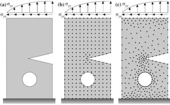
Figure 3.1 - a. Problem domain with the essential and natural boundaries applied. b. Regular nodal
discretization. c. Irregular nodal discretization.[40]
First, it is necessary to identify the outline of the solid problem, then is possible to define the natural and essential boundaries (Figure 3.1). After these two requirements are met, it is possible to discretize the domain problem using a nodal set (regular or irregular). An irregular mesh has low accuracy in the regions with low nodal concentration, but is possible to overcome this problem adding more nodes. The addition of new points does not increase the computational cost of the meshing task, since there is no pre-established relation between nodes (as the one existing in FEM).
After this step, the next one is to obtain the nodal connectivity. In FEM, there is a finite element mesh and the nodes that belong to the same element interact directly between themselves and the boundary nodes interact with boundary nodes of nearby elements. In meshless methods, the connectivity between nodes is given by the overlapping of influence-domains, when it comes to RPIM, and influence-cells, when it comes to NNRPIM.
The next step is to set the numerical integration scheme. So, it is required to construct a background integration mesh which can be nodal dependent or independent, the later having a higher accuracy. To have more accurate results with nodal dependent meshes, a stabilization
9
method is required but this increases the computational time. Next, it is possible to obtain the field variables under study by using approximation or interpolation shape functions. Both methods studied in this work use interpolation shape functions, with radial basis functions (RBF) with polynomial basis functions combined.
3.2.2. RPIM Formulation
3.2.2.1-
Influence-domains and nodal connectivity
The first step is to perform an initial nodal discretization of the problem domain, and then ensure the nodal connectivity between each node. First, areas or volumes are defined, depending if the problem is 2D or 3D, with a certain number of nodes.
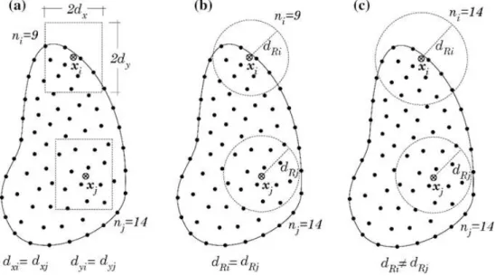
Figure 3.2 – a. Fixed rectangular shaped domain. b. Fixed circular shaped
influence-domain. c. Flexible circular shaped influence-domain [40]
As shown in Figure 3.2, influence-domains can have a fixed or variable size, however the latter is recommended since, fixed sized influence domains can lead to an uneven number of nodes inside the influence-domain of different nodes, which reduces the accuracy of the results. The second assures that every node’s influence-domain contains the same number of nodes, allowing to have shape functions with the same degree of complexity.
3.2.2.2-
Numerical integration
The RPIM uses the Gauss-Legendre integration scheme. So, first a background mesh must be created. This mesh can be created by the connection of the nodes discretizing the problem domain or a mesh larger than the problem domain. If the background integration mesh is larger than the problem domain, the points that are outside of the problem domain must be removed from the computation. The meshes can be quadrilateral or triangular.
10 Numerical methods
10
Inside of each one is possible to distribute the integration points, as shown in Figure 3.3.
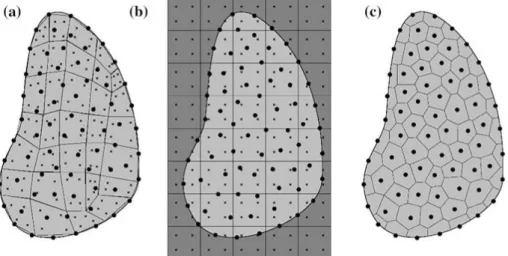
Figure 3.3 - a. Fitted Gaussian integration mesh. b. General Gaussian integration mesh. c. Voronoï
diagram for nodal integration [40]
Afterwards, it is used the Gauss-Legendre quadrature technique to obtain the background integration mesh (see Figure 3.4).
Figure 3.4 – a. Initial quadrilateral from the grid-cell. b. Transformation of the initial quadrilateral into
an isoparametric square shape and application of the 2 x 2 quadrature point rule. c Return to the initial quadrilateral shape [40]
First, the isoparametric weights and coordinates of each integration point are defined. Afterwards, the Cartesian coordinates of the integrated points are calculated using isometric interpolation functions.
where m represents the number of nodes in the element, and 𝑥𝑖 and 𝑦𝑖 represent the
Cartesian coordinates of the cell nodes. 𝑥 = ∑ 𝑁𝑖 𝑚 𝑖=1 (𝜉, 𝜂). 𝑥𝑖 𝑦 = ∑ 𝑁𝑖 𝑚 𝑖=1 (𝜉, 𝜂). 𝑦𝑖 (3.1)
11 For the quadrilateral integration cells:
For triangular integration cells:
The integration weight of the integration point is obtained by multiplying the isoparametric weight, of the integration point with the determinant of the Jacobian matrix of the respective cell.
Afterwards, the numerical integration is performed using,
where 𝜔𝑖 is the weight of the integration point 𝒙 in natural coordinates.
𝑁1 = 1 4
(
1 − 𝜉)(
1 − 𝜂)
; 𝑁2 = 1 4(
1 + 𝜉)(
1 − 𝜂)
; 𝑁3 = 1 4(
1 + 𝜉)(
1 + 𝜂)
; 𝑁4= 1 4(1 − 𝜉)(1 + 𝜂) (3.2) 𝑁1(
𝜉, 𝜂)
=1 −
𝜉 − 𝜂; 𝑁2(
𝜉, 𝜂)
= 𝜂; 𝑁3(
𝜉, 𝜂)
= 𝜉; (3.3) 𝐽 = [ 𝜕𝑥 𝜕𝜉 𝜕𝑦 𝜕𝜉 𝜕𝑥 𝜕𝜂 𝜕𝑦 𝜕𝜂] (3.4) ∫ ∫ 𝑓(𝜉, 𝜂)𝑑𝜉𝑑𝜂 = ∑ ∑ 𝜔𝑖𝜔𝑗 𝑛 𝑗=1 𝑓(𝜉, 𝜂) 𝑚 𝑖=1 1 −1 1 −1 (3.5)12 Numerical methods
12
4.2.3- NNRPIM Formulation
3.2.3.1-
Natural neighbours
This method uses the natural neighbour concept to determine the nodal connectivity, to obtain influence-cells. The natural neighbour geometric construction is based on the Voronoï diagram of the nodal distribution, from which it can be obtained the geometric and spatial relations between Voronoï cells.
The Voronoï diagram is a partition of the domain composed of 𝑁 closed and convex sub-regions (Voronoï cells), being 𝑁 the number of nodes in the discretization mesh, in which, each partition is associated with the node i in a way that any point in the interior of 𝑉𝑖 is closer to
𝑛𝑖 than to any other node 𝑛𝑗
Considering a set of 𝑵 distinct nodes, discretizing a certain space domain Ω ∈ ℝ2,
The Figure 3.5 shows the construction of a Voronoï cell of an interest node 𝑛0.
Figure 3.5 – a. Initial nodal set of potential neighbour nodes of node 𝑛0. b. First trial plane. c. Second
trial plane. d. Final trial cell containing just the natural neighbours of node 𝑛0. e. Node 𝑛0 Voronoï cell
𝑉0. f. Voronoï diagram [40]
13
A Voronoï cell is obtained for each node in the mesh and is defined as the geometric place for which all belonging points are closer to that node than to any other. The process to achieve a Voronoï cell is shown in Figure 3.5.
Using figure 3.5 and 𝑛0 as an example, it is possible to obtain a provisional Voronoï cell,
which contains all the neighbour’s nodes of 𝑛0. Nodes located outside the ones contained in
the provisional Voronoï cell are discarded. First, a potential neighbour must be chosen, for example 𝑛3 and determining vector 𝑢30,
Being 𝑢50= {𝑢30, 𝑣30, 𝑤30}. All nodes that follow this relationship,
are discarded.
Now, obtained the provisional Voronoï cell for node 𝑛0, it is possible to obtain the Voronoï
cell, 𝑉0. As shown in Figure 3.5, the distance between node 𝑛0 and the boundary of Voronoï
cell, 𝑉0 is half the Euclidian norm of node 𝑛0 and the neighbour node in question.
Using n3 as example, the distance between 𝑛0 and the boundary referring to node 𝑛3 is
given by,
Then, following the same reasoning for each node, it is possible to obtain the Voronoï diagram.
3.2.3.2-
Influence cells and nodal connectivity determination
In NNRPIM the nodal connectivity is imposed using the information coming from the Voronoï diagram. There are two types of influence-cells, accordingly to their level of nodal connectivity, as shown in Figure 3.6. The first-degree influence-cell of a point of interest consists of its natural neighbours (directly obtained by the Voronoï diagram). Concerning the second-degree influence-cell of a point of interest, it consists of the first natural neighbours considered in the first-degree influence-cell added to their own natural neighbours.𝑢30= (𝑥0− 𝑥3) ‖𝑥0− 𝑥3‖ (3.7) 𝑢30𝑥 + 𝑣30𝑦 + 𝑤30𝑧 ≥ (𝑢30𝑥3+ 𝑢30𝑦3+ 𝑤30𝑧3) (3.8) 𝑑𝑛0𝑛3= 𝐸(𝑥0, 𝑥3) 2 (3.9)
14 Numerical methods
14
Figure 3.6 - a. First degree influence-cell b. Second degree influence-cell [40]
3.2.3.3-
Numerical integration
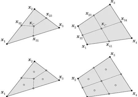
After constructing the Voronoï diagram, it is possible to obtain a nodal dependent integration mesh based on the nodal distribution special information. Primarily, the Voronoï cells are divided in sub-cells by the lines intersecting the central node and each neighbourhood node. For a regular mesh, the partition results are triangles and for irregular meshes the result are quadrilaterals.
Using the Delaunay tessellation (see Figure 3.7), the nodes of Voronoï cells sharing common boundaries are connected, and the overlap of both the Delaunay tessellation and the influence-cell boundaries leads to a smaller sub-influence-cell.
Figure 3.7 – a. Voronoï diagram, b. Delaunay triangulation and c. Natural neighbour circumcircles
[40]
Thus, the cell is divided in several sub-cells (in equal to number of neighbour nodes of its central node), being that its area, 𝐴𝑣, is equivalent to the sum of the areas of the sub-cells, 𝐴𝑆𝐼𝑖,
given by
Based on the Gauss-Legendre numerical integration numerical integration, integration points are inserted in the barycentre of each sub-cell (Figure 3.8).
𝐴𝑉𝐼= ∑ 𝐴𝑆𝐼𝑖
𝑛 𝑖=1
15
Figure 3.8 - Triangular shape and quadrilateral shape and the respective integration points 𝑥𝐼 using the Gauss-Legendre integration scheme [40]
This is an example for 1 integration point for each sub-cell. To use more integration points, each sub-cell is divided again into small quadrilateral sub-cells and the process is equal to the RPIM using quadrilateral cells. This process is repeated to all the other Voronoï cells, to obtain the domain integration.
3.2.3.4-
Shape functions
Both numerical methods presented in this work use the same methodology to construct the shape functions, using a combination of radial basis functions with polynomial functions.
Consider a function 𝑢(𝒙), defined in a certain influence-domain, discretizing by a set of N distinct nodes,
which can be rewritten as,
where 𝑅𝑖(𝒙𝐼) is the RBF, 𝑝𝑗(𝒙𝐼) is the polynomial basis function, 𝑛 is the number of nodes inside
the influence-domain of the interest point 𝒙𝐼 and 𝑎𝑖(𝑥𝐼) and 𝑏𝑗(𝒙𝐼) are non-constant coefficients
of 𝑅𝑖(𝒙𝐼) and 𝑝𝑗(𝒙𝐼) respectively. 𝑢(𝒙𝐼) = ∑ 𝑅𝑖(𝒙𝐼)𝑎𝑖(𝒙𝐼) 𝑛 𝑖=1 + ∑ 𝑝𝑗(𝒙𝐼)𝑏𝑗(𝒙𝐼) 𝑚 𝑗=1 = 𝑹𝑇(𝒙 𝐼)𝒂 + 𝒑𝑇(𝒙𝐼)𝒃 (3.11) 𝑢(𝒙𝐼) = ∑ 𝑅𝑖(𝒙𝐼)𝑎𝑖(𝒙𝐼) 𝑛 𝑖=1 + ∑ 𝑝𝑗(𝒙𝐼)𝑏𝑗(𝒙𝐼) 𝑚 𝑗=1 = {𝑹𝑇(𝒙 𝐼), 𝒑𝑇(𝒙𝐼)} { 𝒂 𝒃} (3.12) 𝑎𝑇(𝒙 𝐼) = [𝑎1(𝑥𝐼), 𝑎2(𝑥𝐼), … , 𝑎𝑛(𝑥𝐼) ] (3.13)
16 Numerical methods
16
This method uses the Multiquadric (MQ) function presented obtaining a MQ-RBF:
where c and p are two parameters whose optimal values were found as 0,0001 and 1,0001 [41], respectively, and 𝑟𝑖𝑗 the Euclidian norm between the integration point 𝒙𝐼 and a certain node
𝒙𝑖,
The polynomial basis are for 2D problems are:
To assure a unique approximation, the polynomial term must follow the rule:
The function can be reformulated to
Solving equation 2.24,
Substituting equation 3.25 in eq. 3.11, the shape function is obtained: 𝑏𝑇(𝒙 𝐼) = [𝑏1(𝑥𝐼), 𝑏2(𝑥𝐼), … , 𝑏𝑛(𝑥𝐼) ] (3.14) 𝑅𝑇(𝒙 𝐼) = [𝑅1(𝑥𝐼), 𝑅2(𝑥𝐼), … , 𝑅𝑛(𝑥𝐼) ] (3.15) 𝑝𝑇(𝒙 𝐼) = [𝑝1(𝑥𝐼), 𝑝2(𝑥𝐼), … , 𝑝𝑛(𝑥𝐼) ] (3.16) 𝑅𝑖𝑗 = (𝑟𝑖𝑗2+ 𝑐2)𝑝 (3.17) 𝑟𝑖𝑗 = √(𝑥𝑖− 𝑥𝐼)2+ (𝑦𝑖− 𝑦𝐼)2 (3.18) 𝑁𝑢𝑙𝑙 𝑏𝑎𝑠𝑖𝑠 − 𝒙𝑇 = {𝑥, 𝑦}; 𝑝𝑇(𝒙) = {0}; 𝑚 = 0 (3.19) 𝐶𝑜𝑛𝑠𝑡𝑎𝑛𝑡 𝑏𝑎𝑠𝑖𝑠 − 𝒙𝑇 = {𝑥, 𝑦}; 𝑝𝑇(𝒙) = {1}; 𝑚 = 1 (3.20) 𝐿𝑖𝑛𝑒𝑎𝑟 𝑏𝑎𝑠𝑖𝑠 − 𝒙𝑇 = {𝑥, 𝑦}; 𝑝𝑇(𝒙) = {1, 𝑥, 𝑦}; 𝑚 = 3 (3.21) 𝑄𝑢𝑎𝑑𝑟𝑎𝑡𝑖𝑐 𝑏𝑎𝑠𝑖𝑠 − 𝒙𝑇 = {𝑥, 𝑦}; 𝑝𝑇(𝒙) = {1, 𝑥, 𝑦, 𝑥2, 𝑥𝑦, 𝑦2}; 𝑚 = 6 (3.22) ∑ 𝑝𝑗(𝒙𝑖)𝑎𝑖= 0, 𝑗 = 1, 2, … , 𝑚 𝑛 𝑖=1 (3.23) [𝑹 𝒑 𝒑𝑻 𝟎] { 𝒂 𝒃} = { 𝒖𝒔 𝟎} = 𝑮 { 𝒂 𝒃} (3.24) {𝒂𝒃} = 𝑮−1{𝒖𝟎𝒔} (3.25)
17 which 𝜑(𝒙𝐼) is the shape function defined by
Since they respect the Kronecker delta property,
which means they pass through every single node within the domain (or influence-cell), in opposition to approximation shape functions which do not.
3.3 - Discretized formulation flow
In this section, it will be explained the flow formulation for viscoplastic materials. This deduction was extracted from Zienkiewicz et al. [42]. The problem variables are 𝒖, the velocity, 𝜺̇, the rate of strain defined by the operator S as
Being 𝑺 matrix is defined by
Where 𝜑 is the shape function and n is the number of nodes of the element in study that have the integration point 𝒙𝐼 or the number of nodes inside the influence domain of the
integration point 𝒙𝐼. The 𝒖 vector is defined by 𝒖 = {𝑢𝑥 𝑢𝑦} 𝑇
. As the “pressure” p is equal to the mean stress, the constitutive law defines stress as
where 𝜇 is the viscosity, 𝝈 is the stress, 𝛿𝑖𝑗 is the delta Kronecker and 𝑫0 and m are matrices
avoiding the need for tensorial notation. Notice that it can be verified that the matrix 𝑫0 has
the following form:
𝑢(𝒙𝐼) = {𝑹𝑇(𝒙𝐼), 𝒑𝑇(𝒙𝐼)}𝑮−1{ 𝒖𝑠 𝟎} = 𝜑(𝒙𝐼)𝒖𝑠 (3.26) 𝜑(𝒙𝐼) = {𝑹𝑇(𝒙𝐼), 𝒑𝑇(𝒙𝐼)}𝑮−1= [𝜑1(𝒙𝐼), 𝜑2(𝒙𝐼), … 𝜑𝑛(𝒙𝐼) ] (3.27) 𝜑(𝒙𝑗) = { 1, 𝑖 = 𝑗, 𝑗 = 1, 2, … , 𝑛 0, 𝑖 = 𝑗, 𝑗 = 1, 2, … , 𝑛 (3.28) 𝜺̇ = 𝑺𝒖 (𝑜𝑟 𝜀̇𝑖𝑗= 𝑢𝑖,𝑗+ 𝑢𝑗,𝑖 2 ) (3.29) [𝑺]𝑰= [ 𝑑𝜑1 𝑑𝑥 0 0 𝑑𝜑1 𝑑𝑦 𝑑𝜑1 𝑑𝑦 𝑑𝜑1 𝑑𝑥 | | … | | 𝑑𝜑𝑛 𝑑𝑥 0 0 𝑑𝜑𝑛 𝑑𝑦 𝑑𝜑𝑛 𝑑𝑦 𝑑𝜑𝑛 𝑑𝑥 ] (3.30) 𝜎 = 𝜇𝑫0𝜀̇ + 𝒎𝑝 (𝑜𝑟 𝜎𝑖𝑗 = 2𝜇 (𝜀̇𝑖𝑗− 𝛿𝑖𝑗𝜀𝑘𝑘 3 ) + 𝛿𝑖𝑗𝑝) (3.31)
18 Numerical methods 18 𝑫0 = [ 4 3 − 2 3 − 2 3 0 0 0 −2 3 4 3 − 2 3 0 0 0 −2 3 − 2 3 4 3 0 0 0 0 0 0 1 0 0 0 0 0 0 1 0 0 0 0 0 0 1] (3.32)
Although the inverse of 𝑫0 does not exist, the inverse relation can be written as,
With
And 𝒎 = {1 1 0} for a 2D problem. In general 𝜇 is dependent from the stain rate and the total accumulated strain, so the system is non-linear. For many viscoplastic materials the viscosity follows this relation:
Where 𝜎𝑦 is the uniaxial yiels stress which, for strain hardening, is a function of the
accumulated second strain invariant 𝜀̃ and temperature T. 𝛾 is the fluidity parameter
and 𝜀̃ is the second invariant of the strain rate
Assuming pure elasticity, 𝛾 is considered null: 𝛾 = 0.
The governing equations of the problem are now momentum conservation (with 𝜎 defined by equations 3.8 and 3.9 and b the body force).
where S is the strain operator, pointed in equation 3.7, and incompressibility 𝜺̇ =1 𝜇𝑫 −1(𝝈 − 𝒎𝑝) (3.33) 𝑫−1= [ 2 0 0 0 0 0 0 2 0 0 0 0 0 0 2 0 0 0 0 0 0 1 0 0 0 0 0 0 1 0 0 0 0 0 0 1] (3.34) 𝜇 = (𝜎𝑦+ 𝛾𝜀̃̇𝑚)/3𝜀̃̇ (3.35) 𝜎𝑦= 𝜎𝑦(𝜀,̃ 𝑇) (3.36) 𝜀̃̇ = (2 3𝜀̇𝑖𝑗∙ 𝜀̇𝑖𝑗) 1 2⁄ (3.37) 𝑺𝑇𝝈 + 𝒃 = 0 (𝑜𝑟 𝜎 𝑖𝑗,𝑖+ 𝑏𝑖= 0) (3.38) 𝒎𝑇𝑺𝒖 = 0 (or 𝑑𝑢 𝑑𝑥+ 𝑑𝑣 𝑑𝑦= 0) (3.39)
19
In the problem domain Ω with the right boundary conditions on tractions (on Γt) or velocities (on Γu). The standard Galerkin discretization process with
where 𝑵𝒖 is the shape functions of velocity and 𝑵𝑝 are the shape functions of pressure:
Notice that the shape functions for the velocities are obtained in the integration points, considering the full integration mesh, and the shape functions for pressures are obtained in the reduced integration mesh (considering the integration point coincident with the nodes). This leads to
in which
where K is the stiffness matrix, Q is matrix imposing the incompressible condition and f is the force. In the preceding discretization it is necessary to assure that the resulting equations are never singular so that convergence is assured by the Babuska-Brezzi condition.
where I is the identity matrix and 𝛼 the penalty number taken as 𝛼 = 107𝜇. This results in a
single matrix element stiffness matrix
and the final assembled non-linear system of equations
𝒖 ≈ 𝒖̂ = 𝑵𝑢𝒖 𝑎𝑛𝑑 𝑝 = 𝑵𝑝𝒑̅ (3.40) 𝑵∗= [ 𝜑1∗ 0 0 𝜑1∗| … | 𝜑𝑛∗ 0 0 𝜑𝑛∗] (3.41) [𝑲 𝑸 𝑸𝑻 𝟎] [ 𝒖 ̅ 𝒑] = [ 𝒇 𝟎] (3.42) 𝑲 = ∫ ( 𝑺𝑵𝑢)𝑇𝜇𝑫𝟎 Ω (𝑺𝑵𝑢) 𝑑Ω (3.43) 𝑸 = ∫ (𝑺𝑵𝑢)𝑇 Ω 𝒎𝑵𝑝𝑑Ω (3.44) 𝒇 = ∫ 𝑵𝑢𝑇𝒃𝑑Ω + Ω ∫ 𝑵𝑢𝑇𝒕𝑑Γ Γt (3.45) [𝑲𝒆 𝑸𝒆 𝑸𝒆𝑻 𝑰⁄𝛼 ] [𝒖𝒆 𝑷𝒆 ] = [𝒇𝒆 𝟎] (3.46) 𝑲𝑒𝒖𝑒= (𝑲𝑒− 𝑸𝑒𝑸𝑒𝑇)𝒖𝑒= 𝒇𝑒 (3.47) 𝑲𝒖 = 𝒇 (3.48) 𝑲 = 𝑲(𝒖), 𝜇(𝜺̇) = 𝜇(𝒖) (3.49)
20 Numerical methods
20 Which is solved iteratively
3.4 - Numerical analysis applied to blood flow
The blood flow studies are in arteries, such as hemodynamics of bypass graft for stenosed arteries, hemodynamics of stented aneurysm at the aortic arch and hemodynamics of bypass treatment for DeBakey III aortic dissection. [1]
The main methods to simulate blood flow in this vessel are one-dimensional Navier-Stokes finite element model for elastic networks and the Hagen-Poiseuille model for rigid networks. These models are Newtonian, but the second can be used like a Poiseuille-like non-Newtonian flow through the inclusion of time-independent non-Newtonian effects using a vessel-dependent non-Newtonian effective, which is computed and updated iteratively to reach a consistent flow solution over the whole network. [19]
Using meshless methods in blood flow analysis is still unusual; The most used methods are Smooth Particle Hydrodynamis (SPH) and localized meshless method (LCMM).[38], [43]
In order to simulate the blood flow with the three methods descripted before (FEM, RPIM and NNRPIM), it was necessary to use a software that could run those formulations.
FEMAS is a Finite Element and Meshless Analysis Software fully developed by Prof. Dr. Jorge Belinha. FEMAS possesses a graphical user interface (GUI) running in Matlab environment (see Figure 3.9). This software allows to analyse a model with FEM, RPIM and NNRPIM.
Other functionality of this software is to design 2D and 3D models. It is possible to select the material proprieties and perform geometrical transformations on the models.
It permits to study structural problems considering 3D approaches, assuming one of the following analysis:
Linear Elasto-static analysis
Free Vibration linear elastic analysis
Buckling linear elastic analysis
Elasto-plastic non-linear analysis
Bone tissue remodelling analysis
Fluid flow analysis (low velocities)
It allows to use Finite element method (2D triangular elements with 3, 4 and 6 nodes and 2D quadrangular elements with 4, 8 and 9 nodes, and 3D tetrahedral elements with 4, 8 and 10 nodes and 3D hexahedral elements with 9, 20 and 27 nodes) and meshless methods (2D and 3D). To design more complex models, it was used a finite element mesh generator commercial code.
21
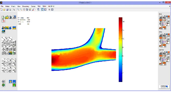
Figure 3.9 – Finite Element and Meshless Analysis Software (FEMAS) - Print-screen of an artery
22 Numerical methods
Chapter 4
Preliminary studies
In every new technique applied to a specific field, it is important to study its limitations and its advantages. Since there is not previous studies with the meshless methods described earlier, it is important to perform a thorough study in several geometries.
This chapter presents studies in 2D and 3D and aims to compare FEM with NNRPIM and RPIM. In this chapter, all the figures have the maximum and minimum velocity explicated, to help reading the colour scale.
4.1- 2D convergence studies
The work in this chapter aims to compare each numerical method and determine which level of discretization is necessary to have the most accurate results in different geometries. In this convergence study, there were build 6 different models with different geometries, each with different 4 meshes. These were successively refined following a rule on 2n. For each mesh, there were made 4 analysis: FEM with 2D triangular elements with 3 nodes and another with triangular elements with 6 nodes, RPIM and NNRPIM. The models were built using FEMAS.
Another goal of this convergence study is to evaluate the maintenance of the discharge though the model. Assuming that there is mass conservation, the discharge should be constant throughout the model. The last goal is to compare the different velocity profile in sections of the model.
In these simulations, blood was simulated as a Newtonian isotropic fluid. The viscosity is 3,5x10-06 N.ms/mm2 and the density is 1,05 kg/mm3.
Before running an analysis, it is necessary to define the boundary conditions (natural and essential). To assess the best boundary conditions preliminary tests were performed: it was tested a normal boundary condition (for all nodes in the boundary walls it was allowed displacements along the wall line/surface) and a fully clamped boundary condition (all nodes in the boundary walls were constrained both in x and y direction).
24 Preliminary studies
24
It was verified that the first condition was not suited for models with some degree of curvature (the velocity in the walls was different from 0). Therefore, all models used in convergence tests used the second condition. With this technique, the fluid is unable to pass beyond the artery’s walls. Moreover, in end of the vessel, no boundary conditions were applied, allowing the fluid to freely exit the domain.
At the entry, it was applied a velocity profile. The velocity profile of a fluid in laminar regime is described by a parabolic equation, as shown in Figure 4.1.
The equation of a parabola can be generically written as:
Assuming the velocity profile in the walls is 0 and H/2 is maximum:
It is possible to obtain the non-constant parameters of the parabolic expression:
The values for the maximum velocity in the convergence tests is 0.15 mm/ms.[46] This value was based on the maximum velocity in veins and the height is based on a credible diameter for a deep vein of the pelvis.
Figure 4.1 – Laminar velocity profile in a tube [45]
𝑢(𝑟) = 𝑎(𝑟)2+ 𝑏𝑟 + 𝑐 (4.1) { 𝑎(𝐻)2+ 𝑏𝐻 + 𝑐 = 0 𝑎(0)2+ 𝑏 × 0 = 0 𝑎(𝐻 2⁄ )2 + 𝑏 × 𝐻 2⁄ = 𝑉𝑚𝑎𝑥 (4.2) { 𝑎 =−4𝑉𝑚𝑎𝑥 ℎ2 𝑏 =4𝑉𝑚𝑎𝑥 ℎ 𝑐 = 0 (4.3)
25
The Figure 4.2 shows how the boundary conditions are represented in FEMAS.
Figure 4.2 – Example of the boundary conditions applied
As presented in previous sections, the performance of the NNRPIM and RPIM formulation depends on some parameters, such as the size of the influence domain, the MQ-RBF shape parameters, the polynomial basis and the integration scheme.
The parameters presented in Table 4.1, are the standard values used in the analysis. In some models and meshes, these parameters had to be adjusted to have more accurate results. These changes will be mentioned in the examples that didn’t used the parameters in Table 4.1.
Table 4.1 – Default RPIM and NNPIM used in the analysis
RPIM NNRPIM Influence domain Number of nodes inside the influence domain 16 Influence
cells Order Second
RPI shape functions Parameter c 1.42 RPI shape functions Parameter c 0.0001 Parameter p 1.03 Parameter p 0.9999
Polynomial Constant Polynomial Constant
Integration scheme Gauss points 1 Integration scheme Integration 1 (full integration)
The quantitative comparison between the three techniques is the most suited comparison methodology. Thus, three types of charts were created:
The discharge in each cross section on a given model with a certain discretization level, for each numerical method;
The discharge for each discretization level on a given cross section, for each numerical method;
26 Preliminary studies
26
The velocity profile in a given cross section
As mentioned before, the discharge must be constant. Thus, after obtaining the velocity for each node, this variable was calculated, as follows:
Where 𝑄𝑒 is the discharge, 𝑣𝑒𝑖 is the velocity in each node of the cut and 𝐴𝑒𝑖 area occupied
by the node.
In order to calculate the area that each node represents, the next methodology was followed. Considering that Figure 4.3 represents the area occupied by each node, it is perceptible that the area is calculated differently for the nodes in the border and nodes in the middle.
Figure 4.3- Representation of the nodes in a cross section
Assuming the thickness of the model is 1 mm, the area of the lateral nodes and the interior nodes is respectively
where 𝑛 is the number of nodes in the cross section. Theoretically, the result should be the integration of the velocity profile. The comparison is always made between models with the same number of nodes, rather than the same number of elements.
4.1.1-
Linear model
The Figure 4.4 presents the first model. The meshes (a), (b), (c) and (d) with triangular elements with 3 nodes have, respectively, 21, 65, 255 and 833 elements. The same meshes with triangular elements with 6 nodes have, respectively, 65, 225, 833 and 3201 nodes.
The model has 30 mm of length and 10 mm of height. Following equation 7.3, the initial velocity profile is:
𝑄𝑒= ∑ 𝑣𝑒𝑖 𝑁 𝑖 𝐴𝑒𝑖 (4.4) 𝐴𝑒𝑖 = 𝐷 2(𝑛 − 1) 𝐴𝑖𝑒= 𝐷 𝑛 − 1 (4.5)
27 and therefore, the theoretical discharge should be:
Figure 4.4 – Linear model with different meshes
a. 24 elements b. 96 elements c. 384 elements d. 1536 elements
𝑢(𝑟) = 0.06(𝑟)2− 0.006𝑟 (4.6)
(4.7)
(a) (b)
28 Preliminary studies
28
4.2.3- Results
The velocity maps are presented in the Figure 4.5, Figure 4.6, Figure 4.7, Figure 4.8 and Figure 4.9.
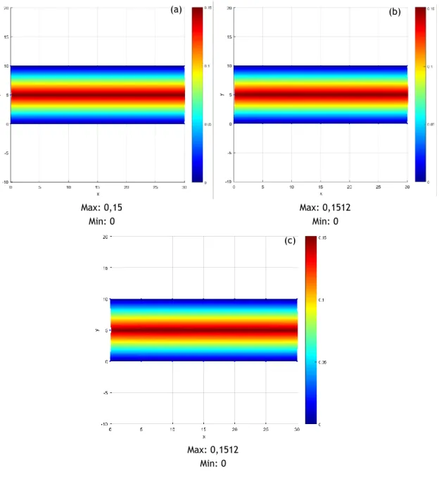
Figure 4.5 represents the analysis of the linear model with 21 nodes.
Max: 0,15 Min: 0 Max: 0,1512 Min: 0 Max: 0,1512 Min: 0
Figure 4.5 – Linear model (21 nodes) analysed with different methods a. FEM (triangular elements with 3 nodes) b. NNRPIM c. RPIM
In Figure 4.5, the results are similar between FEM with triangular elements with 3 nodes, NNRPIM and RPIM, with the same maximum velocity.
Figure 4.6 represents the analysis of the linear model with 65 nodes.
(a) (b)
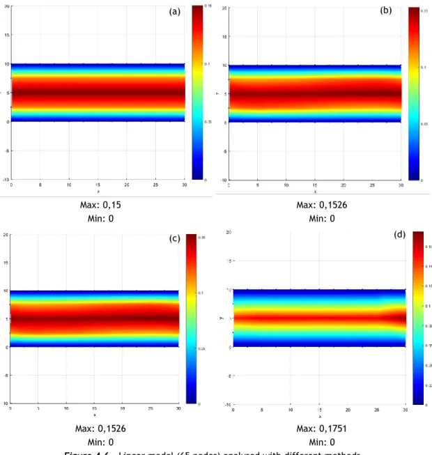
29 Max: 0,15 Min: 0 Max: 0,1526 Min: 0 Max: 0,1526 Min: 0 Max: 0,1751 Min: 0
Figure 4.6 – Linear model (65 nodes) analysed with different methods
a. FEM (triangular elements with 3 nodes) b. NNRPIM c. RPIM d. FEM (triangular elements with 6
nodes)
In Figure 4.6, the results are similar, with NNRPIM and RPIM with a slightly higher velocity. The FEM with 6 nodes per element, the maximum velocity is higher (above 0,16 mm/mms) and the velocity increases in the end of the model.
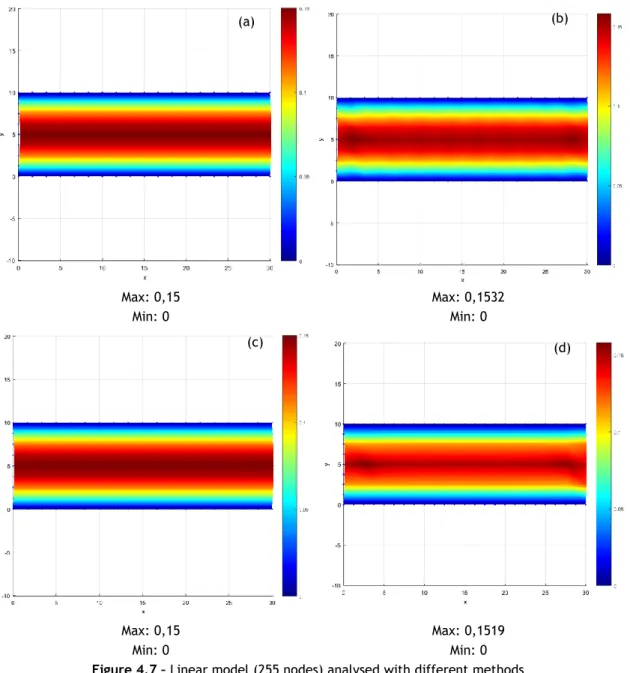
Figure 4.7 represents the analysis of the linear model with 65 nodes.
(a) (b)
![Figure 2.1 - Human blood viscosity as a function of shear rate for a range of hemaocrit concentrations on a log-log plot [21][22][23][19]](https://thumb-eu.123doks.com/thumbv2/123dok_br/15708812.1068589/30.892.199.703.116.484/figure-human-blood-viscosity-function-shear-hemaocrit-concentrations.webp)