Automated ICD-9-CM medical coding of diabetic patient’s clinical reports

(1)

Universidade de Aveiro Departamento deElectrónica, Telecomunicações e Informática 2018

Vitor Manuel de

Sousa Pereira

Codificação médica ICD-9-CM automatizada de

relatórios clínicos de pacientes diabéticos

Automated ICD-9-CM medical coding of diabetic

patient’s clinical reports

(2)

(3)

Universidade de Aveiro Departamento deElectrónica, Telecomunicações e Informática 2018

Vitor Manuel de

Sousa Pereira

Codificação médica ICD-9-CM automatizada de

relatórios clínicos de pacientes diabéticos

Automated ICD-9-CM medical coding of diabetic

patient’s clinical reports

Dissertação apresentada à Universidade de Aveiro para cumprimento dos requisitos necessários à obtenção do grau de Mestre em Engenharia de Com-putadores e Telemática, realizada sob a orientação científica do Doutor José Luís Guimarães Oliveira, Professor Associado do Departamento de Elec-trónica, Telecomunicações e Informática da Universidade de Aveiro e do Doutor Sérgio Guilherme Aleixo de Matos, Professor Auxiliar do Departa-mento de Electrónica, Telecomunicações e Informática da Universidade de Aveiro

(4)

(5)

o júri / the jury

presidente / president Doutora Ana Maria Perfeito Tomé Professora Associada, Universidade de Aveiro vogais / examiners committee Doutor Joel Perdiz Arrais

Professor Auxiliar, Faculdade de Ciências e Tecnologia da Universidade de Coimbra

Doutor Sérgio Guilherme Aleixo de Matos Professor Auxiliar, Universidade de Aveiro

(6)

(7)

agradecimentos / acknowledgements

(8)

(9)

Resumo A atribuição de códigos ICD-9-CM a relatórios clínicos de pacientes é um processo dispendioso e cansativo, realizado por pessoal médico especializado e com um custo estimado de 25 mil milhões de dólares por ano nos Esta-dos UniEsta-dos. É uma constante ambição de investigadores desenvolver um sistema que automatize esta atribuição. No entanto, o problema mantém-se irresoluto dadas as dificuldades inerentes em processar texto clínico não estruturado.

Este problem é aqui formulado como um de aprendizagem supervisionada

multi-label em que a variável independente é o texto do relatório e a

depen-dente os vários códigos ICD-9-CM atribuídos. São investigadas diferentes variações de dois modelos baseados em redes neurais, o Bag-of-Tricks e a Rede Neural Convolucional (RNC). Os modelos são treinados no subcon-junto de pacientes diabéticos dos dados MIMIC-III.

Os resultados mostram que uma RNC com três níveis convolucionais em paralelo obtém avaliações F1 de 44.51% para códigos de cinco dígitos e 51.73% para códigos abreviados de três dígitos. Além disto, é mostrado que a combinação de vários classificadores binários num só, com o método de relevância binária, produz uma melhoria de 7% em relação ao seu equiv-alente multi-label, num problema de classificação limitado aos onze códigos mais comuns nos dados.

(10)

(11)

Abstract The assignment of ICD-9-CM codes to patient’s clinical reports is a costly and wearing process manually done by medical personnel, estimated to cost about $25 billion per year in the United States. To develop a system that automates this process has been an ambition of researchers but is still an unsolved problem due to the inherent difficulties in processing unstructured clinical text.

This problem is here formulated as a multi-label supervised learning one where the independent variable is the report’s text and the dependent the several assigned ICD-9-CM labels. Different variations of two neural network based models, the Bag-of-Tricks and the Convolutional Neural Network (CNN) are investigated. The models are trained on the diabetic patient subset of the freely available MIMIC-III dataset.

The results show that a CNN with three parallel convolutional layers achieves

F1 scores of 44.51% for five digit codes and 51.73% for three digit, rolled up, codes. Additionally, it is shown that joining several binary classifiers, with the binary relevance method, produces an improvement of almost 7% over its multi-labeling equivalent in a restricted classification task of only the eleven most common labels in the dataset.

(12)

(13)

List of Figures

2.1 Conceptual overviews of the steps taken by a text mining system . . . 6

2.2 A first-order chain-linear CRF . . . 10

2.3 A graph representation of a 3-layer feedforward densely connected neural network 12 2.4 A recurrent neural network . . . 12

2.5 Generic clustering example . . . 13

2.6 Dependency tree obtained using Google’s SyntaxNet . . . 15

3.1 Radiology report example . . . 20

3.2 ECG (Electrocardiography) report example . . . 20

3.3 Number of occurrences for standardly grouped ICD-9-CM codes on the MIMIC-III subset . . . 22

3.4 Report lengths in tokens for reports with sizes which range from 0 to 800 . . 23

3.5 Distribution of reports per category . . . 24

3.6 Baseline Bag-of-Tricks . . . 27

3.7 Convolutional Neural Network models . . . 29

3.8 Category augmented model architectures . . . 30

(16)

(17)

List of Tables

3.1 Preprocessed dataset description . . . 24

3.2 The eleven most common rolled up ICD-9-CM codes . . . 25

3.3 The eleven most common rolled up ICD-9-CM codes per category . . . 25

3.4 Results for the multi-label classification sub-task . . . 32

3.5 Results for the binary classification sub-task . . . 33

3.6 Multi-label vs. binary classifier results for the most common labels . . . 34

(18)

(19)

Acronyms

BoT Bag-of-Tricks

CNN Convolutional Neural Network CRF Conditional Random Fields EHR Electronic health record

ICD-9-CM International Classification of Diseases, 9th Version, Clinical Modification LSTM Long Short-Term Memory

MIMIC-III Medical Information Mart for Intensive Care III NER Named-Entity Recognition

PMI Pointwise Mutual Information POS Part-of-speech

RNN Recurrent Neural Network SVM Support Vector Machine

UMLS Unified Medical Language System

(20)

(21)

Chapter 1

Introduction

Over the past decade, significant advancements have been made in data production and collection, as well as in the development of analysis techniques to leverage all this information. Accumulating and processing these voluminous datasets — coined big data — is allowing every industry to make better informed, data-driven decisions. Health care is no exception. Medical data was estimated to be growing at the annual rate of 48% and is expected to reach an astonishing 2 314 exabytes by 2020 [1].

Trailing this growth of data, at a much less pronounced rate but nonetheless important, is the increase in national health expenditures. In Portugal, health expenditures have been increasing at least since 2016 [2]; in the United States, they reached 17.8% of the Gross Domestic Product in 2015 [3]. It is undoubtedly in the interest of governments and health institutions to invest in digital health and make the most out of their data, if for nothing else, to reduce costs. Most importantly, researchers have indicated that such digital health ventures, if successful, could prove to be immensely beneficial in enhancing the efficiency of care delivery, especially in regards to patient safety and quality [4, 5].

Increasingly, health data is generated by the patients themselves using devices like sensor enabled smartphones, at-home genetic testing kits and all sorts of wearables. It is, although, in electronic health records, produced by health professionals and generally written in free-flowing text where most information resides. Fully using these records, despite potential benefits, remains an underexplored topic mostly because of the unique challenges processing this type of data presents.

Electronic health records capture the state of a patient across time and are invaluable in diagnosis. Besides this, they play a significant part in the reimbursement process of health institutions by insurance companies. Medical codes, like ICD-9-CM, assigned to patient’s reports after treatment serve as a justification for carrying out the said treatment. Failure in correctly assigning these codes is a liability for healthcare institutions: a missing code represents a loss of revenue and an extra one can constitute fraud. Assigning and correcting these codes is done manually by specialized medical personnel, called a medical coders, and is estimated to cost about $25 billion per year in the United States [6].

It is the aim of this thesis to develop a system which automates the assignment of ICD-9-CM codes to clinical reports. This is achieved by developing a statistical classification model which approximates a function parameterizing the relation between a report’s textual contents and its assigned codes. The used classifiers are based on artificial neural networks, which have shown to be capable of handling large volumes of relatively messy data [7].

(22)

The classifier is developed on the diabetic patient subset of the MIMIC-III dataset. By constraining the system to this subset, its diseases, terminology and patterns, it is made less versatile but the lesser variability sets it up to produce more accurate results.

Chapter 2 explores the challenges in processing free-flowing clinical text and the methods researchers have developed to meet this challenge. Chapter 3 takes a close look at the MIMIC-III dataset and presents the used neural network models as well as their results. Chapter 4 briefly summarizes the accomplished and presents some suggestions for further work.

(23)

Chapter 2

Literature Review

This chapter will serve as an introduction to clinical text mining and its state-of-the-art techniques.

2.1 Text Mining

As the volume of data stored in electronic health records (EHR) keeps increasing, manual analysis of this data, done by professionals, to extract relevant information becomes a chal-lenging task. As such, a focus point for scientists and information technology professionals has been to develop methods which ease and automate this kind of analysis.

Text mining is the field of data mining which concerns itself with the extraction of valuable information from unstructured sources. This process mostly works by finding interesting patterns and trends in text.

2.1.1 Clinical Text

Most research in biomedical text mining focuses on extracting information from scientific literature. Two compelling reasons can justify this focus. First, large swathes of data, in the form of scientific articles, are available to researchers who have access to journals such as

Cell and Nature. Even more data is accessible to everyone through preprint archival projects

such as arXiv and bioRxiv. Second, authors aim for accurate, concise, clear and objective language in writing their articles [8]. This, together with the fact that they follow a predictable structure, — “Introduction”, “Prior Work”, “Methods”, “Results”, “Conclusion” — results in texts which are readier for mining.

Clinical text mining offers no such advantages. In the United States, hospitals host pa-tient’s health records in local servers running proprietary software from different providers that are largely incompatible, preventing institutions from exchanging patient data among themselves [9]. This makes large amounts of patient data inaccessible to medical practition-ers and researchpractition-ers alike. In Portugal, a state funded EHR manager, the “Registo de Saúde Electrónico”, was introduced in 2010 but is underutilized as public and private hospitals and clinics choose to keep running their already installed systems making the situation very much alike to that of the US [10].

Furthermore, patient EHR data is highly private so before being made available to re-searchers it needs to be anonymized by the institution that owns the data. Legislation like

(24)

the Health Insurance Portability and Accountability Act, in the US, and the General Data Protection Regulation, in the EU, regulate how the data is to be anonymized and make sure serious violations result in serious fines. In practice, this means that, even if data anonymiza-tion is automated, manual compliance checking, by legal professionals, is usually required. This is yet one more disicentive for institutions to make the data available.

The structure and content of clinical text is also not neatly defined like in scientific lit-erature. Meystre et al. sum up the challenges in mining clinical text when compared to biomedical scientific literature [11].

First, a single patient’s record has several types of report. These can be the patient’s description, his and his family’s medical history, remarks made by the physician during an examination, etc. The length of the reports also varies greatly e.g. writing a couple of vital signs during a routing check-up vs. the patient’s full medical history during the first consultation. Related to length is the structure of the reports. EHR software is usually form-based (“symptoms”, “suggested causes”, “suggested treatment”, …) which could result in thematically well defined short sentences for each of the form’s fields. However, the clinician might opt to ignore the form’s structure and use the free-form data entry field, if it is available, or, worst case, misuse one of the other form entries, if it is not, to introduce the report’s data. The clinician also appropriates his writing style and language depending on if the text is going to be read by other practitioners. A report, written by a radiologist, which accompanies an x-ray is composed for clear communication. In contrast, notes written by a physician during a consultation are not. These can be ungrammatical, ignoring capitalization and punctuation rules, and composed of short, telegraphic phrases where shorthand abounds — homonyms, acronyms, abbreviations and local dialectal shorthand phrases. Furthermore, the shorthand can be overloaded i.e. the same shorthand unit takes a different meaning depending on surrounding context. According to the 2015AA version of UMLS, the abbreviation “RA” can stand for 25 meanings as distant as “rheumatoid arthritis”, “radioactive” and “ragweed antigen” [12]. Liu et al. show that 33% of the time acronyms in UMLS are highly ambiguous even in context [13]. Lexical, morphological and spelling errors also proliferate in clinical text. Ruch and Gaudinat report that about up to one in every five sentences in a corpus of discharge summaries, surgical reports and laboratory results has a spelling error [14]. It is not uncommon to find the acronyms themselves misspelled [11]. Text can also be interrupted by values copy-pasted from laboratory results, vital signs or drug dosages which can confuse standard text mining algorithms like sentence segmentation.

All these characteristics make clinical text particularly challenging for information extrac-tion tasks.

2.1.2 Clinical Text in Portuguese

Text mining clinical text in Portuguese presents yet additional challenges. First and foremost, much less research work has been done in text mining in Portuguese than in English. Second, Portuguese is a morphologically very rich language. While nouns and adjectives have 4 forms (two genders, either masculine or feminine, and two numbers, either singular or plural), verbs have 66 different forms (two numbers, three persons and five modes each with a variable number of tenses) [15].

A recently instituted change added more variability to written Portuguese. The “Acordo Ortográfico da Língua Portuguesa de 1990” is an international treaty finalized in 1990, ratified by the Portuguese parliament in 2008 and its use made mandatory in 2015 which introduced

(25)

several orthographic changes into the Portuguese language. These changes can be summarized as such:

• Capitalization changes such as months and weekdays being written in lowercase and forms of address with optional capitalization (“doutor” vs. “Doutor”).

• Removal of “mute” consonants (i.e. when they are written but not pronounced). For example, “acção” becomes “ação”.

• Graphic accent usage. Words which were previously accentuated now are not. E.g. “pára” vs. “para” and “pêlo” vs. “pelo”.

• Significant changes in regards to the usage of the hyphen. Some words like “pára-quedas” lose the hyphen (and the graphic accent) and become “paraquedas”. With other words like “cor-de-rosa” and “cor de rosa” there does not seem to be a consensus1_.

The alterations to the language were not put into action without contest and several high profile dissenters [16]. The result of these changes is that some people choose to write according to the treaty, some choose to ignore it and some freely mix pre and post-treaty orthography.

Nevertheless, some pioneering researchers have done work in extracting information from clinical text written in Portuguese. Pereira uses EHR from children with epilepsy to develop a system which aids doctors in choosing the course of treatment by recommending medications and procedures [17]. Castro uses machine learning text mining techniques to classify patient’s allergy records according to SNOMED CT terminology [18]. Ferreira et al. develop MedInX, an information extraction system which accurately maps free text discharge reports onto a structured representation using natural language processing [19].

2.1.3 Overview of Text Mining

Figure 2.1 illustrates two variants of conceptual clinical text mining systems. Campos et al. offer in [20] a description of the illustrated steps.

Pre-processing is the first stage of the pipeline. The input unstructured text is split into sentences which are further split into meaningful units called tokens. The software which does this kind of processing is called a tokenizer. Choosing a good tokenization method is critical as all further processing will be executed on the tokens. An example used with biomedical information is SPECIALIST NLP2_.

Following this, there is a need to normalize the tokens, reducing them to a canonical form.

Stemming replaces inflected or derived words with their word stem — a form to which suffixes

can be attached. “Children”, “childish” and “childless” will be reduced to the stem form “child”. A more complex approach is lemmatization. Stemmers might output words which have no actual meaning. For example “argues” and “argument” become “argu”. Lemmatizers use part-of-speech information to find the token’s root form — its lemma. In the previous example, the lemma would be “argue”. POLARIS is a lexical database which can be used to generate lemmas for words in Portuguese [21].

In English, words like “the”, “be” “this”, “that”, etc. prove to be non-informative during further processing. Other languages have equivalent non-informative words. These can be

1_{https://ciberduvidas.iscte-iul.pt/consultorio/perguntas/acerca-de-cor-de-rosa-e-cor-de-laranja/29892} 2_{https://lexsrv3.nlm.nih.gov/Specialist/Home/index.html}

(26)

Relation Extraction

Post-Processing Named-Entity Recognition

Annotated Entities

Unstructured Text / Training Data

Pre-Processing

(a) Relation extraction pipeline.

Training Data Pre-Processing Post-Processing Classification Labels (b) Classification pipeline.

Figure 2.1: Conceptual overviews of the steps taken by a text mining system. They do not represent the actual data flow of an hypothetical implementation just the steps it might take.

(27)

discarded during a process called stopword removal where a pre-made list of these words is used.

The next step, named-entity recognition, is the basic building block for most informa-tion extracinforma-tion tasks. Here, biomedical entities deemed pertinent are identified and classified. These might be genes, chemicals, drugs and diseases. To do this, rule-based, dictionary-based and, more recently, machine learning-based methods are used. When the last are used, it might also be necessary to do feature engineering and the existence of a large corpus of pre-annotated training data. Alternatively, in a classification system, a statistical model is developed to assign each of the datum in the pre-annotated training corpus to a pre-defined category. A practical example is the automated assignment of UMLS codes to clinical reports. After the named-entities are identified, there is still the need to establish relations among them and other words in the sentence. This is done in the relation extraction phase. An invaluable tool in this step are syntactic parsers which output dependencies between all words in a sentence. This information can be combined with the entities obtained in the previous step and input into a machine learning model.

As these methods are not perfect, post-processing their results may be necessary. Un-informative, incorrect and unwanted annotations can be discarded. Correct annotations can be manually extended and be made more precise [22]. Labels need to be mapped to their actual value from whatever intermediate representation might have been used.

Named-entity recognition, relation extraction and classification are the main focus of this thesis and are discussed, at length, in following sections.

2.2 Named-Entity Recognition

Named-entity recognition (NER) in the biomedical domain is considered particularly chal-lenging compared to other domains due to inconsistencies in entity naming. A certain drug can be referred to by its chemical name, generic name, brand name, a standard or nonstandard abbreviation.

NER can be said to be a two step task: term extraction and term classification. In term extraction, terms which might be of interest in text are determined, in term classification, a label is attributed to these terms.

Most recent work in biomedical NER focuses on the genetics subdomain. These tools focus on extracting proteins, genes and mutations from text. Systems such as BANNER [23] and BABELOMICS [24] focus on gene extraction while tmVar [25] takes a step further and focuses on gene mutations. This interest can possibly be explained by the usefulness of this kind of tool in oncology [26].

Following the trend in general NER, biomedical NER systems have evolved from hand-crafted rule-based systems, to dictionary-based, to machine learning-based ones [22, 27]. Handcrafted rule-based systems have largely fallen out of favor as machine learning-based ones have proven more accurate [22]. Dictionary-based systems are still popular due to their usefulness in detecting domain specific terminology and, in recent projects, are used in tandem with machine learning models in hybrid systems.

2.2.1 Dictionaries

In a dictionary-based approach, a correspondence is made between a word in the text and another word in a lexical database of relevant words. This is an efficient way of detecting

(28)

domain specific terminology which is abundant in clinical text.

Several of these lexical databases are publicly available. A significant example is the Unified Medical Language System (UMLS) [28]. UMLS aims to aggregate the variety of ways in which concepts are expressed and collect them in a central Metathesaurus of controlled vocabularies in the biomedical domain. A second module of UMLS, the Semantic Network, assigns categories to the concepts from the Metathesaurus and establishes links among them. This gives its users an easy way to establish ontological relations among biomedical entities, like cause-effect. A tool, MetaMap3, was developed to extract Metathesaurus concepts from text.

Other databases like The Pharmacogenetics Knowledge Base (PharmGKB) [29] and The Online Mendelian Inheritance in Man (OMIM) [30] also exist.

Attaining an exact match between a word found in text and another in the database might not always be possible. Approximate string matching methods can be used to establish a correspondence between similar words. A common technique is to use the Levenshtein distance algorithm to obtain a similarity metric between words [31].

As these databases can have millions of entries (UMLS as of 2017 has 13 897 048 concepts) doing a linear search over them is a lingering process. The storage of these entries in a data structure such as the Suffix Tree, which enable efficient string searching, is a practical requirement [32].

A fair amount of post-processing might be necessary when dictionaries are used. A word in the text can match several entities in the database which mandates a disambiguation process. A method for disambiguation is to collect other entities which occur in the same context as the ambiguous one and check their ontological proximity.

Katona and Farkas, in SZTE-NLP use MetaMap and the Illinois NER Tagger4 _{to extract} UMLS entities from text [33]. Rocktäschel et al. developed ChemSpot which uses dictionaries combined with a machine learning method to extract names, drugs, abbreviations, molecular formulas and chemical entities from text [34]. Usié et al. developed a similar system which combines dictionary matching with regular-expressions [35].

Dictionary-based approaches have some drawbacks. The previously mentioned case of drug naming illustrates one. Matching non-standard abbreviations is challenging as these are unlikely to be present in the database so a term which would otherwise be extracted during manual analysis is ignored. Ideally, lexical databases should receive periodic updates but, even so, unknown relevant terms which were meanwhile introduced can show up in text and they will also be ignored. Machine learning techniques aim to ameliorate these shortcomings.

2.2.2 Machine Learning and Feature Engineering

The type of machine learning technique which is dominant in NER is supervised learning [27]. Supervised learning algorithms involve observing several examples, called training data, of a random vector x and an associated label vector y then learning to predict y from x, usually by estimating the probability distribution p(y_{|x) [36]. This task is usually} computa-tionally expensive and requires the existence of an hand annotated corpus for use as training data.

The examples are the input of the machine learning model. These examples are a collection of features. Feature engineering is the step where the data scientist chooses these features.

3_{https://metamap.nlm.nih.gov/}

4_{https://github.com/CogComp/cogcomp-nlp/tree/master/ner}

(29)

The simplest of these is the pre-processed token itself. Developing other features is time-consuming and required domain expertise as they are task specific. Other commonly used features in clinical text mining are:

• The label attributed to the previous token. This is a simple way to get a model to develop correlation.

• Bag-of-words features which can be used to obtain the frequency of the token and other words which co-occur with it.

• Orthographic features like whether the word is capitalized or all capital and contains digits or special characters, like an hyphen, are also used.

• Morphological features that deal with the token’s structure. It is determined if the token contains certain prefixes (“anti-inflammatory”) and suffixes (“edematous”). Character

n-grams can be developed to perform a similar function to prefixes and suffixes but in

the middle of the tokens.

• Grammatical and syntactic features. The most common is the assignment of a part-of-speech (POS) class to the token such as a noun, verb, determiner or adjective, if it is singular or plural, etc. Shallow parsing, also called chunking, can use these POS classifications and assign the tokens to groups (such as groups of nouns).

• Supplementary dictionary-based features. Using a dictionary of well-known entities in combination with the machine learning features has been shown to be advantageous [37].

• Semantic categories of words, defined in ontology such as UMLS, are also useful. For example a correspondence between “allergies” and “pathologic function”, enables the model to develop semantic relations.

Besides being chosen, features can also be learned. Word embedding is a feature learning technique where words in the corpus are assigned to vectors and words which share a context are nearer in vector space. The current state-of-the-art word embedder is Facebook’s fastText [38].

The described features are merely some of the available to be fed to the model, depending on the task at hand.

If term extraction and classification are not happening in a single step, it is also necessary to settle on a representation which identifies which tokens are part of an entity which should be classified and which are not. The standard representation is the BIO encoding. The beginning token of an entity is identified with a B and following tokens with an I. Tokens which are not part of an entity are identified with an O. A more elaborate encoding, BMEWO, also distinguishes the ending token of a entity with an E, middle tokens with a M and adds a new tag for single token entities, W.

2.2.3 Conditional Random Fields

A supervised learning technique which is used by the great majority of biomedical NER systems [23, 25, 34, 39] are Conditional Random Fields (CRFs).

(30)

Yi

Xi Xi+1

Yi−1 Yi+1

Xi−1

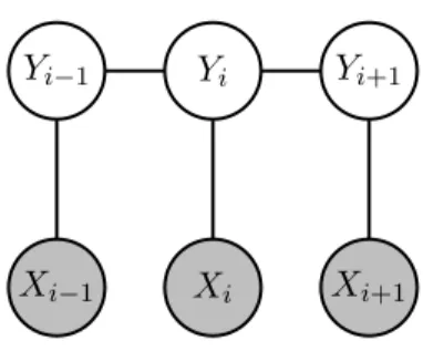
Figure 2.2: A first-order chain-linear CRF. The gray circles are the input words and are not generated by the model.

CRFs are undirected graphical models, introduced by Lafferty et al. for sequence predic-tion [40]. When the graph is a tree (as is usually the case in sequence predicpredic-tion) the joint probability distribution over the label sequence y given input x takes the form of Equation 2.1 p(y|x, λ) = 1 Z(x)exp m ∑ i=1 n ∑ j=1 λjfj(yi−1, yi, x, i) (2.1)

where the outer sum is over each example i in the sentence x and the inner one over each feature function fj. A feature function takes as input the previous label, the current label,

the examples x and the position i of the current example5_{. The output of the feature function} can be a real number but is usually binary.

It is the data scientist’s job to provide these feature functions as they are highly dependent on context. An example of these can be seen in Equation 2.2 to model token sequences like “abdominal pain”, “chest pain”, …

fj(yi−1, yi, x, i) =

{

1, if yi−1 = ANATOMICAL and xi= “pain”

0, otherwise (2.2)

Z(x) is defined in Equation 2.3 and is used to normalize the exponentiation.

Z(x) = ∑ y∈Y m ∑ i=1 n ∑ j=1 λjfj(yi−1, yi, x, i) (2.3)

An estimation for the parameters λ is obtained by maximizing the conditional log-likeli-hood objective function (Equation 2.4) using an iterative algorithm such as gradient ascent.

λM L= arg max λ m ∑ i=1 log p(y|x, λ) (2.4)

Abacha and Zweigenbaum use a CRF with lexical and morphosyntactic features combined with semantic feature obtained using MetaMap [41].

In a recent project, ChemSpot, a CRF is combined with a dictionary-based method to form a sort of ensemble learning method to annotate natural language text. The input text is ran through the CRF and the dictionary independently [34]. The output of the system is 5_{By restricting the feature function’s input to a single previous label, a first-order linear-chain CRF is}

implemented but this need not be the case.

(31)

the merging of all annotations produced by both methods, the CRF being preferred in cases where there is an overlap. Building a similar system can be greatly simplified by using the Neji framework [42].

2.2.4 Support Vector Machines

Another supervised learning used by several NER systems [43, 44] is the Support Vector

Machine (SVM).

An SVM solves binary classification problems by tracing an hyperplane which maximizes the distance between examples which belong to different classes (positive and negative labels). This hyperplane is nothing more than a linear function wT_{x + b which implies that the data}

must be linearly separable to obtain reasonable performance.

The key innovation in SVMs was introduced by Boser et al. when it was suggested to apply the kernel trick so as to make it possible to learn a nonlinear decision boundary by tracing the hyperplane in a transformed feature space [45].

The kernel trick is the observation that the linear function used by SVM’s can be re-written as wTx + b = b + m ∑ i=1 αixTx(i) (2.5)

where α is the vector of coefficients. Writing the hyperplane this way enables the replacement of the dot product with a kernel function k(x, x(i)_{) = ϕ(x)}T_ϕ(x(i)₎ _{where ϕ(x) is a feature} function. This gives us the general form of SVM classifiers in Equation 2.6. A commonly used kernel is the Gaussian kernel.

f (x) = b +

m

∑

i=1

αik(x, x(i)) (2.6)

Such form enables computing the classifier using convex optimization techniques which are guaranteed to converge efficiently [36].

There is still the issue of SVMs being binary classifiers and sequence labeling being a multi-class problem. This can be solved by combining several binary SVMs in a one-vs-all or pairwise fashions [43]. In one-vs-all, the i-th SVM is trained with examples of the i-th class being the positive label and all other classes the negative. In pairwise, all classes are combined in pairs. The first class of the pair becomes the positive label and the second class the negative. All SVMs vote on a label and the label with the most votes is chosen as the final output.

2.2.5 Recurrent Neural Networks

As previously mentioned, CRFs and SVMs require feature functions to be provided by the data scientist. Other kinds of machine learning methods also usually require significant feature engineering. This is time consuming and the scientist requires domain knowledge. Even so, the selected features might prove not to be the most effective.

A collection of machine learning methods called deep learning make use of a structure inspired by biological neural networks called an artificial neural network. The main component of these networks is the artificial neuron. The output of these neurons is defined as y =

(32)

Input Layer

Hidden Layer

Output Layer

Figure 2.3: A graph representation of a 3-layer feedforward densely connected neural network. The vertices are the neurons and the edges the connections established among them. Each connection has a vector of weights w and biases b which are not shared with other neurons.

U

W

y

x h

Figure 2.4: A recurrent neural network. The edge flowing from h to itself indicates weight sharing: weights from the previous input example are passed on to the next one.

σ(wTx + b) where σ is a non-linear activation function such as the rectified linear unit

σ(x) = max(0, x). Figure2.3 shows a simple neural network.

In supervised learning tasks, these neural networks do something akin to principal compo-nent analysis by assigning larger weights to the neurons whose output improves performance therefore disposing of the need to do heavy manual feature engineering.

Recurrent Neural Networks (RNNs) are a family of neural networks which specialize in

processing sequences of values x(1)_{, . . . , x}(τ )_{. These neural networks use parameter sharing} to apply the model to sequences of different lengths and generalize across them. Sharing the weights across all words in the sentence enables the network to learn the rules of the text only once and with fewer parameters [36]. Figure 2.4 shows an RNN. The connections from the input and from the hidden layers of the previous word are parameterized by U and W respectively which are optimized during the training phase.

By combining two RNNs, one which moves forward from the start of the sequence and another which moves backwards from the end, a bidirectional RNN is obtained. This structure enables the joint RNN to combined dependencies from previous and following inputs. Such is the strategy employed by Mavromatis for disease extraction [46].

Most modern RNN implementations use the Long Short-Term Memory (LSTM) cell [47] to compute a neuron’s output and in the biomedical domain this is no exception [48, 49, 50]. These cells are probably one of the most significant development in RNNs. See Olah [51] and Goodfellow et al. [36] for in-depth analysis.

RNNs can also be combined with other machine learning methods. A powerful combina-tion is the LSTM-CRF which is a bidireccombina-tional LSTM RNN with a CRF as the output layer [48, 49]. This hybrid system besides capturing dependencies through the hidden layers also

(33)

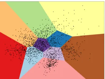
Figure 2.5: Generic clustering example. The dots could represent the tokens and the different colors the labels to which they were assigned e.g. “symptom”, “drug”, “disease”, etc.

captures label dependencies at the CRF layer. Unanue et al. show that pre-trained word embedding can improve the performance of this hybrid system [50].

A significant disadvantage of RNNs is that they experience very slow training. Because the output for an element in a sequence, besides depending on its input, is also a function of the previous element’s hidden layer, yt= f (xt, ht−1), RNNs can not be parallelized like other

neural networks.

2.2.6 Unsupervised Learning

An already stated disadvantage of supervised learning methods is that they require a pre-annotated (usually hand-annotated) corpus to use during the model’s training stage.

Unsupervised learning techniques experience features but not the supervision signal i.e. by

observing examples from the random vector x they learn the probability distribution p(x) [36]. These methods are not common in NER, much less in biomedical NER. A reason for this is that they are not as versatile as supervised learning techniques because they can not do term extraction. They can, although, still do term classification.

Clustering, as used by Elsner et al., is one such approach [52]. A representation of this

technique is illustrated in Figure 2.5.

The aim of clustering is to partition the examples x into k clusters according to some similarity metric using an algorithm like spherical k-means. Lin and Demner-Fushman use a variant of clustering called hierarchical agglomerative clustering where each entity starts with its own cluster that can then merge with another entity’s cluster when a common UMLS hypernym is shared among them [53]. Apirin and ibuprofen would be merged into the anti-inflammatory cluster which could be merged into the drug cluster.

Zhang and Elhadad use a customized approach where they collect “seed terms” from UMLS and assign them to classes such as “disease” [54]. A shallow syntactic parser is used to analyze the sentences. Each word is attributed a part-of-speech label and wanted labels — nouns — are kept. The similarity between these nouns and the seed terms is computed, through frequency of co-occurrence, to get their classification.

(34)

2.3 Relation Extraction

After using NER to extract relevant entities from text, the next step is to establish re-lations among those entities and other words in the sentence. For example, a connecting between a symptom and its cause as well as how confident the physician is in the association and the suggested treatment can be extracted.

A simple, rule-based, approach is to collect certain cue words and search for them in the vicinity of the named-entity using regular expressions. E.g., to determine the severity of a symptom, adjectives for intensity can be searched for [55]. This does not, however, make the system resilient to new vocabulary.

Following the trend in NER, more elaborate techniques use machine learning methods so much of the detailed in the NER section can now be applied to relation extraction.

Pathak et al. combine a dictionary with a CRF which uses bag-of-words, stem value and other feature functions [56]. SVMs prove to be common in the most effective relation extraction systems [57].

Other techniques are discussed in the following subsections.

2.3.1 Pointwise Mutual Information

In linguistics, a collocation is a sequence of words which co-occur somewhat frequently. Computing these collocations is therefore a way to extraction relations between terms based on their linguistic properties such as adjectives being followed by nouns.

Pointwise Mutual Information (PMI) is a way of measuring the association between the

terms and is defined as

P M I(x, y) = log p(x, y)

p(x)p(y) = log p(x|y)

p(x) (2.7)

where the probabilities p(x) and p(x_{|y) can be approximated by counting the occurrences and} co-occurrences of the words in the text.

PMI measures how much the probability of a certain co-occurrence p(x, y) differs from what would be expected based on the probability of individual events p(x) and p(y), assuming independence. Good candidates for collocation have high PMI.

Brujin et al. use data from the Medical Literature and Retrieval System Online (MED-LINE) to calculate how related two concepts are by finding collocations using PMI [58].

2.3.2 Deep Parsers

Shallow parsing was briefly mentioned in Section 2.2.2 as way of collecting tokens classified with the same part-of-speech into groups.

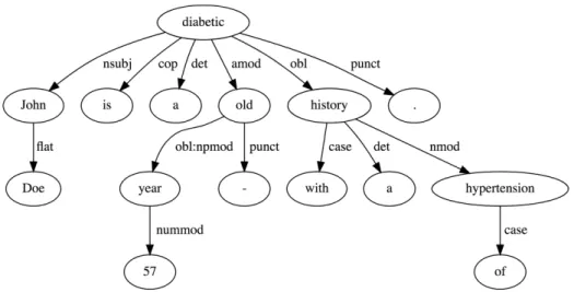
A more powerful form of syntactic parsing, deep parsing, besides assigning parts-of-speech to each word, also builds a dependency tree with the relations among the words in the sentence (Figure 2.6). This reveals the sentence’s semantic structure and, input into a machine learning model, functions as a powerful semantic feature. The tool to build these dependency trees is called a dependency parser. PALAVRAS is a significant example of a syntactic analyzer for the Portuguese language [59]. The current state-of-the-art dependency parser is Google’s SyntaxNet6_.

6_{https://github.com/tensorflow/models/tree/master/research/syntaxnet}

(35)

Figure 2.6: Dependency tree obtained using Google’s SyntaxNet for “John Doe is a 57 year-old diabetic with a history of hypertension”.

The winning entry for the Task 2 of SemVer’s 2014 Task 14 [60], UTH-CCB [61], uses a dependency tree, obtained using the Stanford Parser7, as one of the features input to an SVM classifier.

2.3.3 Convolutional Neural Networks

Sahu et al. [62] in a novel approach use another type of artificial neural network called a Convolutional Neural Network (CNN). CNNs specialize in modeling grid-like data such as images but they can be used with any kind of data such as text. What sets them apart from other neural networks is the usage of the convolution operation in at least one of their layers. Sahu et al. define the convolution as

s(t) = w· xi:i+c−1+ b (2.8)

where the notation xi:i+j _{represents the concatenation of feature vectors. This is similar to}

computing a linear activation in a regular neural network but with shared weights and biases, much like RNNs.

The difference is that the output of the convolution operation is a function of a small number of neighboring members of the input while in RNNs the output is a function of the previous members of the output. This makes RNNs better at generalizing for textual data but CNNs offset this disadvantage by experiencing much faster training due to their reduced number of parameters.

2.4 Classification

Yet another task in clinical text mining is statistical classification. This can be generally defined as the problem of assigning one or more labels to an observation. A classical example of this type of task is classifying e-mails as “spam” or “not spam”.

7_{https://nlp.stanford.edu/software/lex-parser.shtml}

(36)

A plethora of useful information can be obtained by classifying clinical text. Rajkomar et al. use three different models — a neural network, a LSTM and a time-aware neural network — to predict inpatient mortality, unplanned readmission, length-of-stay and diagnoses using EHR data from 216,221 patients from two different hospitals [7]. Garla et al. train an an SVM and a Laplacian SVM on a corpus of CT, MRI and Ultrasound reports labeled for the presence of malignant liver lesions that require follow up [63].

Medical coding is another task where text classification can be useful. Health facilities send patient data to insurance companies, for billing purposes, encoded in pre-established taxonomies like ICD, CPT and HCPCS. Assigning these codes to patient reports is done manually by medical personnel and automating this menial task is an ambition of researchers [64, 65].

Much like relation extraction, classification is mostly done with the already introduced machine learning techniques. Two of the mentioned publications do, although, introduce new concepts.

2.4.1 Semi-Supervised Learning

Semi-supervised learning is a mixture of supervised and unsupervised learning where an

algorithm, besides using examples x1, . . . , xl ∈ X with associated labels y1, . . . , yl ∈ X, is

also input unlabeled examples x_l+1, . . . , xl+u ∈ X. To usefully use the unlabeled data, it

is required to make an assumption about the structure of the underlying data distribution. Chapelle et al. lists four assumptions: the smoothness assumption, the cluster assumption, the manifold assumption and transduction [66].

The Laplacian SVM, used by Garla et al., adopts the manifold assumption and adapts the SVM to semi-supervised learning by defining a kernel function which uses unlabeled data [67]:

k′(x, x(i)) = k(x, x(i))− kx(I + M K)−1M kx(i) (2.9) where M is based on the Laplacian matrix L:

M = γI γAL

p _(2.10)

and k_x is a vector of kernel evaluations of x against all labeled and unlabeled training data. The parameters γI and γA specify a trade-off between regularization and deformation, weakening or strengthening the manifold assumption by shaping the feature space to reflect the manifold’s geometry.

2.4.2 Attention

The already presented LSTM cells used in RNNs aim to solve the problem of capturing long-term dependencies in sequences of various lengths. The recently developed mechanism of “attention” solves the same problem, although with much simpler modeling, by establishing a more direct dependence between states of the model at different points in time.

Rajkomar et al. learn attribution logits α, convert them to into weights Bi using the

softmax function and then use them to recalculate the weighed embeddings E =∑_jBjEj.

The calculation of attribution logits is done by Rajkomal et al. in a very problem specific way but Raffel and Ellis show a more general form:

αi = a(ht) (2.11)

(37)

where a is a learnable function which can be thought of as computing the scalar importance of ht[68].

As the authors suggest, this mechanism permits the modeling of long term dependencies, much like LSTM cells in RNNs, but with an added advantage. Assuming that ht= f (xt), no

dependency exists between hidden states which means that the model does not need to be trained sequentially, like an RNN, but can be trained in parallel like any other feed-forward neural network. A disadvantage which it does have, although, is that it requires yet another training process, this time for α. Additionally, Raffel and Ellis conclude that temporal order is discarded by the model, making the method inappropriate for some tasks.

(38)

(39)

Chapter 3

Classification of Clinical Reports

This chapter analyses the dataset, applied methods and their results.

3.1 Dataset

3.1.1 MIMIC-III

The Medical Information Mart for Intensive Care III (MIMIC-III) is a large, freely avail-able database of anonymized health-related data associated with patients of the intensive care unit (ICU) of the Beth Israel Deaconess Medical Center between 2001 and 2012 [69].

MIMIC-III is composed of several tables which host several types of data from admissions and transfers to patient information and test results. For the purposes of this thesis only two are used: the notes table (NOTEEVENTS) which contains reports input by clinicians and nurses into the EHR at each patient admission and the diagnosis table (DIAGNOSIS_ICD) which contains ICD-9-CM codes, associated with each admission, generated for billing purposes at the end of each patient’s hospital stay. Furthermore, diagnosis entries, and their associated notes, are only kept for patients who have been diagnosed with diabetes. This filtering adds up to a total of 406 190 reports which will be further reduced as indicated ahead in Section 3.1.3.

Before being made available to researchers, protected health information is removed through a thoroughly evaluated deidentification system based on dictionary look-ups and patterns matching with regular expressions [70]. Text which was changed during the deiden-tification process is surrounded with the pattern “[** **]”.

Each report in the notes table is assigned to one of fifteen categories:

• ECG • Nutrition • Radiology • Nursing • Discharge Summary • Rehab Services • Consult • Echo • Physician • General • Respiratory • Social Work • Nursing/Other • Pharmacy • Case Management

These categories are heterogeneous in their structure and language, much like already described in Section 2.1.1, which makes developing a technique for text classification that

(40)

[**2157-8-16**] 9:51 AM

UNILAT LOWER EXT VEINS LEFT Clip # [**Clip Number (Radiology) 106670**] Reason: Evaluate for DVT

Admitting Diagnosis: BILATERAL ADNEXAL MASS

__________________________________________________________________________ [**Hospital 2**] MEDICAL CONDITION:

75 year old woman with ovarian cancer, post op with left calf tenderness REASON FOR THIS EXAMINATION:

Evaluate for DVT

__________________________________________________________________________ FINAL REPORT

@@@@@@@@@@@@@@ is a revision of a previously signed report @@@@@@@@@@@@@@@ INDICATION: 75-year-old woman with ovarian cancer, postop with left calf tenderness. Evaluate for DVT.

COMPARISON: None.

FINDINGS: The common femoral, femoral and popliteal veins on the left demonstrate normal compressibility, augmentation, flow and respiratory variability. The vessels at the trifurcation are also compressible and appear patent. The posterior tibial amd peroneal veins are visualized and are compressible.

IMPRESSION: No evidence of DVT within the left leg.

Figure 3.1: Radiology report example. The pattern “[** **]” indicates the original text was replaced with an anonymized equivalent which keeps the text coherent. Note the lack of rich text formatting, usage of medical slang — “UNILAT”, “postop” — and a misspelling — “amd”.

generalizes to all of them particularly challenging. Figures 3.1 and 3.2, slightly formatted but otherwise copied verbatim, illustrate the differences between two categories of report.

3.1.2 ICD-9-CM

The disease labels associated with each report use the ICD-9-CM taxonomy. The Inter-national Statistical Classification of Diseases and Related Health Problems (ICD) is a disease classification system maintained by the World Health Organization. Although, at the time of this thesis’ publication, the most recent version is ICD-10, MIMIC-III uses the ninth revision of the codes with the Clinical Modification (CM). These codes are composed of three primary

Sinus rhythm. A-V conduction delay. Left atrial abnormality. Atrial and ventricular ectopy. Low limb lead voltage. Right bundle-branch block. Compared to the previous tracing of [**2183-4-17**] atrial and ventricular ectopy are recorded. The rate has increased. Otherwise, no diagnostic interim change.

TRACING #3

Figure 3.2: ECG (Electrocardiography) report example. Reports which belong to this cate-gory are usually short.

(41)

digits and either one or two optional digits which convey extra information. The Clinical

Modification augments ICD-9 with additional morbidity detail and with codes for surgical,

diagnostic and therapeutic procedures.

For the classification task, two different representations of the codes are considered. A regular one with codes which range from three to five digits and a rolled up version where all codes are limited to their first three (primary) digits.

The used MIMIC-III subset has 4006 different regular codes and 779 different rolled up codes. Each of the codes is used in labeling at least one report. Procedure codes are not used. The dataset has a very low label cardinality — defined as the average number of codes per report — of 17 for regular and 15 for rolled up labels. Label densities — define as the number of codes per report divided by the number of unique codes, averaged over the full dataset — are 0.0042 and 0.0198.

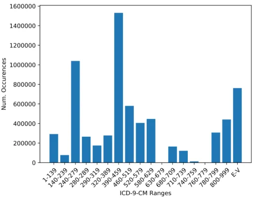
Figure 3.3 shows the number of occurrences for grouped ICD-9-CM codes. The group with the second most occurrences is “Endocrine, Nutritional and Metabolic Diseases, and Immunity Disorders”, which includes diabetes. This is preceded by “Diseases of the Circulatory System”, such as vascular and heart diseases. The overrepresentation of these very serious diseases, surpassing even diabetes, is attributed to the fact that the data was obtained from an ICU.

For each report, each code also has an associated sequence number which loosely ranks the relevancy of the codes to the patient’s stay.

Given the very high dimension of both the inputs — reports — and outputs — ICD-9 labels, whether rolled or not — this classification task can be considered to be a part of the eXtreme Multi-label Learning discipline.

3.1.3 Preprocessing

Preprocessing starts with a simple four step process which transforms each report into a sequence of tokens:

1. Punctuation characters, except for the apostrophe, are converted to whitespace

2. Digits are replaced by the character ’d’

3. All characters are converted to lowercase

4. The report is split at whitespace characters

As already noticed in Section 2.1.1, clinical text is prodigal of misspellings that can in-terfere with a classifier’s correctness. Baumel et al. suggest a simple vocabulary reduction step as a partial remedy [65]. Tokens that occur less than five times in the whole corpus are eliminated. These eliminated tokens are then mapped to their most similar token of the ones which were kept. The most similar token is defined as the one which minimizes the Levenshtein distance string metric:

leva,b(i, j) =

           max(i, j) if min(i, j) = 0 min      lev_a,b(i− 1, j) + 1 leva,b(i, j− 1) + 1

lev_a,b(i− 1, j − 1) + α

otherwise (3.1)

(42)

Figure 3.3: Number of occurrences for standardly grouped ICD-9-CM codes on the MIMIC-III subset. A reference for the grouping can be obtained from http://healthpolicy.ucla.edu/Documents/Spotlight/IDC9%20Groupings.pdf (visited on 30/03/2018).

(43)

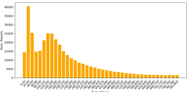
Figure 3.4: Report lengths in tokens for reports with sizes which range from 0 to 800. Most reports have from 20 to 40 tokens. Reports longer than 800 tokens are progressively fewer (not shown).

where a and b are the tokens, of length |a| and |b|, and α is a binary variable which is 1 if

ai = bj and 0 otherwise. The function is applied as leva,b(|a|, |b|). The python-Levenshtein

package was used1_.

The assumption for this step is that tokens which occur infrequently are misspellings of other tokens which occur more frequently. This does not always hold true but good results were observed, with the added advantage that the vocabulary was reduced from 162 784 to 53 229 unique tokens.

Most text classification tasks opt to use word embeddings to represent tokens. Word2vec’s skip-gram neural network model was input the corpus and used to generate three-hundredth dimensions word embeddings. The concrete implementation of word2vec used was the one from the gensim library2_{. Pre-trained word embeddings were also experimented with but} produced worse results due, most likely, to not containing enough domain specific terminology. Further preprocessing was necessary before inputting the data into the models. The Keras library, used to develop the models, expects fixed size inputs. As indicated, the lengths of the reports vary greatly, from 1 to 8513 tokens and, due to memory limitations, it would be infeasible to resize all sequences to the maximum length.

Figure 3.4 shows the number of reports for some length ranges. The majority of the reports has a relatively short length. It was chosen to keep only reports which have more than 9 and less than 2200 tokens. By doing this, 98.38% of the reports are kept unaltered and can fit in working memory while 6 567 are eliminated. The average length for the reports after this step is 309 tokens.

Table 3.1 summarizes the preprocessed dataset.

1_{https://github.com/ztane/python-Levenshtein/}

2_{https://radimrehurek.com/gensim/models/word2vec.html}

(44)

Num. of used records 399 623 Num. of regular labels 4 006 Num. of rolled up labels 779 Regular label cardinality 16.99 Rolled up label cardinality 15.39 Regular label density 0.0042 Rolled up label density 0.0198 Num. of unique tokens 53 229 Avg. num. of tokens per report 309.06

Table 3.1: Preprocessed dataset description.

Figure 3.5: Distribution of reports per category. The low number of reports for categories like Case Management and Consult is attributed to the fact that such event are rare in an ICU context.

3.1.4 Additional Analysis

Several statistics of the dataset were already calculated mostly to enable an informed preprocessing of the dataset. Here, further analysis is presented.

The distribution of these reports, per category, can be seen in Figure 3.5. Once again, great variability is observed. Nursing and Nursing/Other reports make up 44.19% of the total reports. This proliferation of nursing reports is in accordance to the guidelines of the American Association of Critical-Care Nurses which mandates periodic patient assessment from every few minutes for extremely unstable patient to at least every 2 to 4 hours for very stable patients [71]. Nursing reports are followed by all kinds of medical exams (Echo, ECG, Respiratory and Radiology) which make up 39.94% of the total reports. Noticeably, the Radiology category makes up almost one quarter of the total reports. As the single most commonly requested radiographic examination in ICUs is the portable chest radiograph, this is not surprising [72].

(45)

ICD-9-CM

Description %Reports

Code

250 Diabetes mellitus 100.00%

427 Cardiac dysrhythmias 46.64%

518 Other diseases of lung 45.53%

428 Heart failure 45.19%

584 Acute kidney failure 44.27%

401 Essential hypertension 43.47%

276 Disorders of fluid electrolyte and acid-base balance 38.74% 414 Other forms of chronic ischemic heart disease 37.40%

285 Other and unspecified anemias 35.10%

272 Disorders of lipoid metabolism 34.52%

585 Chronic kidney disease 27.05%

Table 3.2: The eleven most common rolled up ICD-9-CM codes.

Category Discharge Summary 250 401 414 272 427 428 276 285 584 V45 V58 Echo 250 414 428 427 401 272 584 276 285 518 585 ECG 250 428 427 414 401 272 584 276 285 518 403 Case Management 250 518 584 276 427 285 428 585 038 995 272 Respiratory 250 518 584 427 276 285 428 401 995 272 038 Nursing 250 584 518 427 276 428 285 272 401 414 585 Physician 250 518 584 276 427 428 285 272 401 585 414 Nutrition 250 518 584 276 427 285 428 401 272 995 585 Pharmacy 250 584 518 276 995 427 038 285 272 401 599 General 250 518 584 427 276 428 585 285 272 401 414 Social Work 250 584 276 518 427 285 428 585 401 414 272 Rehab Services 250 427 518 584 401 272 414 276 428 285 E87

Consult 250 427 518 428 285 276 585 401 584 403 E93

Radiology 250 401 427 584 518 428 276 414 272 285 V58

Nursing/Other 250 518 428 427 401 584 414 038 285 276 995

Table 3.3: The eleven most common rolled up ICD-9-CM codes per category. The codes are sorted left to right where the leftmost label — 250 — is the most common.

(46)

Tables 3.2 and 3.3 show the eleven most common labels globally (for the whole dataset) and per category. Unsurprisingly, the code 250 — diabetes mellitus — is always the most common. Whether comparing the global labels with the categories or the categories among themselves, it can be verified that, even though their arrangement changes, most of the ICD-9-CM codes are shared. If outliers were to be named they would be Case Management, Pharmacy and Consult with a mere two codes which do not show up in the global ones. This breaks the heterogeneity pattern, observed up to this point, by showing that, at least regarding the most common codes, the categories present some similarities.

Another pattern that shows up, related to this homogeneity, is that the Nursing, Physician, General and Social Work categories, not only share the exact same labels, but also a very similar disposition.

Table 3.2 also shows the percentage of reports which are classified with a each of the eleven most common codes. It can be seen that most of these codes have a somewhat balanced distribution with the most imbalanced being 585 at 27.05% positive targets.

3.2 Methods

3.2.1 Setup

To better understand how this problem can be solved and determine the most advanta-geous form of classification, two different methods are experimented with:

• Multi-label classification of the reports. Here, the classifier must learn to predict all ICD-9-CM labels assigned to each report. Separate classifiers are trained to predict labels in their regular and rolled up forms. For both forms, two variations of these models are considered. One where the model uses just the tokenized reports and another where, besides using the reports, it also takes as input the category of the report.

• Binary classification of reports for each of the most common rolled up labels (see Table 3.2). Here, each classifier is trained to predict a single label, contrasting with the previous task where a classifier predicts multiple labels. Both baseline and category augmented classifiers are also used.

Developing these classifiers mandates adopting a validation strategy to assess how well they generalize to an independent dataset. A popular approach with neural network based models is to split the dataset into training, test and validation subsets. The training set contains the examples the classifier uses to optimize its parameters; the validation set is used to measure the training effectiveness and to support regularization techniques, like early stopping; and the test set is used to provide an unbiased evaluation of the trained model. A disadvantage of this technique is that, by picking a fixed test set, the evaluation could be biased i.e. if a another test set was then picked it might produce significantly different results. An alternative is to use k-fold cross-validation. In this technique, the dataset is split into k more or less equal-sized subsamples. A single subsample is used for testing while the remaining k_{− 1 are used for training and validating. This process is then repeated k times} with each of the subsamples being used exactly once for testing. This means that k different results are obtained which can then be averaged to produce a final estimation, making this method a more resilient approach than the previously presented. Its disadvantage, that is non trivial when used with neural networks which typically experience long training times, is

(47)

Dense

Codes AveragePool

Embedding Reports

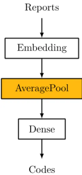
Figure 3.6: Baseline Bag-of-Tricks.

that the whole training process must also happen k times. A k of 5 was chosen and 10% of the k− 1 subsamples are used for validation.

The library and classifier architectures used impose some constraints on how the data is to be represented. Reports are encoded as a sequence of indexes which map to tokens in the known vocabulary; categories are encoded as a 1-hot vector where the category assigned to the report is positive; labels are encoded as a k-hot vector, where all labels assigned to the report are positive.

As already mentioned, the Keras library was used to develop the classifiers [73]. Keras provides a high-level interface to the lower-level neural network library Tensorflow [74], greatly easing development.

3.2.2 Bag of Tricks

The first method is a simple linear model based on Armand et al.’s Bag of Tricks (BoT) [75]. BoT uses a very similar architecture to Mikolov et al.’s Continuous Bag-of-Words [76] but is not limited to words and can classify arbitrary type labels.

The baseline version of this classifier can be seen in Figure 3.6. The embedding layer transforms the report’s tokens into high dimension word embeddings. These embeddings are then averaged into a fixed dimension vector before being fed into a dense/fully-connected layer. The size of the dense layer varies according to the task: 4 006 for regular multi-label classification, 779 for rolled up label classification and 1 for binary classification.

The significant departure from Armand et al. is in the usage of the sigmoid activation function (Equation 3.2) at the dense layer’s outputs instead of the softmax function. Softmax squashes the layer’s inputs into a probability distribution which would not be appropriate in a multi-label scenario as labels are not mutually exclusive e.g. both “diabetes” and “heart arrhythmia” can be assigned to a single report. The sigmoid function, instead, squashes each neuron’s input into a value in the range [0_{− 1] so that each neuron outputs a Bernoulli} probability distribution independent of all other neurons. To determine if the neuron’s label