A NEW METHOD FOR DECISION MAKING IN MULTI-OBJECTIVE OPTIMIZATION PROBLEMS
Oscar Brito Augusto
1*, Fouad Bennis
2and Stephane Caro
3Received June 21, 2010 / Accepted March 12, 2012
ABSTRACT.Many engineering sectors are challenged by multi-objective optimization problems. Even if the idea behind these problems is simple and well established, the implementation of any procedure to solve them is not a trivial task. The use of evolutionary algorithms to find candidate solutions is widespread. Usually they supply a discrete picture of the non-dominated solutions, a Pareto set. Although it is very interesting to know the non-dominated solutions, an additional criterion is needed to select one solution to be deployed. To better support the design process, this paper presents a new method of solving non-linear multi-objective optimization problems by adding a control function that will guide the optimization process over the Pareto set that does not need to be found explicitly. The proposed methodology differs from the classical methods that combine the objective functions in a single scale, and is based on a unique run of non-linear single-objective optimizers.
Keywords: multi-objective optimization, multi-attribute decision making, engineering design optimiza-tion.
1 INTRODUCTION
Many engineering design problems are multi-objective in nature as they often involve more than one design goal to be optimized. These design goals potentially impose conflicting requirements on the technical and economic performance of a given system design. To study the trade-offs between these conflicting design objectives and to explore design options, an optimization prob-lem with multiple objectives has to be formulated. To facilitate the exploration of different multi-objective formulations, we can incorporate Pareto optimality concepts into optimization algorithms that require the designer’s involvement as a decision maker.
Edgeworth (1881) was the first academic to define an optimization problem involving multiple criteria. The problem, elaborated in the context of two consumers called P andπcan be defined
*Corresponding author
1Escola Polit´ecnica da Universidade de S˜ao Paulo. E-mail: [email protected]
2 ´Ecole Centrale de Nantes, Institut de Recherche en Communications et Cybern´etique de Nantes. E-mail: [email protected]
as: “it is required to find a point(x,y)such that, in whatever direction we take an infinitely step, P andπdo not increase together, but, while one increases, the other decreases”.
A few years later, in 1896, Pareto (1971) establishes the optimum for n consumers: “we will say that members of a collectivity enjoy maximum ophelimity in a certain position when it is impossible to find a way of moving from that position very slightly in such a manner that the ophelimity enjoyed by each of the individuals of that collectivity increases or decreases. That is to say, any small displacement in departing from that position necessarily has the effect of increasing the ophelimity which certain individuals enjoy, and decreasing that which other enjoy, being agreeable to some and disagreeable to others”.
Since then, many researchers have been dedicated to developing methods to solve this kind of problem. Interestingly, solutions for problems with multiple objectives, also called multi-criteria optimization or vector optimization, are treated as Pareto optimal solutions or Pareto front, al-though as Stadler observed (1988), they should be treated as Edgeworth-Pareto solutions.
On the other hand, thanks to the evolution of computers, the optimization of large scale problems has become a common task in engineering design processes. Computers, ever faster, with higher capacity of data storage and Internet connection capability, are revolutionizing the traditional ways of developing engineering designs. Currently, engineers can rely on a wide range of design alternatives and optimization methods that allow systematic choices between alternatives when they are based on measurable criteria. Used properly, these methods can improve or even gen-erate the final solution of a design, as shown in Giassiet al. (2004), which held multi-objective optimization of a vessel hull shape with collaborative design method where the computational tools for the analysis of alternatives used in the cycles of optimization were distributed in three different sites. With this approach they demonstrate that if the optimization is conducted in a distributed way it becomes a powerful tool for the concurrent design.
Raoet al. (2007) designed a disk for high-pressure turbine aircraft engines, treating the prob-lem as multi-objective by considering the manufacturing cost and fatigue life as functions to be optimized. Bouyer et al. (2007) performed the optimal design of a mechanical transmission system,Slide-O-Cam, which turns rotary into translation motion and replaces the conventional rack-pinion systems, a problem with four objective functions. In both instances, the optimal solutions were presented by their Pareto fronts.
Plenty of methods for solving design problems with more than one objective are found in scien-tific and technical literature. However, since the multi-objective problems have no single solution but a set of points called optimal solutions, the question that arises ishow to choose one alter-native among those contained in the set of solutions. The answer is not simple unless another criterion is added to help choose the alternative that should be deployed.
the control function over the Pareto set that would result from the optimization problem con-stituted by the group of performance functions if this multi-objective optimization problem had been solved. However, since this task is not performed, the Pareto front is not an output of the optimization process and the computational task is significantly smaller than the traditional multi-objective optimization algorithms.
Applying this strategy to a multi-objective optimization problem requires the use of an algorithm that can solve a single-objective problem and work with the functions involved. The result will be a single solution. However, the methodology differs significantly from other classical algo-rithms as there is no need to know a value function relating the objectives that articulates de designer preferences.
After this brief introduction, the remaining of the paper is organized into six sections. The first formulates a general multi-objective optimization problem and defines the nature of optimal so-lutions from the Pareto perspective and the necessary conditions to be met. The second presents a brief literature review on multi-objective optimization problem algorithms. In the sequence, it presents the main contribution of this work, a new strategy to solve the optimization prob-lem with multiple objectives. Next, it goes on to the impprob-lementation of the strategy to solve three problems with increasing levels of complexity, and finally presents the conclusions on the work done.
Nomenclature
AIS artificial immune systems AC ant colony optimization algorithm
DM decision maker
fi(X) ithobjective function
fc(X) control function
fio(X) minimum value of the ithobjective function fimax(X) maximum value of the ithobjective function
tolf tolerance for equal values ofrmsin successive generations f(X) objective functions vector
fp(X) performance functions vector
fo ideal point, vector with all objective functions’ minima, in criterion space
GA genetic algorithm
gj(X) jthinequality constraint function
hi(X) ithequality constraint function
k number of objective functions
KKT Karush-Khun-Tucker
l number of equality constraint functions
m number of inequality constraint functions MOOP multi-objective optimization problem
n dimension of the design space
p number of performance functions
PS particle swarm optimization algorithm
r msn root mean square of all objective functions at the nthgeneration Rk function or criterion space
Rn decision variables or design space
SA simulating annealing optimization algorithm S feasible region in the design space
VEGA vector evaluated genetic algorithm
xi ithdecision variable
xi average of the ithdecision variable included in the optimal set
X decision variable vector
X∗ non-dominated solution of a multi-objective optimization problem Xinf,Xsup lower and upper bounds of the design space
Xextended extended vector for unknowns withX,α,λandµ
αi weighting factor for ithobjective function gradient in KKT condition
α vector ofαi s
ωi weighting factor for the ithobjective function
ω∗i normalizing weighting factor for the ithobjective function
εj upper bound for the jthobjective function in theε-restricted method
λj weighting factor for jthinequality constraint gradient in KKT condition
λ vector ofλj s
σi standard deviation for the ithdecision variable included in the optimal set
μi weighting factor for ithequality constraint gradient in KKT condition
µ vector ofμi s
∇ gradient operator
2 MULTI-OBJECTIVE OPTIMIZATION PROBLEM
Multi-objective optimization problems (MOOP) can be defined by the following equations:
minimize: f(X) (1a)
subject to: gi(X)≤0, i=1,2, . . .m. (1b)
hj(X)=0, j =1,2, . . . ,l. (1c)
Xinf≤X≤Xsup (1d)
where
f(X)=
f1, f2, f3, . . . , fk T
:X→Rk
Xsupare respectively the lower and upper bounds of the design variables.gi(X)represents the ith inequality constraint function andhj(X)the jthequality constraint function. The three equations (1b)-(1d), define the region of feasible solutions,S, in the design spaceRn. The constraintsgi(X)
are of type “less than or equal” functions in view of the fact that “greater or equal” functions may be converted to the first type if they are multiplied by−1. Similarly, the problem is the “minimization” of the functions fi(X), given that functions “maximization” can be transformed into the former by multiplying them by−1.
2.1 Pareto optimal
The notion of “optimum” in solving multi-objective optimization problems is known as “Pareto optimal.” A solution is said to be Pareto optimal if there is no way to improve one objective without worsening at least one other,i.e., the feasible pointX∗ ∈ Sis Pareto optimal if there is no other feasible pointX∈ Ssuch that∀i,j withi 6= j, fi(X)= fi(X∗)with strict
inequality in at least one condition, fj(X) < fj(X∗).
Due to the conflicting nature of the objective functions, the Pareto optimal solutions are usually scattered in the regionS, a consequence of not being able to minimize all the objective func-tions simultaneously. In solving the optimization problem we obtain the Pareto set or the Pareto optimal solutions defined in the design space, and the Pareto front, an image of the objective functions, in the criterion space, calculated over the set of optimal solutions.
2.2 Necessary condition for Pareto optimality
In fact, optimizing multi-objective problems expressed by equations Eqs. (1a)-(1d) is of general character. The equations represent the problem of single-objective optimization whenk = 1. According to Miettinen (1998), such as in single-objective optimization problems, the solution X∗ ∈ Sfor the Pareto optimality must satisfy the Karush-Kuhn-Tucker (KKT) condition, ex-pressed as:
k X
i=1
αi∇fi(X∗)+ m X
j=1
λj∇gj(X∗)+ l X
i=1
μi∇hi(X∗)=0 (2a)
λjgj(X∗)=0 (2b)
λj ≥0 (2c)
μi ≥0 (2d)
αi ≥0; k X
i=1
αi =1 (2e)
i.e.,gj(X∗) >0.μi represents the weighting factor for the gradient of the ithequality constraint function,∇hi(X∗).
The set of Eqs. (2a) to (2e) form the necessary conditions for X∗ to be a Pareto optimal. As described by Miettinen (1998), it is sufficient for the complete mapping of the Pareto front if the problem is convex and the objective functions are continuously differentiable in theSspace. Otherwise, the solution will depend on additional conditions, as shown by Marler and Aurora (2004).
3 LITERATURE REVIEW IN METHODS FOR SOLVING MOOP
Some researchers have attempted to classify methods for solving MOOP according various con-siderations. Hwang & Masud (1979) and later Miettinen (1998) suggested the following four classes, depending on how the decision maker (DM) articulates preferences: no-preference meth-ods,a priorimethods,a posteriorimethods, and interactive methods.
In no-preference articulation methods, the preferences of the DM are not taken into consideration. The problem can be solved by a simple method and the solution obtained is presented to the DM which will accept or reject it.
Ina prioripreference articulation methods, the hopes and opinions of the DM are taken into con-sideration before the solution process. Those methods require that the DM knows beforehand the priority of each objective transforming the multi-objective problem in a single-objective problem where the function to be optimized is a combination of objective functions.
In posteriori preference articulation methods no preferences of the DM are considered. After the Pareto set has been generated, the DM chooses a solution from this set of alternatives.
In interactive preference articulation methods the DM preferences are continuously used during the search process and are adjusted as the search continues.
Before explore the basics of some MOOP algorithms, it is opportune to define the ideal point
fo=f1o, f2o,f3o, . . . , fkoT
∈Rk
being fiothe minimum of fi(X),X∈Sandi =1,2, . . . ,k. In general,fois unattainable,i.e., such a point in the criterion space does not map to a point in the design space.
In many cases it is advantageous to transform the original objective functions. This is especially true with scalarization methods that involvea prioriarticulation of preferences. As the objective functions usually have different scales, it is necessary to transform them in a non-dimensional. The relation
fis(X)= fi(X)
fio (3)
Alternatively, a most robust approach would be
fis(X)=
fi(X)− fio
fimax− fi0 (4)
with fimax, the maximum value of fi(X)forX∈ S. This operation is referred as normalization as the transformed function is bounded into the zero-one interval.
3.1 The weighted sum method
One of the most intuitive ways used to obtain a single unique solution for multi-objective opti-mization is the weighted sum method. In this approach, the MOOP are converted into a scalar preference function using a linear weighted sum function of the form,
minimize: k X
i=1
ωifis(X) (5a)
subject to: X∈S (5b)
ωi ≥0; k X
i=1
ωi =1 (5c)
For this method, the weightsωi reflect,a priori, the designer’s preferences. It is simple, but the proper selection of the weights may be a challenge itself.
The method can be used to find the Pareto set in many individual runs if the weights are consis-tently chosen for each run. Nevertheless, varying the weights continuously may not necessarily result in an even distribution of Pareto optimal points and a complete representation of the Pareto optimal set for non-convex problems as shown in Miettinen (1998).
3.2 The weighted metric methods
Other means of combining multiple objectives into a single-objective are based on the weighted distance metrics. Some DMs aim to find a feasible design that minimizes its distance from a pre-defined design as the representation of a designer’s overall preferences. Assuming that the pre-defined design is the ideal design, the weighted p-norm as is expressed by
lp= k X
i=1
ω∗i|fi− fio| p
!
1
p
(6)
where,
ωi∗= ωi fimax− fio
The MOOP is written as
minimize: lp (7a)
subject to: X∈S (7b)
ωi ≥0; k X
i=1
ωi =1 (7c)
The parameter pmay be chosen from 1 to infinite. With p =2, Eq. (6) yields to the Euclidian distance metric.
A compromise solution, an alternative to the idea of Pareto optimality is a single point that minimizes the Euclidian distance between the potential optimal point and the ideal point.
3.2.1 The min-max method
The min-max solution was initially proposed by Lightner and Director (1981). The method try to find a feasible design that minimizes its distance from the ideal design as the representation of a designer’s overall preferences. The weighted∞-norm is used as distance metric.
In Eq. (6), the limit oflpas papproaches to∞is
l∞=lp→∞
yields
−→max i
ωi∗|fi− fio|
(8)
because the largestωi∗(fi− fio)will dominate all others when taken to the infinite power.
The min-max problem is then defined by
minimize: max
i
ωi∗|fi − fio|
(9a)
subject to: X∈S (9b)
Given different relative weights of objectives, the min-max method is capable of discovering efficient solutions of a multi-objective problem whether the problem is convex or non-convex.
3.3 The goal programming
Goal programming, originally proposed by Charnes & Cooper (1977), is a technique which requires preference information before any efficient solution are generated. In fact, the method requires a designer to set goals,bi for all objectives, fi, that he wishes to achieve. It adopts the decision rule that the best compromise design should be the one which minimizes the weighted sum of deviations from the set goals, Pk
i=1ω∗i|di|, wheredi is the deviation from the goalbi for the ith objective. To model the absolute values, d
been reached. Similarly, the jth-inequality or equality constraint function are treated like the objective functions setting the goalsbj =0. Then, the MOOP is formulated as:
minimize: k X
i=1
ω∗i(di++di−) (10a)
subject to: fi(X)+di++di−=bi, i =1,2, . . . ,k (10b)
di+≥0, di−≥0 and di+di−=0, i=1,2, . . . ,k (10c)
ωi ≥0 (10d)
X∈S (10e)
The method allows the designer to assign preemptive weights to objectives and to define different achievement levels of the goals.
3.4 Theε-constraint method
Haimeset al. (1971) introduced theε-constraint strategy that minimizes the single objective function fi(X). All other objective functions are used to form additional constraints. The MOOP is formulated as:
minimize: fi(X) (11a)
subject to: fj(X)≤εj, j =1,2, . . . ,k; ∀j 6=i (11b)
X∈S (11c)
The definition of the limits εj requires knowinga priorithe designer’s preference. A set of Pareto optimal solutions can be obtained with a systematic variation ofεj. However, improper selection ofεj ∈Rcan result in a formulation with no feasible solution.
3.5 Nature inspired metaheuristic algorithms
The methods for multi-objective optimization presented thus far have involved unique formula-tions that are solved using standard optimization engines or single-objective optimization meth-ods algorithms. With those methmeth-ods, only one Pareto optimal solution can be expected to be found in one simulation run of a classical algorithm and not all Pareto optimal solution can be found by some algorithms in non-convex MOOP.
However, other approaches such some heuristics inspired in nature process can solve MOOP getting the Pareto set directly.
3.5.1 Genetic algorithms
extinction by natural selection. The strong ones have greater opportunity to pass their genes to future generations via reproduction. In the long run, species carrying the correct combination in their genes become dominant in their population. Sometimes, during the slow process of evolution, random changes may occur in genes. If these changes provide additional advantages in the challenge for survival, new species evolve from the old ones. Unsuccessful changes are eliminated by natural selection.
The concept of GA was originally proposed by Holland (1974) for applications into the control theories and it was quickly generalized to many different areas of engineering and sciences. The specific mechanics of the algorithm involve the language of microbiology and, in developing new potential solutions, mimic genetic operations. Apopulationrepresents a group of potential solu-tion points. Agenerationrepresents an algorithmic iteration. Achromosomeis comparable to a design point, and ageneis comparable to a component of the design vector. Given a population of designs, three basic operations are applied: selection,crossover, andmutation. The selection operator involves selecting design vectors, calledparents, in the current generation, which are combined together, by crossover, to form new chromosomes, called offspring. By iteratively applying the crossover operator, genes of good chromosomes are expected to appear more fre-quently in the population, eventually leading to convergence to an overall good solution. The mutation operator introduces random changes into characteristics of chromosomes. Mutation reintroduces genetic diversity back into the population and assists the search escape from local optima.
Being a population-based approach, GA is well suited to solve multi-objective optimization prob-lems finding a set of multiple non-dominated solutions in a single run. The ability of GA to simultaneously search different regions of a solution space makes it possible to find a diverse set of solutions for difficult problems with non-convex, discontinuous, and multi-modal solu-tions spaces. In addition, most of multi-objective algorithms do not require the user to prioritize, scale, or weigh objectives. Consequently, GA has been the most popular heuristic approach to multi-objective design and optimization problems. Coello (2010) maintains an updated list with more than 5000 titles of publications involving different genetic algorithms.
The first multi-objective genetic algorithm, calledvector evaluated genetic algorithm, or VEGA, was proposed by Schaffer (1985). Afterwards, several multi-objective evolutionary algorithms were developed, as shown by Konaket al. (2006), including the one that is used in this work to compare problems’ results, thenon-dominated sorted genetic algorithm, or NSGA II, proposed by Debet al.(2000).
distance. During selection, the NSGA II uses a crowded-comparison operator which takes into consideration both the non-domination rank of an individual in the population and its crowding distance. The non-dominated solutions are preferred over dominated solutions, but between two solutions with the same non-domination rank, the one that resides in the less crowded region is preferred. The NSGA II uses the elitist mechanism that consists of combining the best parents with the best offspring obtained. Goldberg (1989) and Deb (2001) are excellent guides for GA implementations.
3.5.2 Particle swarm
Particle swarm optimization algorithm (PS) was originally proposed by Kennedy & Eberhart (1995). It is a population-based search algorithm based on the simulation of the social behavior of birds within a flock. Although originally adopted for balancing weights in neural networks, PS soon became a very popular global optimizer.
There are two main distinctions between PS and GA. Genetic algorithms rely on three mecha-nisms in their processing. In contrast, PS only relies on two mechamecha-nisms, since PS does not adopt an explicit selection operator. The absence of a selection mechanism in PS is compensated by the use of leaders to guide the search. Such set of leaders is usually stored in a different place in an external archive, with all non- dominated solutions found so far. However, there is no notion of offspring generation in PS as with evolutionary algorithms. A second difference has to do with the way in which the individuals are manipulated. PS uses an operator that sets the velocity of a particle to a particular direction. This can be seen as a directional mutation operator in which the direction is defined by both the particle’s personal best and the global best of the swarm. If the direction of the personal best is similar to the direction of the global best, the angle of potential directions will be small, whereas a larger angle will provide a larger range of exploration. In con-trast, evolutionary algorithms use a mutation operator that can set an individual in any direction, although the relative probabilities for each direction may be different.
The main algorithm of PS is relatively simple, it only adopts one operator for creating new solutions and its implementation is, therefore, straightforward. Its main drawback is how to control de size of the external archive that implies in the computational time expended in the optimization process.
3.5.3 Simulated annealing
Serafini (1985, 1992). The algorithm of the method is almost the same as the algorithm of single objective SA. The slow convergence rate for some optimization problems is the main drawback of SA, as mentioned by Suman & Kumar (2006).
3.5.4 Ant Colony optimization algorithm
The ant colony optimization algorithm (AC) is inspired by the behavior of ants and other insects that live in a colony that in spite of the simplicity of each individual, present a high level of social organization when observed together. Some examples of ant colony’s capabilities found in Dorigoet al.(1999) are: division of labor and task allocation, cemetery organization and brood sorting, cooperative transport and finding the shortest path between two or more locations, often between a food source and a nest.
The first AC algorithm developed was initially applied to the traveling salesman problem, Dorigo (1992). The algorithm was based on the ant colony capability to find the shortest path between a food source and a nest. The algorithm uses artificial ants that cooperate on finding solutions to the problem through communication mediated by artificial pheromone trails.
While moving on the graph associated with the problem, artificial ants deposit pheromone on the edges traversed marking a path that may be followed by other members of the colony, which then reinforce the pheromone on that path. With this kind of communication, ants have their activities coordinated. This self-organizing behavior results in a self-reinforcing process that leads to the formation of a path marked by high pheromone concentration, while paths that are less used tend to have a diminishing pheromone level due to evaporation.
This concept can be applied to any combinatorial optimization problem for which a constructive heuristic can be defined. The process of constructing solutions can be regarded as a walk on a construction graph where each edge of the graph represent a possible step the ant can take. AC is essentially constructive, as ants generate solutions by adding solution components, correspond-ing to the edges chosen, to an initially empty solution until the solution is complete.
3.5.5 Artificial immune systems
The human immune system has as its main task the detection of the infectious foreign elements, called pathogens, that attack us, and defend us from them, i.e., its main task is to keep our organism healthy. Examples of such pathogens are bacteria and viruses. Any molecule that can be recognized by our immune system is called antigen. Such antigens provoke a specific response from our immune system. Lymphocytes of types B and T are special type of cells that play a major role in our immune system.
mutations experienced by the clones are proportional to their affinity to the antigen. The highest affinity cloned cells experiment the lowest mutation rates, whereas the lowest affinity cloned cells have high mutation rates. Due to the random nature of this mutation process, some clones could be dangerous to the body and are, therefore, eliminated by the immune system itself. Plasma cells are capable of secreting only one type of antibody, which is relatively specific for the antigen. Antibodies play a key role in the immune response, since they are capable of adhering to the antigens, in order to neutralize and eliminate them.
Once the antigens have been eliminated by the antibodies, the immune system must return to its normal conditions, eliminating the in-excess cells. However, some cells remain in our blood stream acting as memory cells, so that our immune system can ‘remember’ the antigens that have previously attacked it.
When the immune system is exposed again to the same type of antigen or a similar one, these memory cells are activated, presenting a faster and perhaps improved response, which is called secondary response.
Based on the previous explanation of the way in which human immune system works, it can be say that, from a computer science perspective, the immune system can be seen as a parallel and distributed adaptive system. Clearly, the immune system is able to learn, it has memory, and is able of tasks such as associative retrieval of information. These features make immune systems very robust, fault tolerant, dynamic and adaptive. All of these properties can be emulated in a computer.
Artificial immune systems (AIS) are composed of the following basic elements: a) a represen-tation for the components of the system,e.g., binary strings, vectors of real numbers; b) a set of mechanisms to evaluate the interaction of individuals with their environment and with each other; such an environment is normally simulated through an affinity function, which is based on the objective functions in the case of optimization problems; c) procedures of adaptation, that indicate the way in which the behavior of the system changes over time; these procedure of adaptation consist of, for example, mutation operators.
The first direct use of the AIS for multi-objective optimization goes back to Yoo & Hajela (1999). In their work they use a standard genetic algorithm where the immune principle of antibody-antigen affinity is employed to modify the fitness value. In a first time the population is evaluated
versusthe problem objectives and different scalar values are obtained by making reference to different weighting combinations. The best individual with respect to each combination is identi-fied as antigen. The rest of the population is the pool of antibodies. Then antibodies are matched against antigens by the definition of a matching score. The best matching antibody fitness is added by this matching score, evolving the population of antibodies to cover antigens.
4 DECISION MAKING IN MULTI-OBJECTIVE OPTIMIZATION PROBLEMS
criteria are necessary to select a single solution that will be deployed. Even though useful to better understand the inter-relationships between the objectives, the Pareto front may become an obstacle since just one solution must be implemented. To make a selection, the DM will have to use an additional criterion, be it subjective or not.
Then, why not formalize and include this additional criterion into the problem and make it a
control functionto find the single and final solution to be deployed among those that belong to Pareto front?
Based on this idea, we propose a new methodology to formulate MOOP involving non-linear differentiable functions. The method transforms the MOOP from multi-objective into single-objective that can be solved with the aid of any traditional single-single-objective optimization engine suitable for the problem in focus.
4.1 Proposal of a new methodology for decision making in MOOP In the proposed method, the objective functions are divided into two groups:
a) thecontrol function group, or simply,control function, which contains only one function.
b) theperformance functions group, which is made up of the functions that will provide the Pareto set.
Which function will be part of each group is a designer’s choice and depends on his or her expe-rience and knowledge related to the design problem. The control function can be an additional objective function or it can be elected among the problem objective functions.
The performance functions will have an important role in the process as they will provide the Pareto set as a constraint over which the control function will search the solution that optimizes it.
Thus, the multi-objective optimization problem can be written as:
minimize: fc(X),fp(X) (12a)
subject to: gi(X)≤0, i =1,2, . . . ,m (12b)
hj(X)=0, j =1,2, . . . ,l (12c)
Xinf≤X≤Xsup (12d)
where fc(X)is thecontrol function,
fp(X)=f1, f2, . . . , fp:X→Rp
is the vector composed of the pobjective functions in theperformance functions group.
It should be noted that the weighting factors of the Eq. (2a),i.e.,
α=
α1, α2, . . . , αp T
, λ=
λ1, λ2, . . . , λm T
and µ=
μ1, μ2, . . . , μl T
are not known. As unknowns in the problem, they will be incorporated into the vector of design variables, defining the extended vector of unknowns:
Xextended =(X,α, λ, µ) (13) Finally, the problem is formulated as a single-objective optimization problem, with the control function, fc(X), to be minimized and constrained by the conditions for obtaining the Pareto optimal solutions considering only the performance functions, f1(X),f2(X), . . . ,fp(X). Mathematically, the optimization problem is formulated as:
findXextendedthat
minimizes: fc(X) (14a)
subject to:
Pareto set condition for the performance functions:
p X
i=1
αi∇fi(X)+ m X
j=1
λj∇gj(X)+ l X
i=1
μi∇hi(X)=0
gi(X)≤0, i =1,2, . . . ,m
hj(X)=0, j =1,2, . . . ,l
λjgj(X)=0
λj ≥0
μi ≥0
αi ≥0; p X
i=1 αi =1
Xinf≤X≤Xsup
(14b) (14c) (14d) (14e) (14f) (14g) (14h) (14i)
The proposed methodology differs from those methods exposed in the items 3.1 to 3.4. Those strategies require that a complete decision-making structure of the problem is decideda priori. Although the proposed method is also based ona prioridecisions, just one function shall be added or isolated as a control function. The remaining functions are incorporated into the for-mulation to ensure that the final solution is within the Pareto set obtained from the minimization problem of these functions, even though the Pareto set and the Pareto front is not an explicit outcome of the process.
obtained is a local optimum and it can be a global optimum for convex Pareto fronts, since Eq. (2a) is a necessary condition for the existence of an extreme point and not a sufficient condition.
5 APPLICATIONS
To validate the proposed multi-objective optimization method, it will be used to solve three ex-amples with increasing levels of complexity, namely the optimization problem of three quadratic functions, the design of a cantilever beam and the conceptual design of a bulk carrier.
To solve the single-objective optimization problem originated by the proposed methodology, any algorithm that works with optimization problems involving nonlinear functions and constraints can be used. Due to its accessibility, the solverfmincon was used. It is a component of the
Optimization Toolboxavailable in the application MatLab, Matworks, version 7.1.
The NSGA II was used to compare results and to show that the results of the proposed method lay over the Pareto set from the MOOP of the performance functions group. A minor adaption was done in the NSGA II in order to interrupt the evolution if there is no significant difference between consecutive generations. Calling f ij the value of the ith objective function for the jth chromosome at nth generation of a population withpopchromosomes, the root mean square of the objective functions for the population can be defined as
r msn =
2
v u u t k X
i
Ppop j f ij
2
f imax− f imin2
(15)
with f imax and f imi nbeing the maximum and the minimum value, respectively, of the ith objec-tive function evaluated in the population. The alternaobjec-tive stop criterion was defined as
|r msn−r msn−1| ≤tolf ∙r msn−1 (16)
where tolf is a small number. Sometimes, for a defined tolf value, this criterion may cause a premature interruption of the evolutionary process. To overcome this situation, the algorithm checks if it occurs in subsequent generations before discontinue the evolution. As a default, three subsequent generations were adopted with the satisfaction of Eq. (16) as the condition to interrupt the evolutionary process.
5.1 Minimization of three quadratic functions Consider the minimization problem defined by:
minimize: f1(x1,x2)=3(x1+5)2+(x1+5)(x2−2)+(x2−2)2 (17a)
f2(x1,x2)=(x1−5)2−(x1−5)(x2−3)+(x2−3)2 (17b)
Assume that the functions f1(x1,x2)and f2(x1,x2)integrate the performance functions group
and the function f3(x1,x2)is the control function. Accordingly, the problem can be formulated
as:
findXextended =x1,x2, α1, α2T
that
minimize: fc(x1,x2)=(x1+2)2+(x2+6)2 (18a)
subject to: α1∇f1(x1,x2)+α2∇f2(x1,x2)=0 (18b)
αi ≥0;
2
X
i=1
αi =1 (18c)
The solution of this problem,(x1,x2, α1, α2)=(−1.1142,−0.0226,0.3019,0.6981), is shown
in Table 1 and in the Figure (1a). The point that minimizes the control function falls into the Pareto set resulting from the MOOP formed by the performance functions. The Pareto sets shown in Figures (1a)-(1e) are not obtained by the methodology and they were computed for comparison only by a suitable algorithm.
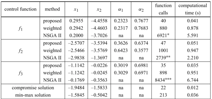
Table 1– Results for the minimization of quadratic functions.
control function method x1 x2 α1 α2
function computational calls time (s) proposed 0.2955 –4.4558 0.2323 0.7677 40 0.041
f1 weighted 0.2942 –4.4603 0.2317 0.7683 880 0.878 NSGA II 0.2000 –3.7026 na na 6921∗ 5.591 proposed –2.5707 –3.5394 0.3626 0.6374 47 0.051
f2 weighted –2.5466 –3.5769 0.6423 0.3577 1001 0.947 NSGA II –2.9838 –1.3697 na na 2739∗∗ 2.210 proposed –1.1142 –0.0226 0.3019 0.6981 35 0.035
f3 weighted –1.1242 –0.0245 0.3029 0.6971 898 0.951 NSGA II –0.1769 –0.3563 na na 8434∗∗∗ 6.744 compromise solution –1.9484 –1.5833 na na 22 0.012 min-max solution –1.5845 –0.5042 na na 213 0.036
∗141 generations completed;∗∗57 generations completed;∗∗∗177 generations completed.
Figures (1b) and (1c) show the Pareto set and the corresponding Pareto front for the MOOP in-volving the performance functions f1(x1,x2)and f2(x1,x2)obtained by the NSGA II. Although
(a) Solution by the proposed methodology when
f3is the control function.
(b) Pareto set for the performance functions f1
and f2obtained by the NSGA II algorithm.
(c) Pareto front for performance functions f1and f2
obtained by the NSGA II algorithm.
(d) Pareto set for the performance functions f1
and f2obtained by the weighted sum approach.
(e) Solutions applying the metodology with different choices of the control function.
(f) Pareto set for the three quadratic functions MOOP obtained by the weighted sum approach.
Figure (1d) shows the Pareto set for the same problem obtained by using the weighted sum approach, with 50 weight vectors chosen at random. This approach returns a well-matched Pareto set. Although the NSGA II is a powerful algorithm when solving MOOPs, it focuses on the criterion space and consequently can generate rough solutions in the design space as show the results in Figures (1b) and (1d).
Figure (1e) shows the results when another function is chosen to play the role of the control function. The resultant points are distinct but they are over the corresponding Pareto set resulting from the MOOP of the corresponding performance function group. Moreover, they belong to the Pareto set that results from the MOOP composed of the three quadratic functions, shown in Figure (1f). This Pareto set was obtained by the weighted sum approach with 1,200 sets of weights chosen at random. Observing Figure (1f), where the Pareto set is a region with infinite non-dominated points, the question that normally arises in the designer’s mind is how to choose only one as a solution. In general, as more functions are aggregated to a MOOP, the more extended the Pareto set on the design space. In the example, with two functions, the Pareto set is a line. With three functions, the Pareto set is a plane surface.
In addition, comparisons for the computer performance between the algorithms are shown in Table 1. As there are no other methodologies similar to the one proposed in this paper, the re-sults were compared to two other algorithms: the weighted sum approach and the NSGA II. For both, the process involved two phases: a) the search of the non-dominated designs for the MOOP involving theperformance functionsgroup and b) the manual search in the resultant set for the alternative that minimizes thecontrol function. The number of function calls resulted from the first part of the process. The computational performance measure adopted for all al-gorithms’ comparison is the number of objective functions calls. Although this measure is not perfect since both algorithms – the genetic algorithm and weight sum approach – depend on the number of points to be used in the MOOP solver, it has at least a qualitative value. For sake of comparison the computational times expended to achieve the final solution in a 2 GHz dual processor computer with 3 Gb RAM are also shown.
Two other methods that return a single solution are shown in Table 1 and figure (1f), the compro-miseand themin-maxsolutions. They are very fast, but they may not reflect the best compromise preferred by the DM.
Although the example is very simple, it shows how the proposed methodology can help decision making processes. The problem solution falls within the performance functions non-dominated solutions and it is the one that optimizes the control function.
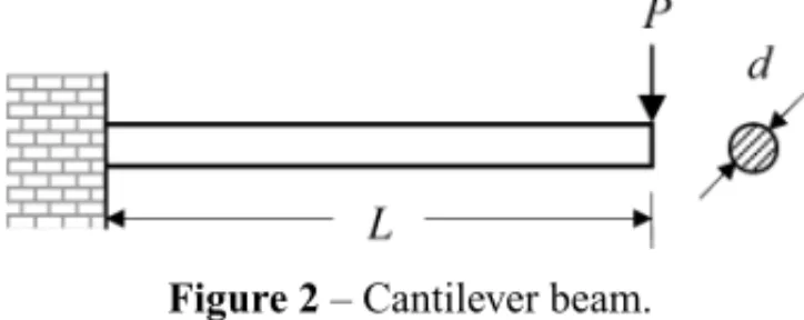
5.2 Design of a cantilever beam
As a second illustrative example, consider the design problem of a cantilever beam, adapted from Deb (2001). The beam, prismatic and with a circular section, must support the weightPat its free end. The design variables ared andL, the cross section diameter and beam length, respectively. Also consider two attributes to be minimized, the beam mass and the beam tip deflection when subjected to the weightP. Moreover, the maximum bending stress must be below of the material yield stress,σy, and the maximum tip displacement limited toδmax. A schematic representation
of the problem is shown in Figure 2.
Figure 2– Cantilever beam.
It can be demonstrated that the two selected objectives conflict since the minimization of the mass will lead to lower values of the pair(d,L)and minimization of the tip deflection will result in an increase in the cross sectional diameter with a reduction in the beam length.
The multi-objective optimization problem can be formulated as:
minimize tip deflection: δ(d,L)=64P L3/(3πEd4) (19a)
minimize beam mass: m(d,L)=0.25πρd2L (19b)
subjected to: 200≤L(mm)≤1000 (19c)
10≤d(mm)≤50 (19d)
δ(d,L)≤dmax (19e)
σ (d,L)=32P L/(πd3)≤σy (19f)
Adopting the following parameters:
P=1k N; δmax=5mm; σy =300M Pa; E =210G Pa; ρ=7850kg/m3
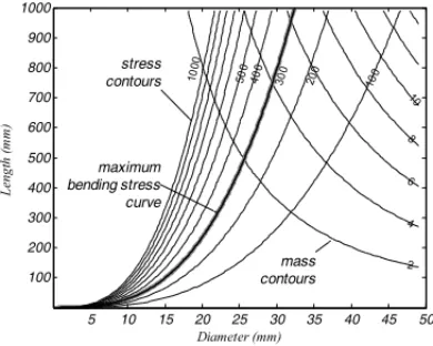
the shape of mass, tip deflection, and bending stress surfaces are shown in Figures (3a) and (3b).
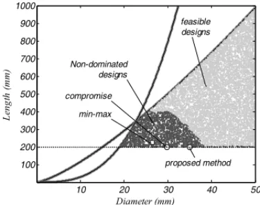
A clearer view of the antagonism of the objective functions can be obtained using a method to find the Pareto front of multi-objective optimization problems. Approximations of the Pareto set and the Pareto front and are shown in Figures (4a) and (4b), respectively. These results were found by generating 10,000 feasible designs at random and then selecting the non-dominated ones.
4 6 8 10 15 25 35 5 55 95 2 4 6 8 10 100 200 30
0 400 50
0 10
00
(a) Contours of the tip deflection and the beam mass.
(b) Contours of the bending stress and the beam mass.
Figure 3– Cantilever beam attributes.
relationship is observed considering the cross section diameter. Fixing the beam length, the lower the diameter the higher the tip deflection and the lower the beam mass.
Similar results were obtained by the NSGA II algorithm, using a 50 chromosomes population which has evolved 58 generations, conditioned by the stop criteria, Eq. (16), withtolf =0.001.
For comparison, Figures (4e) and (4f) show the results found by the weighted sum approach. Fifty random sets of weights were used to reduce the normalized mass and deflection beam functions to a single scale.
Now suppose that the problem must include the beam manufacturing cost and that it should be minimized. Additionally, suppose the cost function being defined by the function:
$(d,L)=100 "
d−30 50
2
+
d−30
50
L−400 1000
+
L−400 1000
2#
(20)
The contours of the cost function are shown in Figure (5a).
If the cost function is included as the third function in the MOOP, there is a growth and dispersion of Pareto optimal solutions in the design space, as shown in Figure (5b). This spread of the non-dominated alternatives in the design space makes decision making process even more difficult.
The proposed methodology can help the DM elect one alternative among all non-dominated, while preserving the concept of multi-objective optimization. The MOOP of the design of a cantilever beam can be re-formulated as:
Among all non-dominated design alternatives for the cantilever beam, where it is searched to minimize the beam tip deflection,δ(d,L), and minimize the beam mass, m(d,L), find the one that has the minimum manufacturing cost.
(a) Feasible and non-dominated designs for the cantilever beam in the design space.
(b) Feasible and non-dominated designs for the cantilever beam in the criterion space.
(c) Pareto set of the MOOP involving the beam mass and tip deflection obtained by the
NSGA II algorithm.
(d) Pareto front of the MOOP involving the beam mass and tip deflection obtained by the
NSGA II algorithm.
(e) Pareto set of the MOOP involving the beam mass and tip deflection obtained by the
weighted sum approach.
(f) Pareto front of the MOOP involving the beam mass and tip deflection obtained by the
weighted sum approach.
0.5 2
4 6
8
(a) Feasible and non-dominated designs for the cantilever beam in the design space.
(b) Non-dominated designs, in the design space, considering cost as the third objective function.
(c) Non-dominated designs, in criterion space, considering cost as the third objective function.
(d) Cost of the non-dominated designs obtained by the random walk and ilustrated in Figure (4a).
Figure 5– Adding the cost function to the MOOP involving the design of a cantilever beam.
Applying the proposed methodology, the MOOP can be rewritten as:
findXextended = x1,x2, α1, α2, λ1∙ ∙ ∙λ6T
that
minimizes: $(d,L)=100 "
d−30 50
2
+
d−30
50
L−400 1000
+
L−400 1000
2# (21a)
subject to: α1∇δ+α2∇m+ 6
X
j=1
λj∇gj =0 (21b)
gj ≤0, j =1,2, . . . ,6 (21c)
λj ≥0 (21e)
αi ≥0; α1+α2=1 (21f)
g1=σ (d,L)−σy (21g)
g2=δ(d,L)−δmax (21h)
g3=10−d (21i)
g4=d−50 (21j)
g5=200−L (21k)
g6=L−1000 (21l)
The fmincon was used to solve this single-objective optimization problem, which returns the following values
(d,L) = 35.0077,200.0000
α = 0.8144 0.1856T
λ = 0.0000 0.0000 0.0000 0.0000 0.0035 0.0000T
Note that the design variables(d,L)and the weighting factors (onlyλ5is not zero, revealing that
only the constraint equationg5, Eq. (21k), is active) converged to a point on the Pareto optimal
set for the MOOP involving the performance functions only, as shown in Figure (4a). For the sake of illustration, the values of the manufacturing cost calculated over the Pareto set obtained for the bi-objective optimization problem are shown in Figure (5d). The minimum cost is located in the diameter axis at the neighborhood of 35 mm.
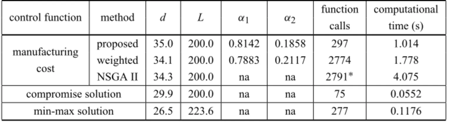
Table 2 shows a comparison of the methodologies used to find the single solution for the beam design. Although the proposed methodology does not return the Pareto front it is very efficient to find the final solution with number of function calls significantly smaller than the other two methods used for the same purpose.
Table 2– Results for the design optimization of a cantilever beam.
control function method d L α1 α2 function computational calls time (s) manufacturing proposed 35.0 200.0 0.8142 0.1858 297 1.014
cost weighted 34.1 200.0 0.7883 0.2117 2774 1.778 NSGA II 34.3 200.0 na na 2791∗ 4.075 compromise solution 29.9 200.0 na na 75 0.0552
min-max solution 26.5 223.6 na na 277 0.1176
∗58 generations completed.
over a surface, as shown in Figure (5b). In fact, the greater the number of conflicting functions in a multi-objective optimization problem, the greater the region in the space of the design variables that defines the Pareto optimal solutions. Consequently, the decision making process to elect a single solution is more difficult. How do we choose a non-dominated alternative among those present in Figure (5b)? The answer is impossible unless a fourth criterion is used to drive the choice. Rather, in the present proposal, this additional criterion is added to the MOOP as a control function to guide a convenient solution that satisfies all the constraints in a very efficient way, a solution that is non-dominated inside the group of the performance functions, and is an appropriate optimal solution obtained by optimizing the control function.
5.3 Conceptual design of a bulk carrier
The third application of the developed methodology was in the conceptual design of a bulk carrier. The conceptual design of a cargo vessel is not a trivial task. For decades, this problem has been handled in two ways, either by the adapting a known design aiming to the new requirements, or by the aid of simplified mathematical models driven by an optimization algorithm that enables obtaining the optimal solution based on technical or economic criteria previously established.
This work explores the second alternative with the help of the mathematical model for conceptual design of bulk carriers developed by Pratyush & Yang (1998) and presented in Appendix A. The model is made up of functions that define the vessel attributes from which are drawn those that constrain the design space, those to be optimized and those that characterize the technical and economic performance of the vessel and allow the evaluation of each design alternative. Among them are the annual transportation cost, the annual transported cargo, the ship lightweight, the ship initial costand other functions of the vessel design variables such as length, width, depth, draft, block coefficient and speed, respectively(L,B,D,h,CB,Vk). Pratyush & Yang (1998) proposed a general problem with explicit bounds on the block coefficient that should range between 0.63 and 0.75, and the ship speed that varies between 14 and 18 knots, and nine constraints in attributes, presented in Table A1 of Appendix A.
Parsons & Scott (2004) used the same model for comparing optimization methods, but they have altered the explicit bounds on the design variables. They limited the ship length at 274.32 m (900 ft) and the minimum deadweight at 25,000 ton, as shown in Table A2 of Appendix A. They also evaluated the problem by constraining the decision space in order to design ships suitable to cross the Panama Canal, with beam and draft limited to 32.31 m and 11.71 m, respectively, as shown in Table A3 of Appendix A.
Using Parsons and Scott’s second model, Hart & Vlahopoulou (2009) constrained the depth to the minimum and the maximum of 13 m and 25 m, respectively, and extended the acceptable range for ship speed to the values of 11 knots and 20 knots, minimum and maximum respectively, as shown in Table A4 of Appendix A.
may undermine not only the quality but even the validity of the results obtained by using the model. In this paper was used the constraint bounds on design variables proposed in Pratyush & Yang’s (1998) original work. For practical reasons, the limits they have not mentioned were adopted wide enough to not influence the optimization results. Accordingly, the ranges for the design variables are described in Table A5 of Appendix A.
5.3.1 Conflicting objectives
Pratyush & Yang (1998) chose to minimize theannual transportation cost, maximize the amount of annual transported cargo and minimize vessel lightweight. In this work, we replaced the vessel lightweight by the ship initial cost. Although vessel lightweight and ship initial cost
functions are related, the latter has a financial appeal like the former two objective functions.
Annual transported cargois associated with the annual income, theannual transportation cost
with the annual expenses and theship costis related to the capital required for the ship purchase.
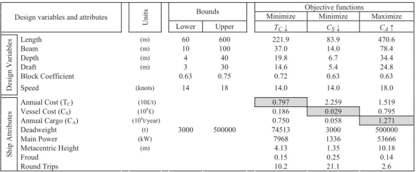
The design alternative that optimizes the single-objective problem can be easily obtained by taking each objective function separately. Any algorithm running with non-linear optimization problems and constraints can be used to solve this single-objective optimization problem. The
fminconwas used to get the results shown in Table 3.
Table 3– Results of the single-objective optimization of each objective function.
Objective functions Bounds
Minimize Minimize Maximize
Design variables and attributes
U
n
it
s
Lower Upper
Length (m) 60 600 221.9 83.9 470.6
Beam (m) 10 100 37.0 14.0 78.4
Depth (m) 4 40 19.8 6.7 34.4
Draft (m) 3 30 14.6 5.4 24.8
Block Coefficient 0.63 0.75 0.72 0.63 0.63
D es ig n V ar ia b le s
Speed (knots) 14 18 14.0 14.0 18.0
Annual Cost (TC) (10£/t) 0.797 2.259 1.519
Vessel Cost (CS) (10
8
£) 0.186 0.029 0.795
Annual Cargo (CA) (106t/year) 0.750 0.058 1.271
Deadweight (t) 3000 500000 74513 3000 500000
Main Power (kW) 7968 1336 53666
Metacentric Height (m) 4.13 1.35 10.18
Froud 0.15 0.25 0.14
S h ip A tt ri b u te s
Round Trips 10.2 21.1 2.6
Table 4– Statistics of the non-dominated solutions obtained by the random walk.
Design variables L B D T CB
Vk (m) (m) (m) (m) (knots) ˉ
xi 352.5 54.1 30.3 19.6 0.70 16.0 σi 75.4 11.6 6.6 4.1 0.03 1.2
xmin 88.4 13.6 6.4 5.1 0.63 14.0
xmax 493.5 77.1 40.0 26.3 0.75 18.0
Table 5– Statistics for the Pareto set obtained by the weighted sum approach.
Design variables L B D T CB
Vk
(m) (m) (m) (m) (knots) ˉ
xi 267.5 44.0 23.8 17.4 0.74 14.4 σi 82.2 13.7 7.4 5.1 0.03 0.8
xmin 94.2 15.7 7.6 6.0 0.63 14.0
xmax 425.5 68.9 36.6 26.3 0.75 18.0
5.3.2 Solutions for the MOOP
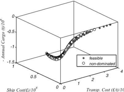
A clearer view of the antagonism of the objective functions in this problem can be obtained using an algorithm to find the Pareto front of multi-objective optimization problems. Figure 6 shows 10,000 feasible ship designs and highlights the non-dominated ones. To get these points, more than 12 million random design alternatives were generated and analyzed, taking 1097 seconds of computational time. Table 4 shows the design variables statistics for the feasible points. Al-though the problem shows a narrow surface in the criterion space, the design variables are well distributed over the design space.
With the aid of Figure 6, is possible to presume how the Pareto front of this problem should be, but, on the other hand, the random walk is not adequate to drive the search for the Pareto front, while the number of function calls becomes prohibitive.
In order to compare the results of the proposed methodology with other methods, the weighted sum approach and the genetic algorithm were used to do the bulk carrier design optimization task.
Figure 7 and Table 5 show the results of the weighted sum approach algorithm with 100 sets of random weights. Asfminconfails in find the solution for several weights sets, the process were restarted from 5 different starting points for each set single run, being chosen the best result as the resultant point. Even though points were discarded, because they have shown to be dominated solutions.
(a) Feasible and non-dominated designs for the bulk carrier obtained by a random walk in the design space.
(b)x-yview of the feasible and non-dominated designs.
(c)x-zview of the feasible and non-dominated designs.
(d)y-zview of the feasible and non-dominated designs.
Figure 6– Feasible and non-dominated designs for the MOOP with theannual transportation cost(CT) minimization, theship cost(CS)minimization and theannual cargo(CA)maximization, obtained by a random walk over the design variables.
The statistics for the design variables indicate a reasonable dispersion of the values. With the set of non-dominated solutions, shown in Figure 8, the question that often arises for the DM is:
which design alternative should be implemented?
5.3.3 Applying the proposed methodology
(a) Pareto front obtained by the weighted
sum approach. (b)x-yview of the Pareto front.
(c)x-zview of the Pareto front. (d)y-zview of the Pareto front.
Figure 7– Pareto front for the MOOP with theannual transportation cost(CT)minimization, theship cost (CS)minimization and theannual cargo(CA)maximization obtained by the weighted sum approach with 100 random weight sets.
among all the non-dominated solutions that would be obtained by resolving the MOOP for the bulk carrier design, namely, minimizing the annual transportation cost(CT), minimizing the ship cost(CS)and maximizing the annual cargo(CA),
find the solution that minimizes the voyage cost(CV).
(a) Pareto front for the bulk carrier design obtained
by the NSGA II algorithm. (b)x-yview of the Pareto front.
(c)x-zview of the Pareto front. (d)y-zview of the Pareto front.
Figure 8– Pareto front for the MOOP with theannual transportation cost(CT)minimization, theship cost (CS)minimization and theannual cargo(CA)maximization obtained by the NSGA II algorithm.
weighting factorsαkrelated to the gradients of the performance functions and more 21 weighting factorsλjrelated to the explicit and implicit constraints).
Table 7 shows the design alternative with some ship attributes obtained by using the fmincon
algorithm. Additionally, the solution is highlighted in Figure 9 over the Pareto front of perfor-mance functions obtained thanks to the NSGA II.
Table 8 compares the results obtained by the proposed methodology with those obtained by the weighted sum approach and the NSGA II. The proposed methodology is very efficient in finding the optimized design as the number the function calls is significantly smaller.
Table 6– Statistics for the Pareto set obtained by the NSGA II.
Design variables L B D T CB
Vk (m) (m) (m) (m) (knots) ˉ
xi 238.0 38.3 20.3 14.6 0.71 14.8 σi 113.5 18.7 10.1 7.0 0.05 1.1
xmin 84.2 14.0 6.4 5.0 0.63 14.0
xmax 443.1 70.2 38.3 26.3 0.75 18.0
Table 7– Results of the design optimization with the proposed methodology.
Table 8– Results for the design optimization of a bulk carrier.
method L,B,D,h CB V control function computational
(m) (knots) function (£) calls time (s) proposed 98.8, 12.8, 6.6, 5.2 0.63 14.0 12855 1031 7.872 weighted 94.2, 15.7, 7.6, 6.0 0.63 14.0 16466 69666 73.236 NSGA II 86.3, 13.5, 6.7, 5.4 0.64 14.0 13660 75783∗ 272.125 compromise 270.3, 45.1, 22.4, 16.4 0.64 14.0 na 239 0.206
min-max 258.8, 43.1, 23.5, 17.2 0.75 14.0 na 519 0.474
∗797 generations completed.
6 CONCLUSION
Most engineering design problems are multi-objective and the cases where the objective func-tions do not conflict are rare. To solve these kinds of problems, many researchers developed methods to search for the solution of multi-objective optimization without simplifying the prob-lem to single-objective and having to decidea priorihow to group the objective functions into a single scale. The evolutionary methods are frequently used to locate the set of solutions of multi-objective problems. These algorithms provide a discrete picture of the Pareto front in the criterion space. It was observed that the greater the number of objective functions, the more scattered the set of non-dominated solutions is in the decision space and the harder it is for the DM to choose an alternative to be deployed.
(a) Solution for the bulk carrier design obtained by the proposed methodology.
(b)x-yview of Pareto front of the bulk carrier design obtained by the NSGA II.
(c) Pareto front of the bulk carrier design obtained by the NSGA II.
(d) Pareto front of the bulk carrier design obtained by the NSGA II.
Figure 9– Pareto front obtained by the NSGA II for the MOOP involving the performance group{annual
transportation cost(CT),ship cost(CS), andannual cargo(CA)}and solution obtained by the proposed
methodology withvoyage cost(CV)as the control function.
group. Through this strategy, a single-objective optimization problem is formulated, in which the control function will be optimized over the Pareto set that would result from the optimization problem established by the performance functions, if this problem was previously solved.
Then the resultant single-objective optimization problem can be solved by any classical standard optimization engines, the limitations will be those present in the method used, such as the nature of the functions, whether they are linear or nonlinear, or continuous, regarding the presence or not of inequality and equality constraints.
With the proposed method a minimum knowledge is neededa priori. There is no need to know a value function relation to the objectives before starting to solve the problem as other a priori
As drawbacks, the method doesn’t provide a set of non-dominated solutions and as in many other single-objective optimization algorithms, the solution converges to a local optimum since the conditions of Karush-Kuhn-Tucker, chief pillar of the proposed methodology, are the necessary conditions but not sufficient to ensure that the solution is in the “global” Pareto front. If the problem is convex and the functions involved are regular, the local solution also will be a global solution, ensuring a unique result for the problem. Another disadvantage, the functions involved in the problem shall be continuously differentiable.
Although these conditions are limiting, the proposed methodology is very efficient in solving engineering design problems, as demonstrated by the examples solved with its use.
REFERENCES
[1] BOUYERE, CAROS, CHABLATD & ANGELES, J. 2007. The Multiobjective Optimization of a
Prismatic Drive, in Proceedings of ASME Design Engineering Technical Conferences, September
4-7, Las Vegas, Nevada, U.S.
[2] CHARNESA & COOPERWW. 1977. Goal programming and multiple objective optimisation – Part
1.European Journal of Operational Research,1: 39–54.
[3] CHINCHULUUN A & PARDALOS PM. 2007. A survey of recent developments in multiobjective optimization.Ann. Oper. Res.,154: 29–50.
[4] COELLO CAC. 2000. An Updated Survey of GA-Based Multiobjective Optimization Techniques.
ACM Computing Surveys(CSUR),32(2).
[5] COELLO CAC. 2010. List of References on Evolutionary Multiobjective Optimization, in URL <http://www.lania.mx/∼ccoello/EMOO/EMOObib.html>, April 24, 2010.
[6] DEBK, AGRAWALS, PRATABA & MEYARIVAN T. 2000.A Fast Elitist Non-Dominated Sorting
Genetic Algorithm for Multi-Objective Optimization, NSGA, KanGAL report 200001.
[7] DEB K. 2001.Multi-objective Objective Optimization using Evolutionary Algorithms, Wiley and Sons Ltd.
[8] EDGEWORTH FY. 1881.Mathematical Psychic: an essay on the application of mathematics to the
moral sciences, Editor P. Kegan, London, England.
[9] GIASSI A, BENNIS F & MAISONNEUVE JJ. 2004. Multi-Objective Optimization Using Asyn-chronous Distributed Applications.J. Mech. Des.,26: 767.
[10] GOLDBERG D. 1989. Genetic Algorithms in Search and Machine Learning, Reading, Addison Wesley.
[11] HAIMESYY, LASDONLS & WISMERDA. 1971. On a bicriterion formulation of the problems of integrated system identification and system optimization.IEEE Trans. Syst. Man Cybern. SMC-1, 296–297.
[12] HARTCG & VLAHOPOULOSN. 2009.An Integrated Multidisciplinary Particle Swarm Optimization
Approach to Conceptual Ship Design, Struct. Multidisc. Optim. DOI 10.1007/s00158-009-0414-0.
Springer-Verlag.