BGD
12, 7979–8034, 2015Linking ecosystem fluxes to canopy phenology in Europe
L. Wingate et al.
Title Page
Abstract Introduction
Conclusions References
Tables Figures
◭ ◮
◭ ◮
Back Close
Full Screen / Esc
Printer-friendly Version
Interactive Discussion
Discussion
P
a
per
|
Discussion
P
a
per
|
Discussion
P
a
per
|
Discussion
P
a
per
|
Biogeosciences Discuss., 12, 7979–8034, 2015 www.biogeosciences-discuss.net/12/7979/2015/ doi:10.5194/bgd-12-7979-2015
© Author(s) 2015. CC Attribution 3.0 License.
This discussion paper is/has been under review for the journal Biogeosciences (BG). Please refer to the corresponding final paper in BG if available.
Interpreting canopy development and
physiology using the EUROPhen camera
network at flux sites
L. Wingate1, J. Ogée1, E. Cremonese2, G. Filippa2, T. Mizunuma3,
M. Migliavacca4, C. Moisy1, M. Wilkinson5, C. Moureaux6, G. Wohlfahrt7,29,
A. Hammerle7, L. Hörtnagl7,15, C. Gimeno8, A. Porcar-Castell9, M. Galvagno2,
T. Nakaji10, J. Morison5, O. Kolle4, A. Knohl11, W. Kutsch12, P. Kolari9,
E. Nikinmaa9, A. Ibrom13, B. Gielen14, W. Eugster15, M. Balzarolo14,16,
D. Papale16, K. Klumpp17, B. Köstner18, T. Grünwald18, R. Joffre19,
J.-M. Ourcival19, M. Hellstrom20, A. Lindroth20, G. Charles21, B. Longdoz22,
B. Genty23,24, J. Levula9, B. Heinesch6, M. Sprintsin25, D. Yakir26, T. Manise6,
D. Guyon1, H. Ahrends15,27, A. Plaza-Aguilar28, J. H. Guan4, and J. Grace3
1
INRA, UMR ISPA 1391, 33140 Villenave d’Ornon, France
2
Environmental Protection Agency of Aosta Valley, ARPA Valle d’Aosta, Climate Change Unit, Italy
3
School of GeoSciences, University of Edinburgh, Edinburgh, EH9 3JN, UK
4
Max Planck Institute for Biogeochemistry, Jena, Germany
5
BGD
12, 7979–8034, 2015Linking ecosystem fluxes to canopy phenology in Europe
L. Wingate et al.
Title Page
Abstract Introduction
Conclusions References
Tables Figures
◭ ◮
◭ ◮
Back Close
Full Screen / Esc
Printer-friendly Version
Interactive Discussion
Discussion
P
a
per
|
Discussion
P
a
per
|
Discussion
P
a
per
|
Discussion
P
a
per
6
Unite de Physique des Biosystemes, Gembloux Agro-Bio Tech, Université of Liège, 5030 Gembloux, Belgium
7
University of Innsbruck, Innsbruck, Austria
8
Centro de Estudios Ambientales del Mediterráneo, Paterna, Spain
9
Department of Forest Sciences, University of Helsinki, P.O. Box 27, 00014, Finland
10
University of Hokkaido, Hokkaido, Japan
11
Georg-August University of Göttingen, 37077 Göttingen, Germany
12
Johann Heinrich von Thünen-Institut (vTI) Institut für Agrarrelevante Klimaforschung, 38116 Braunschweig, Germany
13
Risø National Laboratory for Sustainable Energy, Risø DTU, 4000 Roskilde, Denmark
14
Department of Biology/Centre of Excellence PLECO, University of Antwerp, Antwerp, Belgium
15
ETH Zurich, Institute of Agricultural Sciences, 8092 Zurich, Switzerland
16
Department of Forest Environment and Resources, University of Tuscia, Viterbo, Italy
17
INRA, Grassland Ecosystem Research Unit, UR874, 63100 Clermont Ferrand, France
18
Chair of Meterorology, Technische Universität Dresden, Tharandt, Germany
19
CNRS, CEFE (UMR5175), Montpelier, France
20
Department of Physical Geography and Ecosystem Science, Lund University, 22362 Lund, Sweden
21
Centre for Ecology and Hydrology, Wallingford, Oxford, UK
22
INRA, UMR EEF (UMR1137) Nancy, France
23
CEA, IBEB, SVBME, Laboratoire d’Ecophysiologie Moléculaire des Plantes, 13108 Saint-Paul-lez-Durance, France
24
CNRS, UMR Biologie Végétale et Microbiologie Environnementales (UMR7265), 13108 Saint-Paul-lez-Durance, France
25
Israeli Forest Service, Israel
26
Weizmann Institute for Science, Rehovot, Israel
27
Institute for Geophysics and Meteorology, University of Cologne, 50674 Cologne, Germany
28
University of Cambridge, Cambridge, UK
29
BGD
12, 7979–8034, 2015Linking ecosystem fluxes to canopy phenology in Europe
L. Wingate et al.
Title Page
Abstract Introduction
Conclusions References
Tables Figures
◭ ◮
◭ ◮
Back Close
Full Screen / Esc
Printer-friendly Version
Interactive Discussion
Discussion
P
a
per
|
Discussion
P
a
per
|
Discussion
P
a
per
|
Discussion
P
a
per
|
Received: 27 February 2015 – Accepted: 23 April 2015 – Published: 27 May 2015
Correspondence to: L. Wingate ([email protected])
BGD
12, 7979–8034, 2015Linking ecosystem fluxes to canopy phenology in Europe
L. Wingate et al.
Title Page
Abstract Introduction
Conclusions References
Tables Figures
◭ ◮
◭ ◮
Back Close
Full Screen / Esc
Printer-friendly Version
Interactive Discussion
Discussion
P
a
per
|
Discussion
P
a
per
|
Discussion
P
a
per
|
Discussion
P
a
per
Abstract
Plant phenological development is orchestrated through subtle changes in photope-riod, temperature, soil moisture and nutrient availability. Presently, the exact timing of plant development stages and their response to climate and management practices are crudely represented in land surface models. As visual observations of phenology
5
are laborious, there is a need to supplement long-term observations with automated techniques such as those provided by digital repeat photography at high temporal and spatial resolution. We present the first synthesis from a growing observational network of digital cameras installed on towers across Europe above deciduous and evergreen forests, grasslands and croplands, where vegetation and atmosphere CO2 fluxes are
10
measured continuously. Using colour indices from digital images and using piecewise regression analysis of time-series, we explored whether key changes in canopy phe-nology could be detected automatically across different land use types in the network. The piecewise regression approach could capture the start and end of the growing season, in addition to identifying striking changes in colour signals caused by
flow-15
ering and management practices such as mowing. Exploring the dates of green up and senescence of deciduous forests extracted by the piecewise regression approach against dates estimated from visual observations we found that these phenological events could be detected adequately (RMSE<8 and 11 days for leaf out and leaf fall respectively). We also investigated whether the seasonal patterns of red, green and
20
blue colour fractions derived from digital images could be modelled mechanistically us-ing the PROSAIL model parameterised with information of seasonal changes in canopy leaf area and leaf chlorophyll and carotenoid concentrations. From a model sensitivity analysis we found that variations in colour fractions, and in particular the late spring “green hump” observed repeatedly in deciduous broadleaf canopies across the
net-25
BGD
12, 7979–8034, 2015Linking ecosystem fluxes to canopy phenology in Europe
L. Wingate et al.
Title Page
Abstract Introduction
Conclusions References
Tables Figures
◭ ◮
◭ ◮
Back Close
Full Screen / Esc
Printer-friendly Version
Interactive Discussion
Discussion
P
a
per
|
Discussion
P
a
per
|
Discussion
P
a
per
|
Discussion
P
a
per
|
ecosystems across Europe. Coupling such quasi-continuous digital records of canopy colours with co-located CO2flux measurements will improve our understanding of how
changes in growing season length are likely to shape the capacity of European ecosys-tems to sequester CO2in the future.
1 Introduction
5
Within Europe continuous flux measurements of CO2, water and energy exchange
be-tween ecosystems and the atmosphere started in the early 1990s at a handful of forest sites (Janssens et al., 2001; Valentini et al., 2000). Nowadays, through the realisation of large European programmes such as EUROFLUX and CARBOEUROPE-IP amongst others, the number of natural and managed terrestrial ecosystems where the
dynam-10
ics of water and CO2 fluxes are monitored continuously has increased tremendously
(Baldocchi, 2014; Baldocchi et al., 2001), and that number is set to be maintained in Europe for at least the next twenty years as part of the European Integrated Carbon Ob-servation System (ICOS, www.icos-infrastructure.eu/). This long-standing co-ordinated European network, placed across several important biomes, has already documented
15
dramatic inter-annual variability in the amount of CO2 sequestered over the growing season (Delpierre et al., 2009b; Le Maire et al., 2010; Osborne et al., 2010; Wu et al., 2012) and witnessed both the short-lived and long-term impacts of disturbance (Kowal-ski et al., 2004), heat waves (Ciais et al., 2005) and management practices (Kutsch et al., 2010; Magnani et al., 2007; Soussana et al., 2007) on the carbon and water
bal-20
ance of terrestrial ecosystems. As a direct result of such an observational network, it is now possible to estimate with greater confidence how evapotranspiration (ET) and net ecosystem CO2 exchange (NEE) have responded to changes in climate over recent years (Beer et al., 2010; Jung et al., 2010) and better constrain our predictions of how ecosystems are likely to respond in the future to changes in climate using land surface
25
BGD
12, 7979–8034, 2015Linking ecosystem fluxes to canopy phenology in Europe
L. Wingate et al.
Title Page
Abstract Introduction
Conclusions References
Tables Figures
◭ ◮
◭ ◮
Back Close
Full Screen / Esc
Printer-friendly Version
Interactive Discussion
Discussion
P
a
per
|
Discussion
P
a
per
|
Discussion
P
a
per
|
Discussion
P
a
per
The growth of new leaves every year is clearly signalled in atmospheric CO2 con-centration records and exerts a strong control on both spatial and temporal patterns of carbon (C) sequestration and water cycling (Keeling et al., 1996; Piao et al., 2008). Hence, for the purpose of understanding patterns and processes controlling C and wa-ter budgets across a broad range of scales, there are obvious advantages in creating
5
explicit links between flux monitoring, phenological observation and biogeochemical studies (Ahrends et al., 2009; Baldocchi et al.,2005; Kljun, 2006; Lawrence and Slingo, 2004; Richardson et al., 2007; Wingate et al., 2008). Leaf phenology has fascinated human observers for centuries and is related to external signals such as temperature or photoperiod (Aono and Kazui, 2008; Demarée and Rutishauser, 2009; Linkosalo
10
et al., 2009). In the modern era, phenology has gained a new impetus, as people re-alised that such records must be sustained over many years to reveal subtle changes in plant phenology in response to climate change (Rosenzweig et al., 2007) and im-prove our understanding of the abiotic but also biotic (metabolic and genetic) triggers that determine seasonal changes in plant development. Currently, descriptions of
phe-15
nology in dynamic vegetation models are poor and need to be improved and tested against long-term field observations if we are to predict the impact of climate change on ecosystem function and CO2 sequestration (Keenan et al., 2014b; Kucharik et al.,
2006; Richardson et al., 2011).
Variations in the concentrations of pigments and spectral properties of leaves also
20
provide a valuable mechanistic link to changes in plant development and photosyn-thetic rates when interpreted with models such as PROSAIL that combine our knowl-edge of radiative transfer through forest canopies and leaf mesophyll cells with leaf biochemistry (Jacquemoud and Baret, 1990; Jacquemoud et al., 2009). Automated techniques to detect and assimilate changes in the optical signals of leaves either near
25
BGD
12, 7979–8034, 2015Linking ecosystem fluxes to canopy phenology in Europe
L. Wingate et al.
Title Page
Abstract Introduction
Conclusions References
Tables Figures
◭ ◮
◭ ◮
Back Close
Full Screen / Esc
Printer-friendly Version
Interactive Discussion
Discussion
P
a
per
|
Discussion
P
a
per
|
Discussion
P
a
per
|
Discussion
P
a
per
|
This paper aims to synthesise data from flux sites across Europe where researchers have embraced the opportunity to establish automatic observations of phenological events by mounting digital cameras and recording daily (or even hourly) images of the vegetation throughout the seasons. We examine whether coherent seasonal changes in digital image properties can be observed at the majority of sites even if camera
5
types and configuration are not yet harmonised and calibration procedures are not fully developed. In this work we asked the following questions (i) how well can digital images be automatically processed to reveal the key phenological events such as leaf out, flowering, leaf fall, or land management practices such as mowing and harvesting; and (ii) can we provide a mechanistic link between digital images, leaf phenology and the
10
physiological performance of leaves in the canopy? To address the second question, we adapted the model PROSAIL (Jacquemoud and Baret, 1990; Jacquemoud et al., 2009) to simulate the seasonal changes in red, green and blue signals detected by digital cameras above canopies and performed sensitivity analysis of these signals to variations in canopy structure (leaf area, structure and angles) and biochemistry (leaf
15
pigment and water content).
2 Material and methods
2.1 Study sites and camera set-up
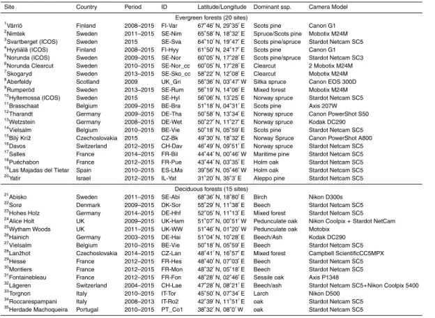
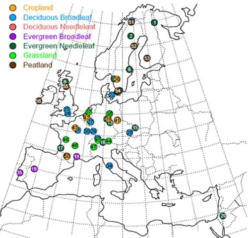
The European network of digital cameras currently covers over 50 flux sites across Europe (Fig. 1 and Table 1). Table 1 demonstrates that a diverse selection of
commer-20
cially available cameras are being used across the network. The cameras are installed in waterproof housing that is firmly attached to the flux tower some height above the top of the canopy. The cameras are generally orientated North, looking slightly down to the horizon to ensure that the majority of the image contains the vegetation of inter-est. Canopy images of the same scene are taken repeatedly each day, at a frequency
25
BGD
12, 7979–8034, 2015Linking ecosystem fluxes to canopy phenology in Europe
L. Wingate et al.
Title Page
Abstract Introduction
Conclusions References
Tables Figures
◭ ◮
◭ ◮
Back Close
Full Screen / Esc
Printer-friendly Version
Interactive Discussion
Discussion
P
a
per
|
Discussion
P
a
per
|
Discussion
P
a
per
|
Discussion
P
a
per
8 bit JPEG files (i.e. digital numbers ranging from 0 to 255). The archived images used in the present analysis are all taken between 11:00 and 13:00 LT. The camera setup is specific to each camera type but a common requirement to observe the seasonal colour fraction time-series is to set the colour balance to “fixed” mode (on the Star-dot cameras) or the white balance to “manual” mode (for the Nikon Coolpix cameras)
5
(Mizunuma et al., 2013, 2014).
2.2 Image analysis
2.2.1 ROI selection and colour analysis
For each site, a squared region of interest (ROI) was selected from visual inspection of the images. The ROI had to be as large as possible and common to all images of
10
the same growing season while including as many plants as possible but no soil or sky areas. Automated segmentation methods could also be used to select ROI with more complex geometries only on plant parts (e.g. Comar et al., 2012). However this would result in different ROI between images, that would be problematic for defining seasonal changes in image properties, and would also be somewhat impractical for
15
large datasets as it would require an a posteriori check for the success of the method on each image.
Image ROIs were then analysed using the open-source image analysis software, Image-J (Image-J v1.36b; NIH, MS, USA). A customised macro was used to extract Red-Green-Blue (RGB) digital number (DN) values between 0 and 255 (ncolour) for
20
each pixel of the ROI and a mean value for all pixel values in a given ROI of each image was calculated. Various colour indices can be obtained from digital image properties (Mizunuma et al., 2011), but here we used only the chromatic coordinates, called colour fraction hereafter (Richardson et al., 2007):
Colour Fraction =ncolour/(nred+ngreen+nblue) (1)
25
BGD
12, 7979–8034, 2015Linking ecosystem fluxes to canopy phenology in Europe
L. Wingate et al.
Title Page
Abstract Introduction
Conclusions References
Tables Figures
◭ ◮
◭ ◮
Back Close
Full Screen / Esc
Printer-friendly Version
Interactive Discussion
Discussion
P
a
per
|
Discussion
P
a
per
|
Discussion
P
a
per
|
Discussion
P
a
per
|
In the following we will thus refer to the “green fraction” as the mean green colour fraction for all pixels in the ROI, as opposed to the amount of pixels covered by vege-tation in the entire image (Comar et al., 2012).
2.2.2 Data filtering procedure
Image quality is often adversely affected by rain, snow, low clouds, aerosols, fog and
5
uneven patterns of illumination caused by the presence of scattered clouds. These influences often create noise in the trajectories of colour indices, and is an important source of uncertainty that can hamper the description of canopy seasonal variations and the derivation of robust phenological metrics from colour index time-series. To remove problematic images that were affected by raindrops, snow or fog from the digital
10
photograph analysis, we used a filtering algorithm based on the statistical properties of the time series, we used two steps to filter the raw data. The first filter, based on the deviation from a smoothed spline fit as described in Migliavacca et al. (2011), was used to remove outliers. Thereafter, we applied the method implemented in Sonnentag et al. (2012), to reduce the variability of the colour fractions (Fig. 2).
15
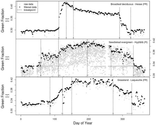
2.2.3 Piecewise break point change analysis
We used a piecewise break point regression approach to extract automatically the main phenological events such as leaf emergence and senescence from the colour fraction time series (Fig. 2). The procedure is implemented in the R package
struc-change(Zeileis et al., 2002, 2003) and is used to detect breaks in a time series by
20
identifying points where the multiple linear correlation coefficients shift from one stable regression relationship to another (Bai and Perron, 2003). The 95 % confidence inter-vals of the identified break points were then computed using the distribution function proposed by Bai (1997). To obtain credible breakpoints in complex green fraction time series such as in highly managed sites (e.g. grazed or cut grasslands, multiple rotation
25
BGD
12, 7979–8034, 2015Linking ecosystem fluxes to canopy phenology in Europe
L. Wingate et al.
Title Page
Abstract Introduction
Conclusions References
Tables Figures
◭ ◮
◭ ◮
Back Close
Full Screen / Esc
Printer-friendly Version
Interactive Discussion
Discussion
P
a
per
|
Discussion
P
a
per
|
Discussion
P
a
per
|
Discussion
P
a
per
may be necessary. However, such a high number of break points would be excessive in natural ecosystems, and so we decided to set a maximum of five breakpoints per growing season, for both managed and natural ecosystems. We opted for a breakpoint approach over other commonly used methods to extract phenological transitions from time series (i.e thresholds, derivative methods) because it can be considered as more
5
robust and less affected by noise in the time series (Henneken et al., 2013). This is particularly relevant for our application that encompasses a large dataset consisting of many different camera set-ups (camera type, target distance, image processing).
2.2.4 Determining phenophases by visual assessment
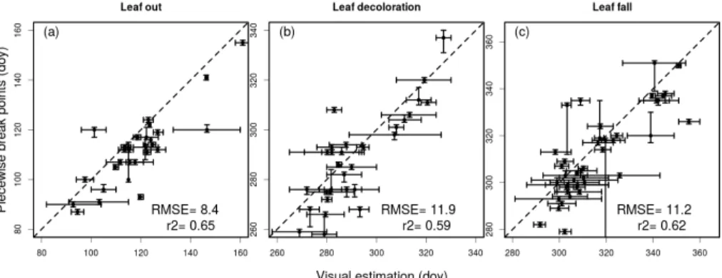
In order to relate the break point detection method to phenological phases we also
vi-10
sually examined images from broadleaf forest ecosystems for leafing out, senescence and leaf fall. Six pre-trained observers looked through the same daily images and used a common protocol to identify dates when (1) the majority of vegetation started leafing out (i.e. when 50 % of the ROI contains green leaves), (2) the canopy first started to change colour to (first non-green colours such as yellow and orange) in autumn and
15
(3) the last day when a few non-green leaves were still visible on the canopy before the day the branches became bare. These visually assessed dates were then aver-aged across observers and compared to the relevant breakpoints identifying the same phenological stage. The leafing out phase was associated to the first automatically de-tected breakpoint, leaf senescence to the penultimate breakpoint and leaf fall to the
20
last breakpoint. Based on this classification the key dates identified by the algorithm and visual inspection were consistently correlated with one another (Fig. 3). However, there was a tendency for the automatic algorithm to identify all the phenological tran-sitions before the visually assessed dates, by about a week. Also, visual inspections had larger standard deviations, especially during canopy senescence. Because of this
25
BGD
12, 7979–8034, 2015Linking ecosystem fluxes to canopy phenology in Europe
L. Wingate et al.
Title Page
Abstract Introduction
Conclusions References
Tables Figures
◭ ◮
◭ ◮
Back Close
Full Screen / Esc
Printer-friendly Version
Interactive Discussion
Discussion
P
a
per
|
Discussion
P
a
per
|
Discussion
P
a
per
|
Discussion
P
a
per
|
15.9 and 13.3 days respectively). These RMSE values fall, however, within the range recently found by Klosterman et al. (2014) in a similar validation exercise performed with data from various US deciduous forests.
2.3 Radiative transfer modelling
To interpret mechanistically the colour fraction time-series produced by cameras in the
5
network, we combined the bi-directional radiative transfer model PROSAIL (Jacque-moud and Baret, 1990; Jacque(Jacque-moud et al., 2009) with some basic spectral prop-erties of the photodetectors and the transmittances of the optical elements and fil-ters used in the cameras, all combined into the so-called spectral efficiency of the RGB color channels (GRGB, in DN W−
1
, defined as the digital number per watt).
Ex-10
amples of these properties are shown in the Supplement (Figs. S1 and S2) for two types of camera from the network: (1) the Stardot NetCam CS5, in use at the ma-jority of the European sites (Table 1) and the dominant camera used in the North American Phenocam network (http://phenocam.sr.unh.edu/webcam/) (Toomey et al., 2015) and (2) the Nikon Coolpix 4500, in use at two sites within the European
cam-15
era network, and ca. 17 sites within the Japanese Phenological Eyes Network (PEN) (http://pen.agbi.tsukuba.ac.jp/index_e.html) (Nasahara and Nagai, 2015).
The PROSAIL model combines the leaf biochemical model PROSPECT (PROSPECT-5) that simulates the directional-hemispherical reflectance and transmit-tance of leaves over the solar spectrum from 400 to 2500 nm (Jacquemoud and Baret,
20
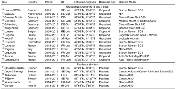
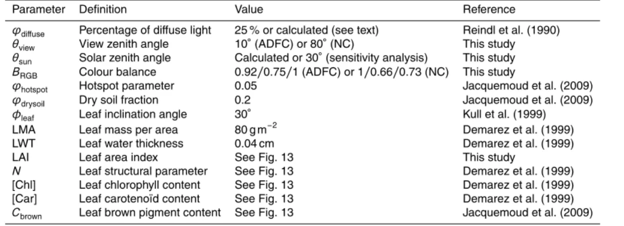
1990) and the radiative-transfer model SAIL (4SAIL (Verhoef, 1984)). The version of the model used here (version 5B for IDL http://teledetection.ipgp.jussieu.fr/prosail/) re-quires 11 parameters from PROSAIL (leaf area, leaf angle, leaf mass and chlorophyll, carotenoid, water or brown pigment contents, hotspot parameter, leaf structural pa-rameter and dry soil fraction, percentage of diffuse light) as well as geometrical
pa-25
rameters (sun height, view zenith angle and sun-view azimuthal difference angle). The percentage of diffuse light (ϕdiffuse) is necessary to calculate the amount of direct and
BGD
12, 7979–8034, 2015Linking ecosystem fluxes to canopy phenology in Europe
L. Wingate et al.
Title Page
Abstract Introduction
Conclusions References
Tables Figures
◭ ◮
◭ ◮
Back Close
Full Screen / Esc
Printer-friendly Version
Interactive Discussion
Discussion
P
a
per
|
Discussion
P
a
per
|
Discussion
P
a
per
|
Discussion
P
a
per
observed incoming global radiation (Rg, in W m− 2
) using a procedure developed by Reindl et al. (1990). The incoming radiation spectra at the top of the canopy are then estimated fromRg,ϕdiffuse, and mean, normalised spectra for direct (Idirect) and diffuse
(Idiffuse) radiation derived by Francois et al. (2002) using the 6S atmospheric radiative
transfer model (Fig. S3). The 6S simulations performed by François et al. considered
5
a variety of aerosol optical thicknesses at 550 nm (corresponding to a visibility rang-ing from 8.5 to 47.7 km), water vapor content (from 0.5 to 3.5 g cm−2, corresponding to most situations encountered in mid-latitudes), solar incident angle (from 0 to 78.5◦) and standard values for ozone, CO2 and other atmospheric constituents but did not consider the presence of clouds. Therefore the derived spectra are only valid for
cloud-10
free conditions and, following Francois et al. (2002), values ofϕdiffuse below 0.5 were
considered to represent such cloud-free sky conditions. PROSAIL was then used to estimate the amount of light reflected by the canopy in the direction of the camera for each wavelengthE(λ) (W m−2nm−1) from which we compute the RGB signals accord-ing to:
15
IRGB=BRGB
λZIR
λUV
GRGB(λ)E(λ)dλ (2)
whereλUVandλIRare the UV and IR cut-offwavelengths of the camera sensor and
fil-ter (see Fig. S1) andBRGBis a constant factor that accounts for camera settings (mostly
colour balance) and was manually adjusted for each RGB signal and each camera/site using a few days of measurements outside the growing season. The modelled RGB
20
color fractions were then computed in a similar fashion as in Eq. 1 but withIRGBinstead
ofncolour. In practice, GRBG is often normalised to its maximum value rather than ex-pressed in absolute units and for this reasonIRGB is not a true digital number, but this
has no consequence once expressed in colour fractions. Also, we are aware that the image processing of real (non-uniform) scenes is far more complex than Eq. (2) (Farrell
25
BGD
12, 7979–8034, 2015Linking ecosystem fluxes to canopy phenology in Europe
L. Wingate et al.
Title Page
Abstract Introduction
Conclusions References
Tables Figures
◭ ◮
◭ ◮
Back Close
Full Screen / Esc
Printer-friendly Version
Interactive Discussion
Discussion
P
a
per
|
Discussion
P
a
per
|
Discussion
P
a
per
|
Discussion
P
a
per
|
seems robust enough to describe time-series of average colour fractions over a large and fixed ROI, measured with different camera settings.
2.4 CO2flux analysis
A recent study by Toomey et al. (2015) demonstrated that the seasonal variability in daily green fraction measured at 18 different flux sites generally correlated well with
5
GPP estimated from co-located flux towers over the season. However, they found that the correlation between daily GPP and daily green fraction was better for some plant functional groups (grasslands) than for others (evergreen needleleaf forests or decidu-ous broadleaf forests). Thus for some of the flux sites presented in Table 1, we also tried to relate, at least qualitatively, changes in vegetation indices to gross primary
produc-10
tivity (GPP) time-series. Net CO2fluxes were continuously measured at each site using the eddy covariance technique described in Aubinet et al. (2012). Level 4 datasets were both quality-checked and gap-filled using online eddy-covariance gap-filling and flux-partitioning tools provided by the European flux database cluster (Lasslop et al., 2010; Reichstein et al., 2005). Full descriptions of the flux tower set-ups used to compare
15
digital images and GPP are provided in Wilkinson et al. (2012) for Alice Holt (decidu-ous forest), Wohlfahrt et al. (2008) and Galvagno et al. (2013) for Neustift and Torgnon (sub-alpine grasslands), Vesala et al. (2010) for Hyytiälä (evergreen forest) and Aubinet et al. (2009) for Lonzee (cropland).
3 Results and discussion
20
3.1 Seasonal changes in green fraction across the network
3.1.1 Needleleaf forest ecosystems
BGD
12, 7979–8034, 2015Linking ecosystem fluxes to canopy phenology in Europe
L. Wingate et al.
Title Page
Abstract Introduction
Conclusions References
Tables Figures
◭ ◮
◭ ◮
Back Close
Full Screen / Esc
Printer-friendly Version
Interactive Discussion
Discussion
P
a
per
|
Discussion
P
a
per
|
Discussion
P
a
per
|
Discussion
P
a
per
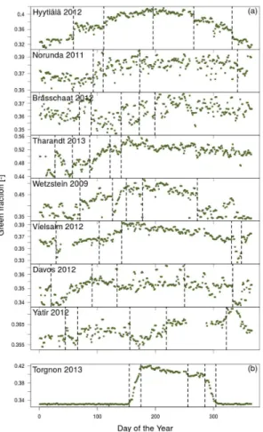
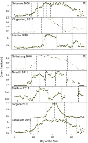
of approximately ca. 30◦(31◦20′N–61◦50′N) (Fig. 4 and Table 1). It was often difficult to automatically determine the start of the growing season for the coniferous sites, either because of snow cover (noticeable changes in the colour signals were often associ-ated with the beginning and end of snow cover) or because of problems caused by the set-up of the camera (either too far away from the crown or containing too much sky).
5
However seasonal changes in the amplitude of the canopy green fraction of needle-leaf trees were generally conservative across sites and often displayed a gentle rise in green fraction values during the spring months (Fig. 4a) and a gentle decrease during the winter months. In contrast, the deciduous Larix site in Italy showed a steep and pronounced start and end to the growing season that lasted approximately five months
10
(Fig. 4b).
The main evergreen conifer speciesPinus sylvestrisL. andPicea abiesL. tended to exhibit different green fraction variations during spring. InPicea species, new shoots contain very bright, light green needles that caused a noticeable increase in the green colour fraction during the months of May and June (Fig. 4, e.g. Tharandt and
Wet-15
zstein). In contrast, the new shoots of Pinus species primarily appeared light brown as the stem of the new shoot elongated (Fig. S4) and caused a small reduction in the green fraction, only detectable at a number of sites and years (Brasschaat in 2009, 2012; Norunda in 2011; Hyytiälä, 2008, 2009, 2010, 2012), followed by an increase in the green fraction values once needle growth dominated at the shoot scale (Figs. 4
20
and S4).
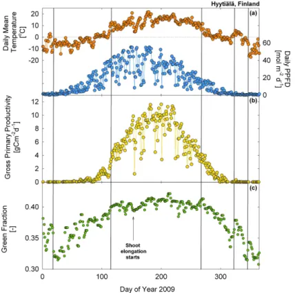
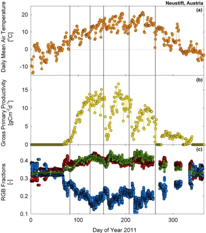
The breakpoint analysis could identify a change in the green fraction when the canopy became consistently snow-free or covered in snow, but also when it experi-enced sustained daily mean air temperatures of above 0◦C (Fig. 5). For instance, at the Finnish site Hyytiälä, the green fraction exhibited rapid changes during final snowmelt
25
(day 18, bp1) and first snowfall (day 346, bp5 confirmed with visual inspection of the images), but also around days 100–110 (bp2) as daily mean temperatures increased from−10◦C and stabilised for several days just above 0◦C and GPP rates increased
frac-BGD
12, 7979–8034, 2015Linking ecosystem fluxes to canopy phenology in Europe
L. Wingate et al.
Title Page
Abstract Introduction
Conclusions References
Tables Figures
◭ ◮
◭ ◮
Back Close
Full Screen / Esc
Printer-friendly Version
Interactive Discussion
Discussion
P
a
per
|
Discussion
P
a
per
|
Discussion
P
a
per
|
Discussion
P
a
per
|
tion were again detected by the piecewise regression approach, one around day 267 (bp3), coinciding with the period when minimum air temperatures began to fall below 0◦C and another around day 320 (bp4) coinciding with a short period of warmer tem-peratures (Fig. 5). Interestingly these breakpoints at the beginning (days 100–110, bp2) and the end (days 280–310, bp4) also coincided with the onset and cessation of GPP.
5
The recovery of biochemical reactions and the reorganisation of the photosynthetic ap-paratus in green needles is known to be triggered when air temperature rises above 0◦C (Ensminger et al., 2008, 2004) and at about 3–4◦C at this particular site in Finland (Porcar-Castell, 2011; Tanja et al., 2003). Our results suggest that green fractions from digital images seem sensitive enough to detect these changes in the organisation of
10
the photosynthetic apparatus of the coniferous evergreen needles.
3.1.2 Grassland and cropland ecosystems
Many land surface models still lack crop-related plant functional types and often sub-stitute cropland areas with the characteristics of grasslands (Osborne et al., 2007; Sus et al., 2010). Our initial results from the EUROPhen network demonstrate the difficulty
15
of teasing apart the seasonal and inter-annual developmental patterns as they are often complicated by co-occuring agricultural practices (e.g. cutting, ploughing, har-vesting and changes in animal stocking density) (Fig. 6).
Overall we found that there was surprisingly little difference between the onset dates of growth for most of the permanent grassland sites, despite being located in very
20
different locations across Europe. However the onset of the green fraction signal was considerably delayed at the sub-alpine grassland site in Torgnon compared with the other sites (Fig. 6). Torgnon also had the most compressed growing season of all the sites, encompassing a period of less than 100 days, some 100 days shorter than the other sites. These differences in growing season length between permanent grassland
25
sites are caused by elevation (most grassland sites are situated at 1000±50 m a.s.l.,
BGD
12, 7979–8034, 2015Linking ecosystem fluxes to canopy phenology in Europe
L. Wingate et al.
Title Page
Abstract Introduction
Conclusions References
Tables Figures
◭ ◮
◭ ◮
Back Close
Full Screen / Esc
Printer-friendly Version
Interactive Discussion
Discussion
P
a
per
|
Discussion
P
a
per
|
Discussion
P
a
per
|
Discussion
P
a
per
Management practices such as the cutting of meadows (e.g. Neustift and Früebüel) and changes in animal stocking rate (e.g. Laqueuille) also created abrupt shifts in the RGB signals that could be distinguished from digital images. For example at the Neustift site in Austria, the meadow was cut three times during the 2011 growing sea-son (days 157, 213, 272) causing pronounced drops in the blue fraction and to a lesser
5
extent reductions in the green and red signal (Fig. 7). These meadow cuts were clearly identified in the green fraction time-series by the breakpoint analysis (see bp3, bp4 and bp5 in Figs. 6 and 7). In addition, flowering events were frequently strong drivers of the colour signals at the Neustift site and led to gradual decreases in the red and green signals for several weeks prior to mowing (e.g. yellow flowers on days 134–156
10
(bp2), white flowers on days 176–212). In contrast the blue signal tended to increase in strength during flowering periods making the impact of the mowing events dramatic when they occurred (Fig. 7). If the piecewise regression algorithm was set to allow the detection of up to 8 breakpoints at those sites, flowering events were often identified as well as the mowing events but this made the detection of the start and end dates
15
of the growing season even more challenging using automated algorithms. Sometimes up to 8 breakpoints could be observed in grassland ecosystems and frequently the first breakpoint was caused by the start of the snow free period, as opposed to the start of growth. Subsequent breakpoints typically indicated the phenology and management of the vegetation, particularly mowing, and suggest a visual inspection of images may
20
still be necessary to clarify the nature and management causes behind breakpoints in some grassland sites.
In addition, at some sites it was not always easy to discern visually from images when a grassland started its first growth as often fresh shoots are hidden by litter and dead material from the previous year. This particular problem may lead to a slight
overesti-25
BGD
12, 7979–8034, 2015Linking ecosystem fluxes to canopy phenology in Europe
L. Wingate et al.
Title Page
Abstract Introduction
Conclusions References
Tables Figures
◭ ◮
◭ ◮
Back Close
Full Screen / Esc
Printer-friendly Version
Interactive Discussion
Discussion
P
a
per
|
Discussion
P
a
per
|
Discussion
P
a
per
|
Discussion
P
a
per
|
Given these preliminary results at Neustift, Torgnon and the other EUROPhen sites, it appears that grassland green signals may provide some information on the variations in GPP over the season and between years as suggested by Migliavacca et al., (Migli-avacca et al., 2011) and more recently Toomey et al. (2015) but an underestimation of the growing season length may also occur using our automatic breakpoint detection
5
approach.
As mentioned above, the use of grassland characteristics to describe the phenology of different crops is common in models. However, at the same site we can see that the start of the growth period for each different crop varies widely over commonly applied rotations. For example at Lonzee in Belgium we found that for individual crop types
10
such as potato and winter wheat the patterns of the green signal were fairly similar between different years (Fig. 9). However, we could still observe variations between years such as a slightly shorter green period for the potatoes in 2014 relative to 2010 or a slightly later start to the season for winter wheat in 2013 relative to 2011.
As huge areas of Europe are dedicated to the production of crops (326 Mha) and
15
grasslands (151 Mha) (Janssens et al., 2003) and are known to be one of the largest European sources of biospheric CO2 to the atmosphere at a rate of about 33Tg C y−1
(Schulze et al., 2009), it is increasingly important that more field observations of devel-opmental or phenological transitions are obtained to constrain the timing and develop-mental rate of plants in situ and improve model simulations. Our initial results from the
20
EUROPhen camera network show that digital repeat photography may provide a valu-able assimilation dataset in the future for constraining variations in the timing of LAI changes across rotations as well as providing useful indicators of developmental tran-sitions and agricultural practices (e.g. cutting, ploughing, harvesting and changes in animal stocking density).
25
3.1.3 Broadleaf forest ecosystems
sig-BGD
12, 7979–8034, 2015Linking ecosystem fluxes to canopy phenology in Europe
L. Wingate et al.
Title Page
Abstract Introduction
Conclusions References
Tables Figures
◭ ◮
◭ ◮
Back Close
Full Screen / Esc
Printer-friendly Version
Interactive Discussion
Discussion
P
a
per
|
Discussion
P
a
per
|
Discussion
P
a
per
|
Discussion
P
a
per
nals clearly across a range of broadleaf sites in the network it was necessary to show the seasonal patterns observed in different years across differnet sites mainly because there were often gaps in the images at one or more sites in each year. Despite Fig. 10 showing site data from different years, general patterns associated with broadleaf for-est characteristics were observed. Typically the start of the temperate growing season
5
coincides with a strong increase in the green signal and a decrease in the blue and red signals. Across the network the timing of this spring green-up varies slightly with latitude, usually occurring first in the southern sites and moving North with the British sites starting later than continental sites at similar latitudes (Fig. 10). The end of the growing season, identified clearly as a decrease in the green signal, varied
consider-10
ably across the network. The more continental sites such as the Hainich and Lägeren deciduous forests exhibited the shortest growing season lengths, whilst the oceanic and Mediterranean sites had far longer growing seasons. A high degree of variability in the timing for colour changes in autumn is expected across temperate deciduous ecosystems (Archetti et al., 2008) despite the fact that, at least in the case of European
15
tree species, changes in photoperiod and air temperature are usually considered the main drivers of the colouration of senescent leaves (Delpierre et al., 2009a; Keskitalo et al., 2005; Menzel et al., 2006).
Interestingly, the evergreen broadleaf forests at the Mediterranean sites displayed similar RGB seasonal variations (Fig. 10b). However, the peak in the green fraction
20
values were observed somewhat later in spring compared to those of the deciduous broadleaf sites. These maximum green fraction values are most probably linked to the production of new leaves that typically occurs at this period in Holm Oak (García-Mozo et al., 2007; La Mantia et al., 2003). Interestingly, a strong decrease in the green fraction was observed prior to the peak at the Spanish site, Majadas del Tieter.
Simi-25
BGD
12, 7979–8034, 2015Linking ecosystem fluxes to canopy phenology in Europe
L. Wingate et al.
Title Page
Abstract Introduction
Conclusions References
Tables Figures
◭ ◮
◭ ◮
Back Close
Full Screen / Esc
Printer-friendly Version
Interactive Discussion
Discussion
P
a
per
|
Discussion
P
a
per
|
Discussion
P
a
per
|
Discussion
P
a
per
|
photos (Fig. S5) we found that the canopy during this period was covered in conspicu-ous male catkin-type flowers that appear yellow-brown in the images (Fig. 10). These flowering events are critical for the production of acorns, that randomly alternate be-tween mast and low production years (Vázquez et al., 1990; Espárrago et al., 1992). Thus, in the case of the Spanish site at least, the strong decrease in the green
frac-5
tion seemed dominated by a male flowering event, in addition to the shedding of old leaves. In the case of the Puechabon site, visual inspection of the photos did not detect a strong flowering event, however, the camera is located slightly further away from the canopy making it difficult to detect flowers easily by eye. However, phenological records maintained at the site indicate that the period between bp2 and bp3 when the green
10
signal slightly decreases, coincides with the start and end of the male flowering period, as well as leaf fall. In contrast, the signal between bp3 and bp4 indicates the period of leaf flushing for this year. Further studies comparing NDVI signals with digital images should allow us to understand better the observed variations in both signals and their link to phenological events such as flowering and litterfall in evergreen broadleaves and
15
how these vary between years in response to climate.
For broadleaf deciduous (and to some extent evergreen) species our breakpoint ap-proach also detected a significant decline in the green fraction a few weeks after leaf emergence and well before leaf senescence (Figs. 2 and 10). This pattern in the green fraction has also been observed for a range of deciduous tree species in Asia and
20
the USA (Hufkens et al., 2012; Ide and Oguma, 2010; Keenan et al., 2014a; Nagai et al., 2011; Saitoh et al., 2012; Sonnentag et al., 2012; Toomey et al., 2015; Yang et al., 2014). In addition, this feature has also been observed at the leaf scale using scanned images of leaves (Keenan et al., 2014a; Yang et al., 2014) and at the regional scale for a number of deciduous forest sites using MODIS surface reflectance products
25
BGD
12, 7979–8034, 2015Linking ecosystem fluxes to canopy phenology in Europe
L. Wingate et al.
Title Page
Abstract Introduction
Conclusions References
Tables Figures
◭ ◮
◭ ◮
Back Close
Full Screen / Esc
Printer-friendly Version
Interactive Discussion
Discussion
P
a
per
|
Discussion
P
a
per
|
Discussion
P
a
per
|
Discussion
P
a
per
decline in the green fraction following budburst (Keenan et al., 2014a; Nagai et al., 2011). At two of the deciduous sites within our network, Alice Holt and Søro (Fig. 4), daily PAR transmittance was also measured providing a suitable proxy for changes in canopy leaf area. In both cases no decrease in the LAI proxy was detected during the decrease of the green signal shortly after budburst. If this decrease in the green signal
5
after leaf growth is not caused by a reduction in the amount of foliage in most cases, it is likely associated with either changes in the concentration and phasing of the different leaf pigments or changes in the leaf angle distribution. These different hypotheses are tested in the next section.
3.2 Modelling ecosystem RGB signals
10
3.2.1 Sensitivity analysis of model parameters
Using the PROSAIL model as described above, with the camera sensor specifications of the Alice Holt oak site (see Fig. S1) we performed three different sensitivity analy-ses of the simulated RGB fractions to the 13 model parameters (Table 2). All sensitivity analyses consisted of a Monte Carlo simulation of between 2000 and 10 000 runs each.
15
For the first analysis the model was allowed to freely explore different combinations of the parameter space over the range of values commonly found in the literature and with no constraints on how the parameters were related to each other (all parameters be-ing randomly and uniformly distributed). The results from this initial sensitivity analysis indicated that the RGB signals were sensitive to four parameters: the leaf chlorophyll
20
([Chl]), carotenoid ([Car]) and brown contents (Cbrown) and the leaf structural parameter
(N) (see Supplement, Fig. S6). In contrast the simulated RGB signals were relatively insensitive to leaf mass (LMA), leaf water content (EWT) and, to some extent, to LAI (above a value of ca. 1). This sensitivity analysis also nicely demonstrates how mea-surements of NDVI made above canopies are most strongly influenced by LAI and to
25
BGD
12, 7979–8034, 2015Linking ecosystem fluxes to canopy phenology in Europe
L. Wingate et al.
Title Page
Abstract Introduction
Conclusions References
Tables Figures
◭ ◮
◭ ◮
Back Close
Full Screen / Esc
Printer-friendly Version
Interactive Discussion
Discussion
P
a
per
|
Discussion
P
a
per
|
Discussion
P
a
per
|
Discussion
P
a
per
|
impact of diffuse light or leaf inclination angle was negligible for the green signal but not for the blue and red fractions (Fig. S6).
In a second sensitivity analysis we refined our assumptions on how certain param-eters were likely to vary with one another in spring during the green-up. For this, we fixed all parameters to values typical for English oak during spring conditions (Demarez
5
et al., 1999; Kull et al., 1999), except for LAI and the concentrations of chlorophyll and carotenoid. We then imposed two further conditions stating that (1) leaf chlorophyll contents increased in proportion to LAI (i.e. the ratio of [Chl]/LAI was normally dis-tributed) and (2) carotenoid and chlorophyll contents also increased proportionally (i.e. [Car]/[Chl] was normally distributed around 30±15 %). This ratio between pigment
10
contents is commonly found in temperate tree species. This second sensitivity anal-ysis revealed clearly how the RGB fractions would likely respond to LAI, chlorophyll and carotenoid contents during the spring green-up (Fig. 11). Firstly, we observed that the RGB signals were insensitive to the full range of LAI variations typically found in deciduous forests. Most of the sensitivity in the green signal was found at very low
val-15
ues of LAI (<2), whereafter the signal became insensitive. Whereas the NDVI signal was sensitive throughout the full range of typical LAI values. For the range of likely [Chl] taken from the literature for oak species (Demarez et al., 1999; Gond et al., 1999; Percival et al., 2008; Sanger, 1971; Yang et al., 2014), our simulations indicated that the sharp increase in the green signals observed by the camera sensors during leaf
20
out are mostly caused by an increase in [Chl]. More interestingly, and contrary to our previous analysis where changes in [Chl] and [Car] were not correlated (Fig. S6), this new analysis clearly shows that, when [Chl] reached ca. 30 µg cm−2, the green sig-nal begins to respond negatively to a further increase in [Chl]. This is because in this simulation an increase in [Chl] is accompanied by an increase in carotenoids and the
25
BGD
12, 7979–8034, 2015Linking ecosystem fluxes to canopy phenology in Europe
L. Wingate et al.
Title Page
Abstract Introduction
Conclusions References
Tables Figures
◭ ◮
◭ ◮
Back Close
Full Screen / Esc
Printer-friendly Version
Interactive Discussion
Discussion
P
a
per
|
Discussion
P
a
per
|
Discussion
P
a
per
|
Discussion
P
a
per
the green fraction commonly observed after budburst in deciduous forests is mostly driven by an increase in leaf pigment concentrations.
3.2.2 Modelling seasonal RGB patterns mechanistically
Using the adapted PROSAIL model and a few assumptions on how model parameters varied over the season (Table 2, Fig. 12) we investigated the ability of the PROSAIL
5
model to simulate seasonal variations of the RGB signals measured by two different cameras installed at the Alice Holt site. For this a proxy for seasonal variations in LAI was obtained by fitting a relationship to values of LAI estimated from measurements of transmittance as described in Mizunuma et al. (2013), while the expected range and seasonal variations of [Chl], [Car],CbrownandNwere estimated from several published
10
studies on oak leaves (Demarez et al., 1999; Gond et al., 1999; Percival et al., 2008; Sanger, 1971; Yang et al., 2014), as summarised in Table 2. We also manually adjusted the parameterBRGBin Eq. (4) to match the RGB values measured by the camera during
the winter period prior to budburst (highlighted by the thick grey bar in Fig. 12).
Using this simple model parameterisation, the model was able to capture relatively
15
well the seasonal pattern and absolute magnitude of the three colour signals, including the spring “green hump” (Fig. 12). As anticipated from our sensitivity analysis (Fig. 11) we found that at the beginning of the growing season the initial rise in the green sig-nal is dominated by small changes in LAI and [Chl], whilst the small decrease in the green signal that follows is most likely caused by the further increase of [Chl] and [Car].
20
This period is also characterised by a strong decrease in the red signal and a strong increase in the blue fraction that distinguishes it clearly from the effect of changes in LAI (as blue and green signals remain constant at LAI>2). Interestingly the maximum green signal observed by the camera coincides with the time when LAI reached half of its maximum value (dotted line on graphs), rather than when [Chl] is maximum. This
25
BGD
12, 7979–8034, 2015Linking ecosystem fluxes to canopy phenology in Europe
L. Wingate et al.
Title Page
Abstract Introduction
Conclusions References
Tables Figures
◭ ◮
◭ ◮
Back Close
Full Screen / Esc
Printer-friendly Version
Interactive Discussion
Discussion
P
a
per
|
Discussion
P
a
per
|
Discussion
P
a
per
|
Discussion
P
a
per
|
hump (i.e. several weeks after the peak in the green fraction) and also corresponds to when ecosystem GPP reaches its maximum. Recent pigment concentration measure-ments performed in the same forest canopy in 2012 and 2013 seem to confirm this theoretical result (data not shown).
Our observations across the deciduous forest sites of the network also highlight
5
a second strong hump in the red and blue signals towards the end of the growing season linked to senescence of the canopy. This autumnal change in colour fractions starts with a decrease in both the green and blue signals and a strong increase in the red signal. To understand this combined signal we conducted a third sensitivity analysis with the model. In this Monte Carlo simulation we maintained all parameters
10
of the model constant except those likely to be important during autumn, mainly LAI, [Chl], [Car],Cbrown and N (Table 2). Correlations between [Chl] and LAI on one hand
and [Car] and [Chl] on the other hand were kept as for the sensitivity analysis shown in Fig. 11.
The results from this third sensitivity analysis suggest that the start of the autumnal
15
maximum is most likely caused by a reduction in [Chl] and [Car] of the foliage and a simulatenous increase in the structural parameter N and brown pigment concen-tration (Fig. 12). The degradation of green chlorophyll pigments in autumn has been observed in Oak and other temperate forest species before. Interestingly, the rate of degradation in [Chl] and [Car] during the autumn breakdown is not always proportional
20
and can often lead to a transient increase in the [Car]/[Chl] that allows the yellow carotenoid pigments to remain active as nutrient remobilisation takes place. Leaves of temperate deciduous broadleaf forests in Europe have an overall tendency to yel-low in autumn and eventually turn brown before dropping (Archetti, 2009; Lev-Yadun and Holopainen, 2009). This subsequent browning of the foliage is the likely cause
25
for the sharp decrease in the red signal and increase in the blue signal around day 325 (Fig. 12). Visual inspection of the digital images confirmed this was the case and was reflected in the modelling with the increase inCbrown, the only parameter that can
ob-BGD
12, 7979–8034, 2015Linking ecosystem fluxes to canopy phenology in Europe
L. Wingate et al.
Title Page
Abstract Introduction
Conclusions References
Tables Figures
◭ ◮
◭ ◮
Back Close
Full Screen / Esc
Printer-friendly Version
Interactive Discussion
Discussion
P
a
per
|
Discussion
P
a
per
|
Discussion
P
a
per
|
Discussion
P
a
per
served (Fig. 13). Thereafter, reductions in LAI may also contribute further to this trend as leaves fall from the canopy.
Results shown in Figs. 11–13 have been acheived using spectral properties of the Stardot camera, that we obtained directly from the manufacturer (Daniel Lawton, per-sonal communication). However, at Alice Holt both a Stardot camera and a Nikon
cam-5
era have been operating since 2009 (Mizunuma et al., 2013). Using the same approach but now for the Nikon camera, we tested the idea that colour fractions seen by this other camera would also suggest similar variations in leaf pigment and structural parameters over the season. Spectral characteristics of the Nikon Coolpix 4500 were characterised at Hokkaido University in Japan and are shown in the Supplement (Fig. S2). We then
10
used these camera specifications and the same parameterisation of the canopy struc-tural properties (LAI andN) and leaf pigment concentrations as those used in Fig. 12. We also manually adjustedBRGBusing the same procedure as for the Stardot camera.
From this camera comparison we found that, in order to match the independent RGB camera signals with the same radiative transfer model, only the value ofCbrown during
15
the growing season had to be adjusted (Fig. S7). On inspection of the camera images this may be justified as the scenes and ROI captured by each camera are very different despite looking at the same canopy, as the Stardot looks across the canopy, whilst the Nikon has a hemi-spherical view looking down on the canopy. Based on the need for different levels of Cbrown, it is suggested that more brown (woody material) occupies
20
the ROI of the Stardot camera during the vegetation period compared with that in the Nikon image, as confirmed in the images. Besides this difference in Cbrown, the same
model parameterisation reasonably captured the seasonal features of all three colour signals again.
3.3 Technical considerations for the camera network
25
How-BGD
12, 7979–8034, 2015Linking ecosystem fluxes to canopy phenology in Europe
L. Wingate et al.
Title Page
Abstract Introduction
Conclusions References
Tables Figures
◭ ◮
◭ ◮
Back Close
Full Screen / Esc
Printer-friendly Version
Interactive Discussion
Discussion
P
a
per
|
Discussion
P
a
per
|
Discussion
P
a
per
|
Discussion
P
a
per
|
ever, for this step to proceed further, the network should address several technical considerations.
Firstly, the digital cameras in our European network are currently uncalibrated instru-ments unlike other commonly used radiometric instruinstru-ments. In addition, these cam-eras are deployed in the field and are often exposed to harsh environmental conditions.
5
Thus their characteristics may drift over time. For example although the CMOS sensors (commonly found in the cameras of our network) do not age quickly over periods of sev-eral years, the colour separation filters on the sensor plate may age after time from UV exposure. Most commercial cameras already contain UV filter protection and in addi-tion they are protectively housed from the elements and sit behind a glass shield that
10
protects the camera from the damage by UV or other environmental conditions, such as water. Also, the studies of Sonnentag et al. (2012) and Mizunuma et al. (2013, 2014) demonstrated that different camera brands and even different cameras of the same brand that produce different colour fraction time-series reflecting differences in their spectral response still produce coherent phenological metrics. Nonetheless, it would
15
be useful to develop a calibration scheme by digital photography of radiometrically characterised colour sheets such as those used to detect the health and nutritional status of plants (Mizunuma et al., 2014) whilst the camera is in the field and exposed to a variety of light conditions. However, the deployment of such a colour checker for long-term continuous monitoring is problematic as the spectral quality of the colour checker
20
will alter over time as particles, such as dust and insects, accumulate on its surface. An alternative solution could involve routinely checking for sensor drift using images taken during the winter months of different years. For example, at least in the case of deciduous broadleaf species, one or two months before the beginning of the growing season (see thick grey bar in Fig. 12, fourth panel), the RGB signals tend to display
25
BGD
12, 7979–8034, 2015Linking ecosystem fluxes to canopy phenology in Europe
L. Wingate et al.
Title Page
Abstract Introduction
Conclusions References
Tables Figures
◭ ◮
◭ ◮
Back Close
Full Screen / Esc
Printer-friendly Version
Interactive Discussion
Discussion
P
a
per
|
Discussion
P
a
per
|
Discussion
P
a
per
|
Discussion
P
a
per
values (data not shown). Ideally, it would be desirable to use only digital cameras from manufacturers that provide information on the spectral characteristics of the sensors, filters and algorithms used, or to measure routinely the spectral response of individual cameras within the network as the cameras age.
Secondly, digital camera studies have typically focussed on using the green fraction
5
to deduce the dates of canopy green-up and senescence. The green fraction has been preferred because its signal-to-noise ratio is higher in vegetated ecosystems. For this very reason, and because of inter-pixel dependencies caused by the cameras built-in image processing, we recommend setting the camera up so that the images do not contain too much sky, ideally less than 20 %. In addition, as demonstrated in this study,
10
combining the information of all three colour signals may provide more useful infor-mation on canopy physiology, phenology and management impacts. However, to look at these particular signals we must understand the effects of other environmental fac-tors that can impact the day-to-day variability of the RGB colour fractions. In particular, colour signals are sensitive to the spectral properties of the incoming light and thus to
15
the percentage of diffuse radiation. Using the PROSAIL model we explored the impact of diffuse radiation on the RGB signals at the Alice Holt site and found that the red and blue fractions were much more affected by rapid changes in sky conditions than the green fraction. Also by incorporating the day-to-day variations in diffuse radiation at the site the model did not reproduce better the red and blue fractions, even for cloud-free
20
conditions (Fig. 14), demonstrating that the influence of diffuse light was not easy to account for in the model. This can be problematic as the percentage of diffuse light, unlike other variables such as leaf area index or pigment concentrations, can change dramatically from one day to the next. For this reason, the green fraction is probably the best suited signal for detecting rapid changes in leaf area and pigment
concentra-25
BGD
12, 7979–8034, 2015Linking ecosystem fluxes to canopy phenology in Europe
L. Wingate et al.
Title Page
Abstract Introduction
Conclusions References
Tables Figures
◭ ◮
◭ ◮
Back Close
Full Screen / Esc
Printer-friendly Version
Interactive Discussion
Discussion
P
a
per
|
Discussion
P
a
per
|
Discussion
P
a
per
|
Discussion
P
a
per
|
Lastly, cameras within the network are so far not thermally regulated. Our prelimi-nary results using the two most commonly used cameras in the networks (Stardot and Nikon Coolpix) seem to indicate that images are not sensitive to contrasting tempera-tures. This point will certainly need to be addressed more thoroughly in future studies and could be addressed by taking black images periodically to assess the level of
in-5
strument noise and it’s relationship with temperature. If this could be achieved then it would be possible to at least reduce noise in the signals caused by temperature.
4 Conclusions
This synthesis analysis of the European camera network demonstrates that using digi-tal repeat photography at a daily resolution can aid the automatic identification of
inter-10
annual variations in climate–driven vegetation status such as the emergence of new fo-liage (i.e. bud burst, regrowth), flowering, fruit development, leaf senescence and leaf abscission. Furthermore, agricultural practices are captured well by the camera pro-viding a useful archive of images and colour signal changes that can be interrogated with complementary flux datasets. In the long term such datasets collected across the
15
different networks of flux sites will become invaluable for investigating in detail the con-nections between climate and growing season length, and will contribute to a better understanding of the underlying controls on plant development and how these vary between plant functional types, species and location.
In addition, we suggest that, by combining all three RGB colour fractions and
mech-20
anistic radiative transfer models, these digital arhives might also be used to quantify changes in the plants’ physiological status. This technological breakthrough will pro-vide a means of increasing our understanding of how canopy pigment contents vary between ecosystems and with climate and improve predictions of the CO2
sequestra-tion period and potential of terrestrial ecosystems.