Assessment and Selection of Competing
Models for Zero-Inflated Microbiome Data
Lizhen Xu1, Andrew D. Paterson1,2, Williams Turpin3,4, Wei Xu1,5*
1Dalla Lana School of Public Health, University of Toronto, ON, M5T 3M7, Canada,2Program in Genetics and Genome Biology, the Hospital for Sick Children Toronto, ON, M5G 0A4, Canada,3Division of
Gastroenterology, Zane Cohen Centre for Digestive Diseases, Mount Sinai Hospital, Toronto, ON, M5T 3L9, Canada,4Department of Medicine, University of Toronto, ON, M5S 1A8, Canada,5Department of Biostatistics, Princess Margaret Hospital, 610 University Avenue, Toronto, ON, M5G 2M9, Canada
Abstract
Typical data in a microbiome study consist of the operational taxonomic unit (OTU) counts that have the characteristic of excess zeros, which are often ignored by investigators. In this paper, we compare the performance of different competing methods to model data with zero inflated features through extensive simulations and application to a microbiome study. These methods include standard parametric and non-parametric models, hurdle models, and zero inflated models. We examine varying degrees of zero inflation, with or without dis-persion in the count component, as well as different magnitude and direction of the covari-ate effect on structural zeros and the count components. We focus on the assessment of type I error, power to detect the overall covariate effect, measures of model fit, and bias and effectiveness of parameter estimations. We also evaluate the abilities of model selection strategies using Akaike information criterion (AIC) or Vuong test to identify the correct model. The simulation studies show that hurdle and zero inflated models have well con-trolled type I errors, higher power, better goodness of fit measures, and are more accurate and efficient in the parameter estimation. Besides that, the hurdle models have similar goodness of fit and parameter estimation for the count component as their corresponding zero inflated models. However, the estimation and interpretation of the parameters for the zero components differs, and hurdle models are more stable when structural zeros are absent. We then discuss the model selection strategy for zero inflated data and implement it in a gut microbiome study of>400 independent subjects.
Introduction
The human microbiome plays an important role in human disease and health. The advent of next-generation sequencing (NGS) technology enables researchers to quantify the organisms present in the community using direct DNA sequencing without the need for laborious cultiva-tion [1,2]. The process starts with the collection of human associated samples and successful extraction of the bacterial DNA. The hypervariable regions of bacterial 16S rRNA gene are
a11111
OPEN ACCESS
Citation:Xu L, Paterson AD, Turpin W, Xu W (2015) Assessment and Selection of Competing Models for Zero-Inflated Microbiome Data. PLoS ONE 10(7): e0129606. doi:10.1371/journal.pone.0129606
Editor:Yinglin Xia, University of Rochester, UNITED STATES
Received:January 6, 2015
Accepted:May 11, 2015
Published:July 6, 2015
Copyright:© 2015 Xu et al. This is an open access article distributed under the terms of theCreative Commons Attribution License, which permits unrestricted use, distribution, and reproduction in any medium, provided the original author and source are credited.
Data Availability Statement:All relevant data are available in the paper and its Supporting Information files.
then PCR-amplified and sequenced. The processed sequences are clustered into operational taxonomic units (OTUs) at a certain similarity level in a taxonomic independent way. Typical data in a microbiome study consist of the OTU counts that have the complexity of non-nega-tive, over-dispersed, and having a large number of zeros. The zero inflation of the microbiota abundance is due to the fact that the OTUs are subject dependent, i.e. their composition is unique in each subject. As a result, only a few major bacterial taxa of the microbiota are shared across samples and the rest are detected only in a small percentage of the samples. The zero counts in the sample could be due to either simply being absent (structural zeros), or present with low frequency but not observed because of sampling variation (sampling zeros).
It is often of interest to determine whether the abundance of one or more OTUs is associ-ated with some environmental or genetic factors. For example, several studies have revealed the relationships between microbial composition and obesity [3,4] and type 2 diabetes [5,6]. So far there is no standard statistical method to evaluate such relationships. Most of the current methods are based on classical linear regression or logistic regression models [7–12]. To adjust for variation in the number of total sequence reads across samples, relative abundance is usu-ally used as the outcomes in the model. It is well known that classical linear models using either non-transformed or logarithmic transformed counts are inappropriate for zero inflated count data due to the violation of normality and constant variance assumptions [13]. The normality and homogeneity of variance assumptions are not relevant for relative abundance either. For example, relative abundances are bounded by zero and one and the variance is often mean dependent. Furthermore, no data transformation can satisfy the assumptions if excess zeros are present. Logistic regression treating all the zero counts as non-events is commonly used to han-dle zero inflated OTU count data. However it will result in the loss of valuable information and lower power to detect a covariate effect. Although non-parametric models such as Wilcoxon rank sum (WRS) test are used as alternative ways to avoid the normality assumption [14–16], they have the limitation of being unable to incorporate covariates, as well as the potential loss of power because of the large number of ties caused by many zeros [17]. Generalized linear models such as Poisson or negative binomial (NB) model can be applied on sequence counts and the logarithm of total sequence reads can be set as an offset. However, they cannot account for the excess zeros either, because a basic requirement of these models is that the proportion of zeros must be necessarily linked to the distribution of the positive values [18].
One way to deal with many zeros is to use a zero inflated (ZI) model [19], which is essen-tially a mixture of a Poisson or NB model with a point mass at zero to allow for the inclusion of structural zeros. Another approach is to use a hurdle model [20], also called a two-part model, with the first part being a binomial probability model to determine whether a zero or non-zero outcome occurs; and the second being count data truncated-at-zero to analyze the positive counts. Unlike ZI models, hurdle models do not make the distinction between structural and sampling zeros and handle them identically. Both hurdle and ZI models have been used in a variety of areas such as psychology [13], ecology [18,21], manufacturing [19], and public health [22–24]. However, they are rarely used in human microbiome studies.
It is desired to have a comprehensive comparison of different model performance for zero inflated data, focusing on the pattern of superiority using hurdle/ZI models and limitations of one part models. Some simulation studies in the literature compared different model perfor-mance for data with excess zeros [25–27]. However, the comparisons in these studies are lim-ited. For example, Min and Agresti [25] focused on comparing the parameter estimations of Poisson hurdle (PH) with zero inflated Poisson (ZIP); Miller [26] compared the goodness of fit for Poisson, PH and ZIP; and Desjardins [27] compared the model performance of zero
Steering Committee: Paul Beck, Charles Bernstein, Alain Bitton, Kenneth Croitoru, Leo Dieleman, Brian Faegan, Anne Griffiths, David Guttman, Kevan Jacobson, Gil Kaplan, Karen Madsen, John Marshall, Paul Moayyedi, Mark Ropeleski, Ernest Seidman, Mark Silverberg, Kathy Siminovitch, Andy Stadnyk, Hilary Steinhart, Michael Surette, Dan Turner, Tom Walters, and Bruce Vallance; ii) Recruitment Center Directors: Guy Aumais, Paul Beck, Charles Bernstein, Alain Bitton, Brian Bressler, Herbert Brill, Maria Cino, Jeff Critch, Lee Denson, Colette Deslandres, Leo Dieleman, Martha Dirks, Wael El-Matary, Brian Feagan, Anne Griffiths, Hans Herfarth, Peter Higgins, Hien Huynh, Jeff Hyams, Kevan Jacobson, Gilaad Kaplan, Desmond Leddin, David Mack, John Marshall, Jerry McGrath, Anthony Otley, Remo Panancionne, Sophie Plamondon, Mark Ropeleski, Fred Saibil, Ernie Seidman, Corey Siegel, Mark Silverberg, Scott Snapper, Hillary Steinhart, and Dan Turner; and iii) The Global Project Office: Nellie Allam, Kenneth Croitoru, Alexandra Keludjian, Ana Olteanu, Kevin Ow and Isabelle Yeadon.
inflated negative binomial (ZINB) with negative binomial hurdle (NBH). In addition, although Desjardins [27] evaluated type I error rate separately for the structural zero and count compo-nent, no evaluations have been conducted on the overall Type I error rate and statistical power in these studies.
In this paper, we conduct a comprehensive comparison of the performance of different pos-sible competing models through simulations for zero inflated count data from different per-spectives such as type I error, power of the test, the precision and efficiency of parameter estimations of the covariate effect on both the counts and the (structural) zeros, the goodness of fit, and the relative bias of prediction for zeros. Two sets of simulations are conducted under the ZIP and ZINB distributions. The model fit is based on a regression framework, with one binary covariate in the model for illustration. We first briefly outline the existing approaches to model count data with excess zeros (Section Summary of competing methods used for model comparison), we then discuss how to select the most appropriate models for a specific study (Section Model selection). The simulation settings are introduced in SectionSimulation set-tings. Results of model fitting are compared for type I error and the power to detect a signifi-cant effect (SectionHypothesis testing of the covariate effect). The performances of parametric approaches on the accuracy, efficiency and goodness of fit of statistical inference are also inspected (SectionEstimation of the covariate effectsandAIC values). Additionally, we evalu-ate the abilities of model selection strevalu-ategies using Akaike information criterion (AIC) or Vuong test [28] to identify the correct model (SectionEvaluation of model selection proce-dure). We then apply different methods to a gut microbiota study and discuss the selection of appropriate models for three bacteria abundance data at the genus level of phylogenetic bacte-rial classification (SectionApplication to human microbiome study).
Methodology
Summary of competing methods used for model comparison
We classify the possible competing methods into three categories according to how the excess zeros are treated: one-part, zero inflated and hurdle (or two-part) models.
One part models. The one-part models refer to the models that ignore the existence of the
excess zeros and model the data using either standard distributions or based on ranks. They include Poisson model, NB model, ordinary least squares on logarithmic transformed data (LOLS), and the non-parametric WRS test.
Both Poisson and NB model are classical generalized linear models (GLM) for count data, with NB addressing over-dispersion in the data. In practice, LOLS is also commonly used for abundance count data in order to transform it to be more normally distributed [2,29]. To deal with zero observations, a constantashould be first added to the original data before taking the log transformation. In this paper, we seta= 1. When normality assumption is still violated after transformation, the Wilcoxon rank-based approaches are usually recommended.
Zero inflated models. The zero inflated models include ZIP and ZINB and assume that
through canonical link GLMs as logðliÞ ¼γ0þX
T
iγandlogitðfiÞ ¼logðfi=ð1 fiÞÞ ¼
b0þW
T
iβfor thei
thsubject, whereX
iandWidenote the vector of covariates forλiandfi, respectively. Similarly, the ZINB regression model allows bothfand the mean of the count component to depend on some covariates through a binomial logistic regression and a NB log linear regression, respectively.
Notice that a covariate can have effects on both structural zeros and the count component. A covariate is said to have“consonant effects”if higher values are associated with a lower pro-portion of structural zeros and higher count component means, or vice versa, i.e., if its corre-sponding regression coefficientsβandγhave opposite signs [17]. It is“consonant”because it works in the same direction on the two ZI parts in increasing or decreasing the outcome overall mean. Covariates with this feature are commonly observed in health studies. When the signs of
βandγare the same, the covariate is said to have“dissonant effects”as it works in an opposite direction on the two ZI parts in affecting the overall mean. An example of this case is an antibi-otic treatment that may be effective in reducing the risk of carrying some specific bacteria, but may result in the growth of these bacteria once they survive due to antibiotic resistance. If a covariate only has an effect on the count component, we follow Lachenbruch0s terminology [17] and say that it has“neutral effects”on the outcome.
Hurdle models. The hurdle models refer to those that divide the modeling stage into two
parts to correct for excess zeros. The first part determines whether the response outcome is positive via a binary model for the dichotomous event of having zero or positive values and logistic regression is usually used to allow for the investigation of the effects (denoted as~β) of covariatesWon the probability of an observation being zero (denoted asπ0). Then
condition-ing on it becondition-ing positive, the second stage models the level of the outcome which is a truncated-at-zero count outcome. Typical choices for the truncated-truncated-at-zero count model are truncated Poisson for PH model [20], or truncated negative binomial model for NBH model. Log-linear models are then used to investigate the effects (denoted asγ~) of covariatesXon the mean (denoted asλ) of the un-truncated Poisson or NB distribution. In practice, the 2P-LOLS model [30] which assumes that the positive data follow a log-normal distribution, is also used to model the count data especially when the data are highly skewed [31,32]. If no parametric assumption is made on the distribution of the positive counts, the non-parametric two-part WRS test (2P-WRS) can be used [33,34].
Notice that iffis constant across the samples, the PH (NBH) can be considered as a re-parameterization of ZIP (ZINB) although in general this is not the case. In fact, when covari-ates are included in the regression model of the zero part, their effects (~β) onπ0in a hurdle
model and effects (β) onfin a ZI model are not equivalent as they refer to entirely different parameters (i.e.,β~refer to the covariate effects on the log-odds of a zero response, whileβrefer to the covariate effects on the log-odds of structural zeros.), However, in our simulation set-tings with a single binary predictor for both the count and zero components, there is an equiva-lence relationship betweenβ~in PH andβin ZIP through
expðb~0Þ ¼
ð1þexpðb0ÞÞ
½1 expð expðg0ÞÞ
1
expðb~0þb~1Þ ¼ ½1þexpðb0þb1Þ
½1 expð expðg0þg1ÞÞ
1:
Forβ~in NBH andβin ZINB, the equivalence relationship is through
expðb~0Þ ¼ ð1þexpðb0ÞÞ
1 1
1þkexpðg0Þ
k 1
" # 1
expðb~0þb~1Þ ¼
ð1þexpðb0þb1ÞÞ
1 1
1þkexpðg0þg1Þ
k 1
" # 1;
ð2Þ
whereκis the over-dispersion parameter for the count component in ZINB model. The count part of a PH (NBH) has the same parameters as the count component of the corresponding ZIP (ZINB) model.
Model selection
A critical question in data analysis is how to choose the appropriate models for a specific study. Model selection should be based on quantitative assessment, qualitative information (e.g. clini-cal relevance of parameter estimates), and the study purpose. Several criteria can be used to compare and select among considered models.
To see whether the dispersion parameter is necessary, likelihood ratio and/or score tests can be used to compare nested models: Poisson vs. NB; ZIP vs. ZINB; and PH vs. NBH. To test whether excess zeros exist in the data, we can compare ZIP (or PH) vs. Poisson, ZINB (or NBH) vs. NB. Notice that likelihood ratio or score tests are not applicable since the models compared are not nested. One common way to test non-nested models is to use Vuong test [28]. The information criterion such as AIC or Bayesian information criterion (BIC) provides another way to compare both non-nested and nested models. The AIC is computed using the formulaAIC=−2log(L) + 2q, whereLis the likelihood andqis the number of parameters in
the model. In general, the best fitting model has the lowest AIC value.
It should be noted that for LOLS and 2P-LOLS, continuous distributions are being fitted to discrete data, but the log-likelihood of discrete and continuous distributions are not compara-ble. To compare their AICs with the models based on discrete distributions, we discretized the Gaussian distribution for AIC calculations [29]. For example, the log-likelihood of LOLS is cal-culated using:
lðg0;g;s 2;yÞ
¼X
N
i¼1
log F logðyiþaþ0:5Þ g^0 XiT^g
^
s
F logðyiþa 0:5Þ g^0 XiT^g
^
s
;
whereFis the cumulative distribution function of the standard normal distribution. The calcu-lation of AIC for 2P-LOLS can be done in a similar way.
Simulation settings
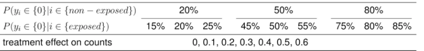
The simulation studies focus on the scenarios that structural zeros are present in the data, and there is only one binary covariate in both the structural zero part and the count component. The binary covariatexiis defined as an indicator of the exposed group and the probability of an individual coming from the exposed group is set as 50%. 1000 subjects are generated in each simulation.
(fi) =β0+β1xi. Then, ifZi= 1, we set the outcomeYito be zero; and ifZi= 0, we simulateYi from either a Poisson distribution withYi*Poisson(exp(γ0+γ1xi)) for ZIP distributed data
or a NB distribution withYi*NB(exp(γ0+γ1xi),κ) for ZINB distributed data.
We consider a factorial design in which the factors are the proportion of zero inflation in the unexposed group, the exposure effect on the count component, as well as on the structural zeros (Fig 1).
We generate 1,000 datasets for each simulation scenario and fit the data using different methods such as LOLS, Poisson, NB, ZIP, ZINB, PH, NBH, and 2P-LOLS assuming that the exposed/unexposed group indicatorXis the only predictor in the models. For the hurdle/ ZI models,Xis the predictor for both the probability of zeros/structural zeros and the count com-ponent. For comparison, we also apply the non-parametric WRS, 2P-WRS, OLS and logistic regression in the hypothesis testing in the significance of the exposure effect. The flowchart of the simulation studies is shown inFig 2.
Results
We compare the model fitting results from different perspectives. Simulations show that, in many situations, hurdle count models (PH and NBH) produce identical fitting results as their corresponding ZI models. If the results of PH is the same as ZIP, then PH/ZIP is used to pres-ent the results for both PH and ZIP. Similarly, NBH/ZINB is used to prespres-ent the results of NBH and ZINB when their results are the same.
Hypothesis testing of the covariate effect
To test the significance of covariate effect, we perform the hypothesis test onH0:γ1= 0 vs.HA:
γ16¼0 using Wald test statistics for the one part parametric models; for the hurdle/ZI models, Fig 1. The simulation scenario.γ0= 1 for all simulation scenarios. The over-dispersion parameterκis set to be 1 for all ZINB simulation scenarios.β0
reflects the log odds of zero inflation in the unexposed group, and is equal to {−1.386, 0, 1.386} for the {20%, 50%, 80%} of zero inflation in this group.β1
reflects the change in log odds of zero inflation when changing from unexposed to exposed group. The corresponding values ofβ1of {−5%, 0, +5%} changing
in the zero inflation are {−0.349, 0, 0.287}, {0.201, 0, 0.201}, and {−0.287, 0, 0.349} for 20%, 50% and 80% of the zero inflations in the unexposed group,
repsectively.
Fig 2. The flowchart for simulation studies.
likelihood ratio test statistics is used to testH0:β1= 0 (b~1¼0for hurdle models);γ1= 0 vs.HA:
not both are equal to 0. For the WRS test, the significance test for the covariate effect is just equivalent to testing whether there is a significant location shift between the exposed and unex-posed groups. For the 2P-WRS method, we use the test statisticχ2=Z2+U2[33], whereZis the test statistic of the logistic regression for thefirst part of the model andUbeing the rank-sum statistic based on the non-zero data. This test statistic follows aχ2distribution with two degrees of freedom.
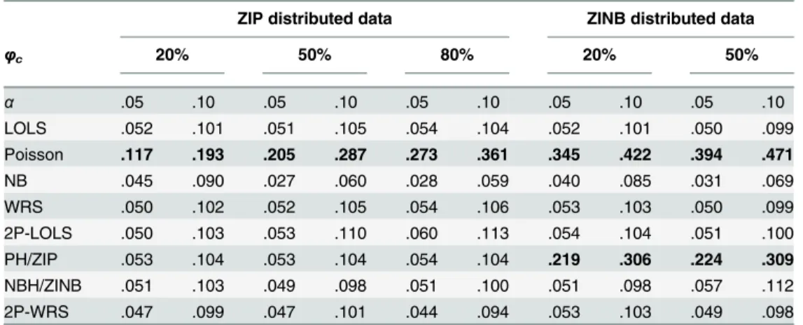
The overall type I error rates. The type I error rates are estimated using the proportion of
data sets for which the null hypothesis was falsely rejected, i.e., the percentages of detecting sig-nificant overall covariate effect for 10,000 replications when the true value ofβ1andγ1are all equal to zero.Table 1shows the estimated type I error rates at significance levelsα= {0.05,0.1} using different methods for the simulated data sets. Results show that Poisson regression has a substantially inflated type I error for both ZIP and ZINB distributed data, and so does PH/ZIP for ZINB distributed data. On the other hand, NB method yields fewer false positive than would be expected by chance, and the deflation is more obvious when the proportion of struc-tural zeros is 50% or more. The type I error rates of other methods are appropriate.
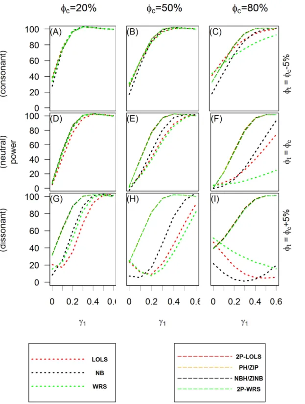
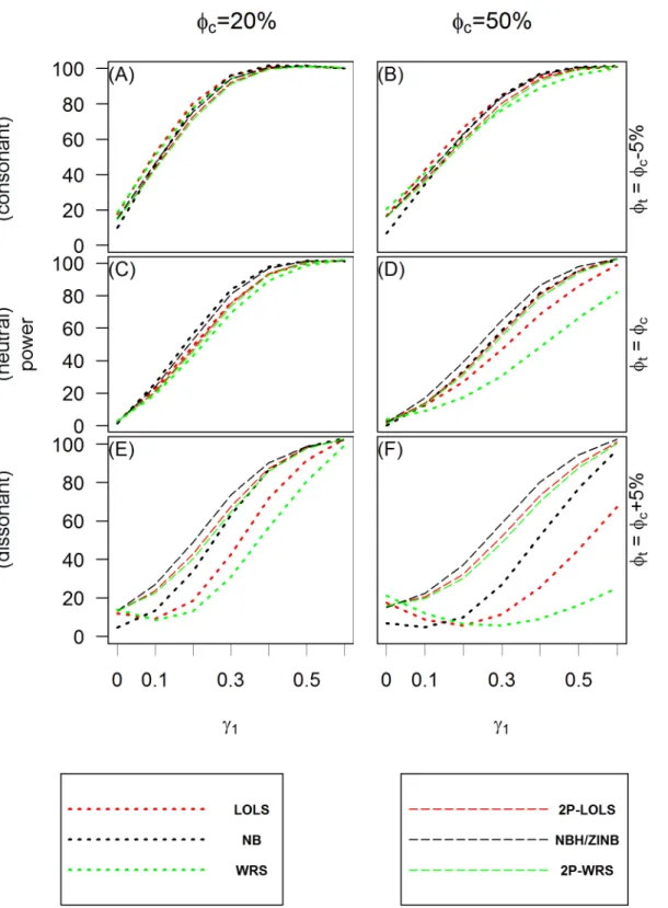
Power of test. Fig 3andFig 4show the power of test when applying different analysis
methods to the simulated ZIP and ZINB distributed data, respectively. Methods having the potential of large inflated type I errors (e.g., Poisson model or PH/ZIP model for ZINB distrib-uted data) are not included in these comparisons. These plots show that the hurdle or ZI mod-els perform consistently well in all scenarios examined, while the behaviors of one part modmod-els vary across different methods and simulation scenarios. In the consonant effect case, one part models such as LOLS and NB tend to do as well as ZI or hurdle models with WRS performing worse when the proportion of zeros is large. However, in dissonant effect cases, one part mod-els fail to have good power to detect the significance of the overall covariate effect. This is con-sistent with the observation by Lachenbruch [17] for the continuous non-negative responses with excess zeros. In the neutral effect case, when the proportion of structural zeros is 50% or more, the one-part models also have lower power than the two part models.
Table 1. The type I error rate estimations.
ZIP distributed data ZINB distributed data
φc 20% 50% 80% 20% 50%
α .05 .10 .05 .10 .05 .10 .05 .10 .05 .10
LOLS .052 .101 .051 .105 .054 .104 .052 .101 .050 .099
Poisson .117 .193 .205 .287 .273 .361 .345 .422 .394 .471
NB .045 .090 .027 .060 .028 .059 .040 .085 .031 .069
WRS .050 .102 .052 .105 .054 .106 .053 .103 .050 .099
2P-LOLS .050 .103 .053 .110 .060 .113 .054 .104 .051 .100
PH/ZIP .053 .104 .053 .104 .054 .104 .219 .306 .224 .309
NBH/ZINB .051 .103 .049 .098 .051 .100 .051 .098 .057 .112
2P-WRS .047 .099 .047 .101 .044 .094 .053 .103 .049 .098
Estimates are based on 10,000 replicated samples.φcis the probability ofycoming from structural zeros
for the unexposed group.αis the significant level of test. A bold value represents inflated type I error.
Fig 3. The power of test for ZIP simulated data.TheXaxis is the value of the covariate effect on the count dataγ1and theYaxis is the power of test when the level of significance is 0.05. Three different cases of covariate effect, i.e., the consonant (φt=φc−5%), neutral (φt=φc) and dissonant (φt=φc+ 5%)
effect, are presented in panels(A),(B)and(C);(D),(E)and(F); and(G),(H)and(I), respectively. Each column reflects different proportion of zero inflation in the unexposed group: 20% in(A),(D)and(G); 50% in(B),(E)and(H); and 80% in(C),(F)and(I)from the first to the third column.
Fig 4. The power of test for ZINB simulated data.TheXaxis is the value of the covariate effect on the count dataγ1and theYaxis is the power of test when the level of significance is 0.05. Three different cases of covariate effect, i.e., the consonant (φt=φc−5%), neutral (φt=φc) and dissonant (φt=φc
+ 5%) effect, are presented in panels(A)and(B);(C)and(D); and(E)and(F), respectively. Each column reflects different proportion of zero inflation in the unexposed group: 20% in(A),(C)and(E); and 50% in(B),(D)and(F)from the left to the right column, respectively.
Estimation of the covariate effects
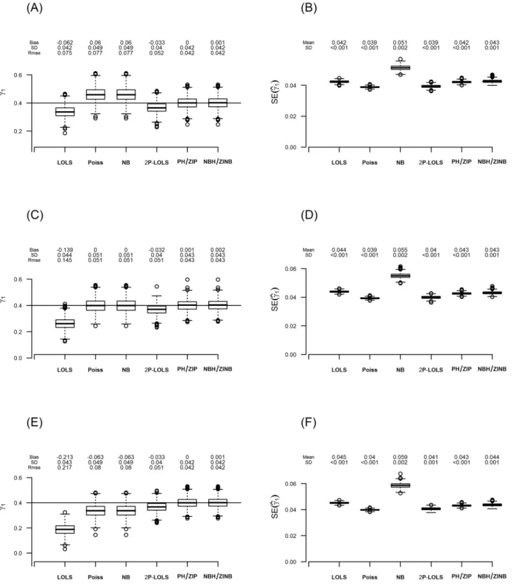
Covariate effectγ1. We first examine the covariate effect estimates and their SEs on the
log scale of count data levelsγ1.Fig 5andFig 6are the box plots of the estimation results ofγ1
and their standard errors (SEs) for ZIP and ZINB distributed data, respectively, when the true proportion of inflated zeros for unexposed group is 20%and the true value ofγ1is equal to 0.4.
Notice that for every method investigated, the standard deviation (SD) of the estimations for ZINB distributed data are larger than those for ZIP distributed data.
For both ZIP and ZINB distributed data, the pattern of estimation bias of one part models varies across different scenarios. For example, Poisson and NB have unbiased estimation in neutral effect case, but over-estimate in consonant effect and under-estimate in the dissonant effect scenario. LOLS under-estimates in all scenarios, but the absolute value of bias increases as the scenario changes from consonant to neutral, and then to dissonant effect case. The esti-mation performances of one part models for higher degree of zero inflation show similar pat-terns (S1 Fig,S2 Fig, andS3 Fig).
On the other hand, the performance of the hurdle and ZI models are consistent across dif-ferent covariate effect scenarios and difdif-ferent degrees of zero inflation. For ZIP distributed data, both PH/ZIP and ZINB/NBH give unbiased estimation ofγ1. For ZINB distributed data,
only NBH/ZINB give unbiased estimation, while PH/ZIP show under-estimation. 2P-LOLS shows improvement than LOLS, but still under-estimates the parameter especially for ZINB distributed data.
We also compare the SE estimation with the sample SD of the estimations. The estimation for SE is significantly deflated for the Poisson method. Deflation in SE can also be seen in PH/ ZIP method for ZINB distributed data. On the other hand, NB over-estimates SE, although to a lesser degree. For the ZIP distributed data with 80% zero inflation, NB has some outliers in the estimation of SE, showing unstableness of this method for a high-degree of zero inflation. The SE estimations for other methods are similar to the sample SDs of the estimates. The conse-quence of the incorrect SE estimation is wrong calculation of p-value and the misleading con-clusion about the significance effect test. For example, under-estimated SE can result in enlarged Z value and consequently smaller p-value. On the other hand, over-estimation of SE can yield incorrectly larger p-value.
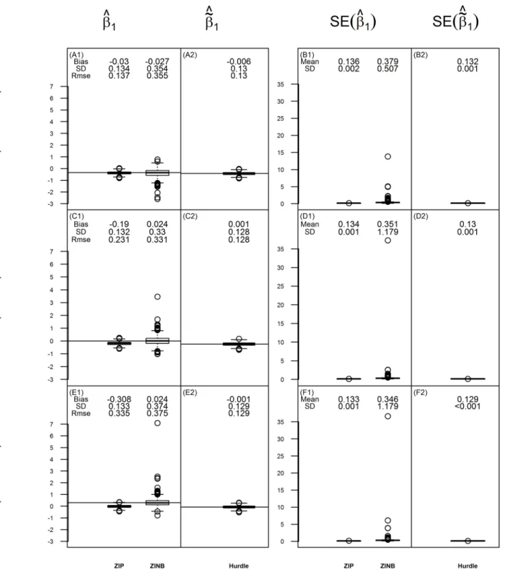
Covariate effect on the probability of (structural) zeros. Fig 7shows the boxplots of
esti-mations and their SEs forβ1using ZI models and forb~1using hurdle models when ZINB simu-lated data has 20% zero inflation in the unexposed group andγ1= 0.4. The true values of~b1are derived from the parameter estimations of the ZI model using Equation1and2. Results for other simulation settings are shown inS4 Fig,S5 Fig,S6 Fig,S7 Fig. Because the logistic regres-sion part is the same, the estimations forb~1are identical across different hurdle models. Simi-larly to the case ofγ1, ZINB has unbiased estimation ofβ1for both ZIP and ZINB distributed data, while ZIP is only unbiased for ZIP distributed data. Notice that when the proportion of zero inflation is low (e.g.,fc= 20%), ZINB may have unstable results with some large SE. The estimations are more stable when the zero inflation proportion increases to 50% or when the sample size is increased (results not given). On the contrary, hurdle models give unbiased and stable estimates for~b1in all simulation scenarios.
AIC values
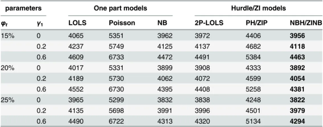
Table 2shows the mean of the AICs from simulations under ZINB distribution whenfc=
Fig 5. The estimate ofγ1and its standard error for data simulated under ZIP withϕc=20%. The figure displays box-plots of estimates and their standard errors forγ1from 1000 replications in(A)and(B);(C)and(D); and(E)and(F)for the consonant (φt=φc−5%), neutral (φt=φc) and dissonant (φt=
φc+ 5%) effect case, respectively. For each box of the boxplots, the center line represents the median, the bottom line represents the 25th percentiles and
the top line represents the 75th percentiles. The whiskers of the boxplots show 1.5 interquartile range (IQR) below the 25th percentiles and 1.5 IQR above the 75th percentiles, and outliers are represented by small circles. The horizontal line in(A),(C)and(E)represents the true value ofγ1(= 0.4) and the bias,
standard deviation (SD), and root mean square error (RMSE) of the estimations ofγ1are shown above its box-plot for each method. The mean and standard
with the smallest AIC values for each simulation scenario. For ZIP distributed data, the AICs of NBH/ZINB are very close to those of PH/ZIP. However, for ZINB distributed data, PH/ZIP has much larger AICs than the true model. Except in the case of fitting PH/ZIP to ZINB dis-tributed data, hurdle/ZI models in general have smaller AICs than one-part models. Among all the one-part models, NB has the smallest AIC values and for ZINB distributed data with rela-tively small proportion (e.g., 20%) of excess zeros, it shows better performance than 2P-LOLS.
Evaluation of model selection procedure
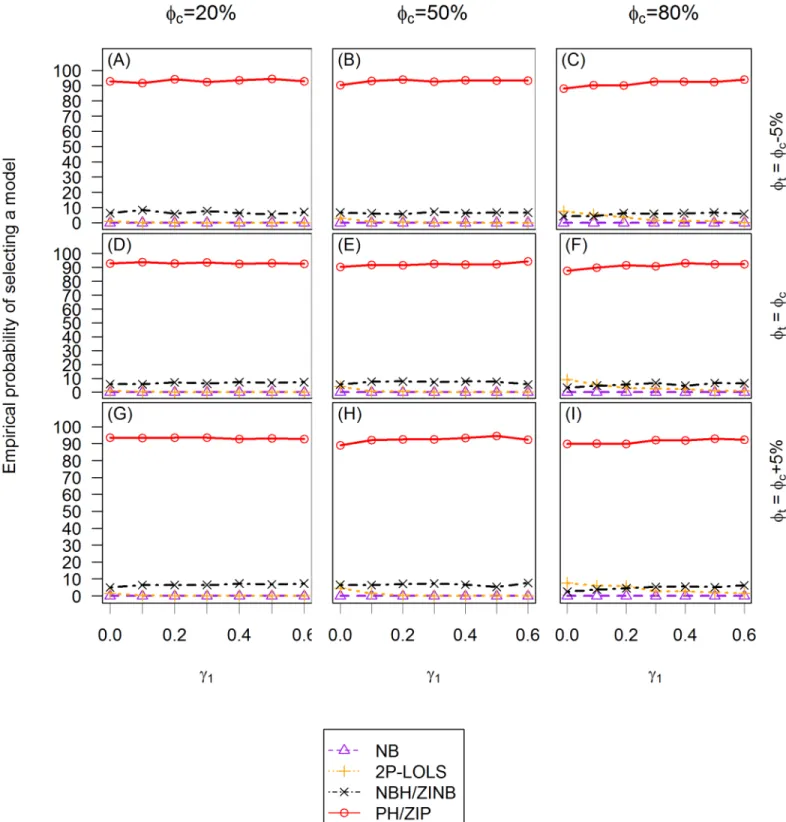
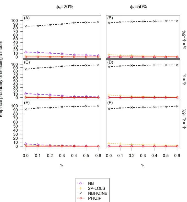
We examine the ability to select the correct model based on AICs. We also evaluate the perfor-mance of Vuong test in the testing of ZINB vs. NB model for the ZINB distributed data. We illustrate the empirical probability of selecting different models using AIC criterion inFig 8 andFig 9. Notice that in these simulation studies, because of the binary covariate setting, a ZI model and its corresponding hurdle model have identical AIC values. However, AIC values can be different if continuous covariates are involved [27].
The AIC criterion never selects LOLS nor Poisson models in either ZIP or ZINB distributed data, therefore only NB, 2P-LOLS, PH/ZIP, and NBH/ZINB models are compared. For ZIP distributed data, the plots show that the empirical probabilities of identifying the correct model (i.e., PH/ZIP) are similar across different simulation settings and are around 90%. At about 3–10% of the time, the AIC criterion favors NBH/ZINB model. Whenγ1is small (e.g.,<0.2) and the degree of zero inflation is relatively large, 2P-LOLS is chosen at about 3–15% of the time as the best model. However, ifγ1is sufficiently large, the chance of choosing the 2P-LOLS becomes rare. The AIC criterion never identifies the ZIP distributed data as NB distributed. For ZINB distributed data, 85- 99% of the time, the AIC model selection procedure will identify the correct distribution (i.e., NBH/ZINB). The probability of the correct identification has smallest value atγ1= 0 whenfc= 20%, but increases with the increasing ofγ1value and the
zero inflation degree. Whenfc= 20%, the AIC performance has some slight discrepancies among different covariate effect scenarios, with the dissonant effect case having the largest, and the consonant effect case having the smallest correct model identification percentage. The most common mis-specified model for the ZINB distributed data is NB (3–15% of the time) whenfc= 20%, and 2P-LOLS (1–7% of the time) whenfc= 50%. PH/ZIP is never identified as the best model for ZINB distributed data.
Examination of the Vuong test of ZINB vs. NB for the ZINB distributed data whenfc= 20% shows that Vuong test has lower power than AIC criterion in the selection of correct model (results not given in plots or tables). The result shows that about 60% of the time, the Vuong test favors ZINB over NB whenγ1= 0. Similar to the AIC criterion, the percentage of the correct model identification increases with the increasing ofγ1value. Whenfc= 50%, more than 96% of the time the Vuong test will select the correct model.
Fig 6. The estimate ofγ1and its standard error for data simulated under ZINB withϕc= 20%.The figure displays box-plots of estimates and their standard errors forγ1from 1000 replications in(A)and(B);(C)and(D); and(E)and(F)for the consonant (φt=φc−5%), neutral (φt=φc) and dissonant (φt=
φc+ 5%) effect case, respectively. For each box of the boxplots, the center line represents the median, the bottom line represents the 25th percentiles and
the top line represents the 75th percentiles. The whiskers of the boxplots show 1.5 interquartile range (IQR) below the 25th percentiles and 1.5 IQR above the 75th percentiles, and outliers are represented by small circles. The horizontal line in(A),(C)and(E)represents the true value ofγ1(= 0.4) and the bias, standard deviation (SD), and root mean square error (RMSE) of the estimations ofγ1are shown above its box-plot for each method. The mean and standard deviation (SD) of the standard error (SE) estimations are shown above the box-plot for each method in panels(B),(D)and(F).
Fig 7. The estimate ofβ1(or~b1) and its standard error for data simulated under ZINB whenφc=20%andγ1=0.4. Thefigure displays box-plots of estimates and their standard errors for the covariate effect on the log-odds of structural zeros for ZIP and ZINB method and on the log-odds of zeros for hurdle models from 1000 replications whenγ1= 0.4. For each box of the boxplots, the center line represents the median, the bottom line represents the 25th percentiles and the top line represents the 75th percentiles. The whiskers of the boxplots show 1.5 interquartile range (IQR) below the 25th percentiles and 1.5 IQR above the 75th percentiles, and outliers are represented by small circles. Panels(A1),(C1)and(E1)show the estimates ofβ1for consonant, neutral
Application to human microbiome study
The specific objective of the Genetic Environmental Microbial (GEM) project is to define the risk factors that lead to the onset of Crohn0s disease through the study of individuals before they develop the disease. Healthy first degree relatives of people with Crohn0s disease, predomi-nantly siblings and offspring, are recruited. Each subject provides a stool sample and bacterial DNA is extracted. The V4 hypervariable region of bacterial 16S rRNA gene are sequenced in paired-end modules (2 × 150 bp) on Illumina MiSeq platform. The resulting paired reads are assembled using paired-end assembler for Illumina sequences PANDAseq v2.7 [35] to generate an amplicon size of 253 base pairs. Assembled reads are demultiplexed and analyzed using Quantitative Insights into Microbial Ecology (QIIME) software v1.8 [36]. For quality filtering, the default parameters of QIIME are maintained. Chimeric sequences are identified and removed using usearch61 [37]. To identify OTUs from the non-chimeric sequences we use a closed reference-based picking approach using UCLUST software against Greengenes database 13_8 of bacterial 16S rRNA sequences. The abundance of a specific bacterial genus can be obtained by aggregating all the counts of assigned sequences to this genus.
In this paper, we choose three organisms to represent the range of overall percentage of zeros, in which Anaerotruncus has a small proportion of zero counts (18%), Dehalobacterium is intermediate (50%) and Campylobacter is high (77%). Histograms for the abundance of these bacteria (S8 Fig) all exhibit right skewed and over-dispersion. There are 204 males and 262 females, and it is of interest to determine whether there is a significant sex difference in the abundance of each of these bacteria. A two sample t-test shows that the mean age of males (19.2 years) is significantly younger than that of females (21.2 years,p= 0.006). Therefore, age (E1). Panels(A2),(C2)and(E2)show the estimates ofb~1for consonant, neutral and dissonant effect case, respectively. The horizontal line in these panels represents the true value of~b1, which is−0.420 in(A2),−0.240 in(C2)and−0.070 in(E2). The bias, standard deviation (SD), and root mean square error
(RMSE) of the estimates are shown above the box-plot for each method. Panel(B1),(D1)and(F1)show the SEs of the estimates forβ1, and panel(B2),(D2)
and(F2)show the SEs of the estimates for~b1. The mean and standard deviation (SD) of the standard error (SE) estimations are shown above the box-plot for each method.
doi:10.1371/journal.pone.0129606.g007
Table 2. The AIC’s of different methods for data simulated under ZINB distribution withϕc= 20%.
parameters One part models Hurdle/ZI models
φt γ1 LOLS Poisson NB 2P-LOLS PH/ZIP NBH/ZINB
15% 0 4065 5351 3962 3972 4406 3956
0.2 4237 5749 4125 4137 4682 4118
0.6 4609 6733 4472 4491 5384 4463
20% 0 4017 5331 3899 3908 4333 3892
0.2 4189 5730 4062 4072 4599 4054
0.6 4552 6730 4395 4408 5258 4381
25% 0 3965 5299 3832 3838 4248 3822
0.2 4135 5698 3991 3996 4501 3979
0.6 4490 6722 4313 4320 5134 4294
The numbers are the mean of the AIC’s for 1000 replications.φcis the probability ofycoming from
structural zeros for the unexposed group.φtis the probability ofycoming from structural zeros for the
exposed group. The smallest AIC values among allfitting models are displayed in bold font.
Fig 8. The empirical probability of choosing a model using AIC criterion for ZIP distributed data.TheXaxis is the value of the covariate effect on the count dataγ1and theYaxis is the empirical probability of choosing a model using AIC criterion. Three different cases of covariate effect, i.e., the consonant
(φt=φc−5%), neutral (φt=φc) and dissonant (φt=φc+ 5%) effect, are presented in(A),(B)and(C);(D),(E)and(F); and(G),(H)and(I), respectively. Each
column reflects different proportion of zero inflation in the unexposed group: 20% in(A),(D)and(G); 50% in(B),(E)and(H); and 80% in(C),(F)and(I)from the first to the third column.
Fig 9. The empirical probability of choosing a model using AIC criterion for ZINB distributed data.TheXaxis is the value of the covariate effect on the count dataγ1and theYaxis is the empirical probability of choosing a model using AIC criterion. Three different cases of covariate effect, i.e., the consonant
(φt=φc−5%), neutral (φt=φc) and dissonant (φt=φc+ 5%) effect, are presented in(A)and(B);(C)and(D); and(E)and(F), respectively. Each column
reflects different proportion of zero inflation in the unexposed group: 20% in(A),(C)and(E); and 50% in(B),(D)and(F)from the left to the right column, respectively.
is included as an additional covariate in the model to adjust for possible confounding. The total number of reads varies among subjects with a mean of 71,490. (SD = 32,839,S9 Fig.).
We fit the data using the different models discussed, including both gender and age as covariates. For the hurdle/ZI models, they are also covariates for the zero component. We choose female as the reference category for gender. Considering the variation in the total num-ber of sequence counts across samples, we use the log-transformed total numnum-ber of reads as an offset in a log linear regression model for LOLS, Poisson, NB models, and for the count compo-nent of the hurdle/ZI models such as 2P-LOLS, PH, NBH, ZIP and ZINB. We also use it as an offset for the logistic regression part of hurdle models. Results are shown inTable 3for Cam-pylobacter, and inS5 TableandS6 TableTables for Anaerotruncus and Dehalobacterium. The flowchart of the data analysis is shown inFig 10.
For Campylobacter with 77% zeros (Table 3), NB, NBH and ZINB has the first, second and third smallest AICs, respectively, and the AIC values are very close. In addition, all of these models consistently detect a significant gender effect, while other models do not. Furthermore, their predictions (Fig 11) are similar and can describe the observed sequence counts very well. They also perform about the same in the estimations ofγ1. However, the ZINB provides a
rela-tively large SE forb^1, indicating the lack of stability of the parameter estimate in the ZINB parameterization. Vuong test shows no particular preference for any of these three models. We thus choose NB as thefitting model and conclude that gender is significantly associated with the OTU count levels of Campylobacter, with males having significantly lower mean counts than females.
For bacteria Anaerotruncus, with 18% of zeros, all models consistently suggest significant association of its abundance with gender, but not age (Poisson family models excluded). Among all the fitted models, NBH, LOLS and NB has the first, second and third smallest AIC values, respectively. Vuong test favors NBH over NB and ZINB (p<= 0.05), but no preference Table 3. The parameter estimate of the gender effect and goodness of fit for bacteria Campylobacter (proportion of zeros: 77%) using different methods.Female is the reference category for gender.
Model Logit* Count distribution overall AIC
β1(SE) Pr(>jtj) γ1(SE) Pr(>jtj) p-value**
LOLS NA NA −0.074 (0.074) 0.316 0.316 1388
Poisson NA NA −0.782 (0.091) <10−6 <10−6 2781
NB NA NA −0.841 (0.306) 0.006 0.006 976
†
WRS NA NA NA NA 0.420 NA
2P-LOLS 0.335(0.236) 0.156 0.002 (0.220) 0.992 0.365 1051
PH 0.320(0.236) 0.174 −0.598 (0.096) <10−6 <10−6 1792
ZIP 0.226(0.237) 0.342 −0.599 (0.096) <10−6 <10−6 1793
NBH 0.320(0.236) 0.174 −0.923 (0.470) 0.049 0.059 978
††
ZINB 0.022(3.567) 0.995 −0.813 (0.410) 0.047 0.047 981†††
2P-WRS NA NA NA NA 0.597 NA
The standard errors (SEs) of estimations are in parentheses. Thefirst, second and third smallest AIC value among different models (except logistic regression) are displayed with superscript†
,††
, and†††
respectively. The model with its name in bold font is thefinal selected model.
*:logitðfiÞ ¼logð
fi
1fiÞ ¼X
T
ib, whereφis the probability of zeros/structural zeros as defined in hurdle/ZI models.
**: The overall p-value is the same as the p-value for the one part model. For the hurdle/ZI models, p-value is computed uisng the likelihood ratio test statistics in testingH0:β1= 0,γ1= 0 vs.HA: not both are equal to 0.
Fig 10. The flowchart for microbiome real data analysis.
between NB and ZINB.Fig 11shows that these three models perform similarly on the predic-tion of the counts of 2 or more. However, NB appears to overestimate the probability of zero counts for females but underestimates it for males. LOLS underestimates zero counts for both females and males. For NBH, the predicted probability of zero counts matches the observed probability. Notice that ZINB has a large SE (= 24.705) for^b1suggesting non-convergence of the ZINB model. Therefore we choose NBH as the most appropriate model and conclude that there is a significant association between gender and the abundance of bacteria Anaerotruncus. This association is through the effect of gender on the probability of zero OTU counts, with males having higher chance of having zero counts.
For Dehalobacterium, with 50% of zeros, NBH, ZINB and NB has the first, second and third smallest AICs, respectively. Vuong test has the same order of model favor (p<0.01). We thus choose NBH as the most appropriate model for the OTU counts of this bacteria. Note that the predictions from ZINB and NBH model are indistinguishable and they describe the data better than NB model (Fig 11). An inspection of the fitting results using formulapðy2 f0gÞ ¼
expðb0þb1Sexþb2AgeÞ
1þexpðb0þb1Sexþb2AgeÞshows that the proportion of structural zeros identified by a ZINB model is
about 40%. If we are interested in modeling these structural zeros, then the ZINB model should be used instead. Notice that all models suggest insignificant gender effect on the sequence counts, and we thus conclude that there is no significant association between gender and the abundance of Dehalobacterium.
Discussion
In microbiome research, count data with excess zeros is commonly encountered. To assess the importance of accounting for zero inflation and the consequence of mis-specifying the statisti-cal models, we designed a comprehensive simulation study and compared the performance of different competing methods under a variety of scenarios such as different degrees of zero inflation, different directions of covariate effect on the structural zero and count components, and variation of the count component from equi- to over-dispersion. We focused on the assess-ment of type I error, power to detect overall covariate effect, measures of model fit, and bias and effectiveness of parameter estimations.
Results confirm that if the data is zero inflated, standard one part models in general will fail to provide a good model fit, which may result in biased and inefficient parameter estimations and the possibility of type I error or loss of power. Particularly, Poisson regression has substan-tially inflated type I errors and thus is not suitable for count data with excess zeros. On the con-trary, NB has less type I errors than expected and may be prone to reduced power. Although LOLS has well-controlled type I error rates and competitive power in the consonant case, it is not robust to other situations of covariate effects. Furthermore, one part models tend to under-estimate the frequencyies of zeros and have biased estimation of the covariate effect size, which may result in incorrect sample size estimation needed for replication studies.
The ZIP and ZINB models were specifically developed for count data with structural zeros. Among the two ZI models, ZINB is more robust since it can handle both over- and equi-dis-persion in the count component, while ZIP is only suitable for the later scenario. The ZI regres-sions allow us to investigate not only the possible association of environmental or genetic factors with the count levels, but also their associations with the probability of structural zeros.
more stable parameter estimations for both the zero and count components and they are robust if there is no zero inflation and can handle zero deflation problems [25]. Furthermore, the fit-ting indices (such as AICs) and the estimation of the effect for the magnitude of the count data from the corresponding hurdle and ZI models are similar. Therefore, due to the computational consideration, if the interest is in prediction or if the data-generating mechanism of the zeros is unknown, we suggest to choose PH or NBH (depending whether over-dispersion is present in the count component) over the ZI models. However, if the study goal is in statistical inference, the model choice should also be adjusted by clinical reasoning [23]. If structural zeros are believed to exist and the interest is in modeling them, the ZI models should be chosen. In this case, if non-convergence is encounter, then a larger sample size is probably required.
Other hurdle models such as 2P-LOLS and 2P-WRS show relatively comparable power to the true ZIP or ZINB model and have well-controlled type I errors in testing the overall covari-ate effect. Furthermore, they are robust for the case of over-dispersion in the count component and thus can be considered if we are just interested in the testing of association. However, due to its mis-specification of the counts as the continuous normally distributed data, 2P-LOLS will in general result in biased parameter estimation of the covariate effects and is thus not recom-mended for statistical inference on the bacterial counts. 2P-WRS cannot be used for statistical inference either.
As this simulation study has shown, the inappropriate application of a statistical model could have undesirable consequences. Therefore, it is important for researchers to perform model selection to choose the most appropriate model. Our simulation confirms that the AIC criterion has good power in identifying the correct distribution of the data and Vuong test has less power. However, caution should be given for the possibility of model mis-identification using these selection strategies. For example, for the ZINB distributed data with relatively low degree of zero inflation, it is possible that NB is mis-identified as the best model. Therefore, a graphical examination of the comparison of the observed with the predicted values is recommended.
In this paper, we focus on the discussion of the simulation results for binary covariate case. Additional simulations are also conducted (results not given) for a continuous covariate and we have similar observations as in the case of a binary covariate. Particularly, although not exactly identical, the AIC value produced by NBH and ZINB model are very close and are the smallest among all fitted models. We also evaluate the overall type I error and power of test for two other commonly used models: OLS and logistic regression (Results are provided inS7 Table,S10 FigandS11 Fig). Both OLS and logistic regression have well-controlled type I error rates. It is interesting to see that OLS performs well in terms of power in the consonant effect scenario. However, similar to other one-part models, it is not robust to other scenarios (i.e., dis-sonant or neutral effects). The supplementary material also provides the evaluation results of relative bias of prediction for zeros for the competing models (S8 Table,S9 Table,S10 Table, S11 TableandS12 Table). All the one part models underestimate the probability of the zeros while the hurdle and ZI count models (i.e., PH, ZIP, NBH, ZINB) show unbiased estimations. 2P-LOLS has small bias, and the bias decreases when the proportion of inflated zeros becomes higher.
counts, the red line connects the expected counts produced by the model with smallest AIC values, the green line connects the expected counts produced by the model with the second smallest AIC values and the blue line connects the expected counts produced by the model with the third smallest AIC values. The first, second and third row of the plots are for bacteria Campylobacter, Anaerotruncus, and Dehalobacterium, respectively.
Our simulation study just focuses on the independent data assumption, however, in clinical studies and the microbiome field, observations maybe serial or related say due to families, thus in future work we will extend our evaluation to the related data with excess zeros.
Supporting Information
S1 Table. The AIC’s of different methods for data simulated under ZIP distribution with
fc= 20%.The numbers are the mean of the AIC’s for 1000 replications.fcis the probability of
ycoming from structural zeros for the non-exposed group.ftis the probability ofycoming from structural zeros for the exposed group. The smallest AIC values among all fitting models are displayed in bold font.
(PDF)
S2 Table. The AIC’s of different methods for data simulated under ZIP distribution with
fc= 50%.The numbers are the mean of the AIC’s for 1000 replications.fcis the probability of
ycoming from structural zeros for the non-exposed group.ftis the probability ofycoming from structural zeros for the exposed group. The smallest AIC values among all fitting models are displayed in bold font.
(PDF)
S3 Table. The AIC’s of different methods for data simulated under ZIP distribution with
fc= 80%.The numbers are the mean of the AIC’s for 1000 replications.fcis the probability of
ycoming from structural zeros for the non-exposed group.ftis the probability ofycoming from structural zeros for the exposed group. The smallest AIC values among all fitting models are displayed in bold font.
(PDF)
S4 Table. The AIC’s of different methods for data simulated under ZINB distribution with
fc= 50%.The numbers are the mean of the AIC’s for 1000 replications.fcis the probability of
ycoming from structural zeros for the non-exposed group.ftis the probability ofycoming from structural zeros for the exposed group. The smallest AIC values among all fitting models are displayed in bold font.
(PDF)
S5 Table. The parameter estimate of the gender effect and goodness of fit for bacteria
Anae-rotruncus (proportion of zeros: 18%) using different methods.Female is the reference
cate-gory for gender. The standard errors (SEs) of estimations are in parentheses. The first, second and third smallest AIC value among different models (except logistic regression) are displayed with superscript†,††, and†††respectively. The model with its name in bold font is the final selected model.:logitðf
iÞ ¼logð fi
1 fiÞ ¼X T
ib, wherefis the probability of zeros/structural
zeros as defined in hurdle/ZI models.: The overall p-value is the same as the p-value for the
one part model. For the hurdle/ZI models, p-value is computed uisng the likelihood ratio test statistics in testingH0:β1= 0,γ1= 0 vs.HA: not both are equal to 0.
(PDF)
S6 Table. The parameter estimate of the gender effect and goodness of fit for bacteria
Deha-lobacterium (proportion of zeros: 50%) using different methods.Female is the reference
cat-egory for gender. The standard errors (SEs) of estimations are in parentheses. The first, second and third smallest AIC value among different models (except logistic regression) are displayed with superscript†,††, and†††respectively. The model with its name in bold font is the final selected model.:logitðfiÞ ¼logð
fi
1 fÞ ¼X T
zeros as defined in hurdle/ZI models.: The overall p-value is the same as the p-value for the
one part model. For the hurdle/ZI models, p-value is computed uisng the likelihood ratio test statistics in testingH0:β1= 0,γ1= 0 vs.HA: not both are equal to 0.
(PDF)
S7 Table. The type I error rate estimations for different competing models (including OLS
and Logistic regression).Estimates are based on 10,000 replicated samples.fcis the
probabil-ity ofycoming from structural zeros for the non-exposed group.αis the significant level of test. A bold value represents inflated type I error.
(PDF)
S8 Table. The relative bias for P(y = 0) for data simulated under ZIP distribution withfc=
20%.The numbers are the mean of the relative bias of p(y = 0) for 1000 replications.fcis the probability ofycoming from structural zeros for the non-exposed group.ftis the probability ofycoming from structural zeros for the exposed group.
(PDF)
S9 Table. The relative bias for P(y = 0) for data simulated under ZIP distribution withfc=
50%.The numbers are the mean of the relative bias of p(y = 0) for 1000 replications.fcis the probability ofycoming from structural zeros for the non-exposed group.ftis the probability ofycoming from structural zeros for the exposed group.
(PDF)
S10 Table. The relative bias for P(y = 0) for data simulated under ZIP distribution withfc
= 80%.The numbers are the mean of the relative bias of p(y = 0) for 1000 replications.fcis the
probability ofycoming from structural zeros for the non-exposed group.ftis the probability ofycoming from structural zeros for the exposed group.
(PDF)
S11 Table. The relative bias for P(y = 0) for data simulated under ZINB distribution with
fc= 20%.The numbers are the mean of the relative bias of p(y = 0) for 1000 replications.fcis
the probability ofycoming from structural zeros for the non-exposed group.ftis the probabil-ity ofycoming from structural zeros for the exposed group.
(PDF)
S12 Table. The relative bias for P(y = 0) for data simulated under ZINB distribution with
fc= 50%.The numbers are the mean of the relative bias of p(y = 0) for 1000 replications.fcis
the probability ofycoming from structural zeros for the non-exposed group.ftis the probabil-ity ofycoming from structural zeros for the exposed group.
(PDF)
S1 Fig. The estimate ofγ1and its standard error for data simulated under ZIP distribution
withfc= 50%.The box-plot ofγ1estimates (in the left column panel) and their corresponding
SE estimates (in the right column panel) for 1000 replications of simulated ZIP data using LOLS, Poisson, NB, 2P-LOLS and ZINB methods. The horizontal line in the left column plots is the true value ofγ1, which is 0.4. The consonant, neutral and dissonant scenarios are
dis-played in the first, second and third rows, respectively. The bias, root mean square error (rmse) and standard deviation (sd) of the estimations ofγ1are shown above its box-plot for each
method in the left column. The mean and standard deviation (sd) of the standard error (SE) estimations above the box-plot for each method in the right column.
S2 Fig. The estimate ofγ1and its standard error for data simulated under ZIP distribution
withfc= 80%.The box-plot ofγ1estimates (in the left column panel) and their corresponding
SE estimates (in the right column panel) for 1000 replications of simulated ZIP data using LOLS, Poisson, NB, 2P-LOLS and ZINB methods. The horizontal line in the left column plots is the true value ofγ1, which is 0.4. The consonant, neutral and dissonant scenarios are
dis-played in the first, second and third rows, respectively. The bias, root mean square error (rmse) and standard deviation (sd) of the estimations ofγ1are shown above its box-plot for each
method in the left column. The mean and standard deviation (sd) of the standard error (SE) estimations above the box-plot for each method in the right column.
(PDF)
S3 Fig. The estimate ofγ1and its standard error for data simulated under ZINB
distribu-tion withfc= 50%.The box-plot ofγ1estimates (in the left column panel) and their
corre-sponding SE estimates (in the right column panel) for 1000 replications of simulated ZINB data using LOLS, Poisson, NB, 2P-LOLS and ZINB methods. The horizontal line in the left col-umn plots is the true value ofγ1, which is 0.4. The consonant, neutral and dissonant scenarios
are displayed in the first, second and third rows, respectively. The bias, root mean square error (rmse) and standard deviation (sd) of the estimations ofγ1are shown above its box-plot for
each method in the left column. The mean and standard deviation (sd) of the standard error (SE) estimations above the box-plot for each method in the right column.
(PDF)
S4 Fig. The estimate ofβ1(or~β1) and its standard error for data simulated under ZIP
dis-tribution withfc= 20%.Thefigure displays box-plots of estimates and their standard errors
for the covariate effect on the log-odds of structural zeroes for ZIP and ZINB method and on the log-odds of zeroes for hurdle models from 1000 replications. Panels(A1),(C1), and(E1)
show the estimates ofβ1for consonant, neutral and dissonant effect case, respectively. The hor-izontal line in these panels represents the true value ofβ1, which is−0.349 in(A1), 0 in(C1)
and 0.287 in(E1). Panels(A2),(C2), and(E2)show the estimates of~b1for consonant, neutral and dissonant effect case, respectively. The horizontal line in these panels represents the true value of~b1, which is−0.540 in(A2),−0.218 in(C2)and 0.053 in(E2). The bias, root mean
square error (RMSE) and standard deviation (SD) of the estimates are shown above the box-plot for each method. Panel(B1),(D1), and(F1)show the SEs of the estimates forβ1, and
panel(B2),(D2), and(F2)show the SEs of the estimates for~b1. The mean and standard devia-tion (SD) of the standard error (SE) estimadevia-tions are shown above the box-plot for each method.
(TIFF)
S5 Fig. The estimate ofβ1(or~β1) and its standard error for data simulated under ZIP
dis-tribution withfc= 50%.Thefigure displays box-plots of estimates and their standard errors
for the covariate effect on the log-odds of structural zeroes for ZIP and ZINB method and on the log-odds of zeroes for hurdle models from 1000 replications. Panels(A1),(C1), and(E1)
show the estimates ofβ1for consonant, neutral and dissonant effect case, respectively. The hor-izontal line in these panels represents the true value ofβ1, which is−0.201 in(A1), 0 in(C1)
and 0.201 in(E1). Panels(A2),(C2), and(E2)show the estimates of~b1for consonant, neutral and dissonant effect case, respectively. The horizontal line in these panels represents the true
value of~b1, which is−0.295 in(A2),−0.098 in(C2)and 0.100 in(E2). The bias, standard
for each method. Panel(B1),(D1), and(F1)show the SEs of the estimates forβ1, and panel
(B2),(D2), and(F2)show the SEs of the estimates for~b1. The mean and standard deviation (SD) of the standard error (SE) estimations are shown above the box-plot for each method. (TIFF)
S6 Fig. The estimate ofβ1(or~β1) and its standard error for data simulated under ZIP
dis-tribution withfc= 80%.Thefigure displays box-plots of estimates and their standard errors
for the covariate effect on the log-odds of structural zeroes for ZIP and ZINB method and on the log-odds of zeroes for hurdle models from 1000 replications. Panels(A1),(C1), and(E1)
show the estimates ofβ1for consonant, neutral and dissonant effect case, respectively. The
hor-izontal line in these panels represents the true value ofβ1, which is−0.287 in(A1), 0 in(C1)
and 0.349 in(E1). Panels(A2),(C2), and(E2)show the estimates of~b1for consonant, neutral and dissonant effect case, respectively. The horizontal line in these panels represents the true value of~b1, which is−0.349 in(A2),−0.063 in(C2)and 0.285 in(E2). The bias, standard
devi-ation (SD), and root mean square error (RMSE) of the estimates are shown above the box-plot for each method. Panel(B1),(D1), and(F1)show the SEs of the estimates forβ1, and panel
(B2),(D2), and(F2)show the SEs of the estimates for~b1. The mean and standard deviation (SD) of the standard error (SE) estimations are shown above the box-plot for each method. (TIFF)
S7 Fig. The estimate ofβ1(or~β1) and its standard error for data simulated under ZINB
dis-tribution withfc= 50%.Thefigure displays box-plots of estimates and their standard errors
for the covariate effect on the log-odds of structural zeroes for ZIP and ZINB method and on the log-odds of zeroes for hurdle models from 1000 replications. Panels(A1),(C1), and(E1)
show the estimates ofβ1for consonant, neutral and dissonant effect case, respectively. The
hor-izontal line in these panels represents the true value ofβ1, which is−0.201 in(A1), 0 in(C1)
and 0.201 in(E1). Panels(A2),(C2), and(E2)show the estimates of~b1for consonant, neutral and dissonant effect case, respectively. The horizontal line in these panels represents the true value of~b1, which is−0.315 in(A2),−0.151 in(C2)and 0.020 in(E2). The bias, standard
devi-ation (SD), and root mean square error (RMSE) of the estimates are shown above the box-plot for each method. Panel(B1),(D1), and(F1)show the SEs of the estimates forβ1, and panel (B2),(D2), and(F2)show the SEs of the estimates for~b1. The mean and standard deviation (SD) of the standard error (SE) estimations are shown above the box-plot for each method. (TIFF)
S8 Fig. The histogram of of the abundance for bacteria Anaerotruncus, Dehalobacterium
and Campylobacter.The X-axis is the possible counts of the bacterium in the square root
scale. The Y-axis is the frequency of the counts with some line breaks. (PDF)
S9 Fig. The histogram of total number of sequence counts for the bacteria classified at
genus level.The red dashed line represent the mean of the total counts (71,490) and the blue
dotted line represent the median of the total counts (65,438). The range is from 13,647 to 196,591. The standard deviation of the total counts is 32,839.
(PDF)
S10 Fig. The power of test for ZIP simulated data for competing models (including OLS
and logistic regression).TheXaxis is the value of the covariate effect on the count dataγ1and
covariate effect, i.e., the consonant (ft=fc−5%), neutral (ft=fc) and dissonant (ft=fc + 5%) effect, are presented in {(A), (B), (C)}, {(D), (E), (F)}, and {(G), (H), (I)}, respectively. Each column reflects different proportion of zero inflation in the non-exposed group: 20% in {(A), (D), (G)}, 50% in {(B), (E), (H)} and 80% in {(C), (F), (I)} from the first to the third col-umn.
(TIFF)
S11 Fig. The power of test for ZINB simulated data for competing models (including OLS
and logistic regression).TheXaxis is the value of the covariate effect on the count dataγ1and
theYaxis is the power of test when the level of significance is 0.05. Three different cases of covariate effect, i.e., the consonant (ft=fc−5%), neutral (ft=fc) and dissonant (ft=fc + 5%) effect, are presented in {(A), (B)}, {(C), (D)}, and {(E), (F)}, respectively. Each column reflects different proportion of zero inflation in the non-exposed group: 20% in {(A), (C), (E)} and 50% in {(B), (D), (F)} from the left to the right column, respectively.
(TIFF)
Acknowledgments
All authors disclose no potential conflicts (financial, professional, or personal) that are relevant to the manuscript. Williams Turpin acknowledges a CAG/CIHR Ferring Pharmaceuticals Inc. award, Lizhen Xu is a recipient of a CIHR STAGE fellowship. The authors would like to acknowledge the GEM Project Steering Committee, Recruitment Site Directors and Global Project Office members supported by Crohn’s and Colitis Canada (CCC) and the Leona M. and Harry B. Helmsley Charitable Trust. The GEM Project Research Team is composed of i) Steering Committee: Paul Beck, Charles Bernstein, Alain Bitton, Kenneth Croitoru, Leo Diele-man, Brian Faegan, Anne Griffiths, David GuttDiele-man, Kevan Jacobson, Gil Kaplan, Karen Mad-sen, John Marshall, Paul Moayyedi, Mark Ropeleski, Ernest Seidman, Mark Silverberg, Kathy Siminovitch, Andy Stadnyk, Hilary Steinhart, Michael Surette, Dan Turner, Tom Walters, and Bruce Vallance ii) Recruitment Center Directors: Guy Aumais, Paul Beck, Charles Bernstein, Alain Bitton, Brian Bressler, Herbert Brill, Maria Cino, Jeff Critch, Lee Denson, Colette Deslandres, Leo Dieleman, Martha Dirks, Wael El-Matary, Brian Feagan, Anne Griffiths, Hans Herfarth, Peter Higgins, Hien Huynh, Jeff Hyams, Kevan Jacobson, Gilaad Kaplan, Desmond Leddin, David Mack, John Marshall, Jerry McGrath, Anthony Otley, Remo Panancionne, Sophie Plamondon, Mark Ropeleski, Fred Saibil, Ernie Seidman, Corey Siegel, Mark Silverberg, Scott Snapper, Hillary Steinhart, Dan Turner and iii) The Global Project Office: Nellie Allam, Kenneth Croitoru, Alexandra Keludjian, Ana Olteanu, Kevin Ow and Isabelle Yeadon.
Author Contributions
Conceived and designed the experiments: LX ADP WT WX. Performed the experiments: LX ADP WT WX. Analyzed the data: LX WT. Contributed reagents/materials/analysis tools: LX ADP WT WX. Wrote the paper: LX ADP WT WX.
References
1. Tringe SG, von Mering C, Kobayashi A, Salamov AA, et al. (2005) Comparative metagenomics of microbial communities. Science 308 (5721): 554–557. doi:10.1126/science.1107851PMID: 15845853
3. Bäckhed F, Ding H, Wang T, et al. (2004) The gut microbiota as an environmental factor that regulates fat storage. Proc Natl Acad Sci USA 101: 15718–15723. doi:10.1073/pnas.0407076101PMID: 15505215
4. Ley RE, Bäckhed F, Turnbaugh P, et al. (2005) Obesity alters gut microbial ecology. Proc Natl Acad Sci USA 102: 11070–11075. doi:10.1073/pnas.0504978102PMID:16033867
5. Larsen N, Vogensen FK, Van den Berg FWJ, et al. (2010) Gut Microbiota in Human Adults with Type 2 Diabetes Differs from Non-Diabetic Adults. PLoS ONE 5(2): e9085. doi:10.1371/journal.pone. 0009085PMID:20140211
6. Qin J, Li Y, Cai Z, et al. (2012) A metagenome-wide association study of gut microbiota in type 2 diabe-tes. Nature 490: 55–60. doi:10.1038/nature11450PMID:23023125
7. Charles KF, Pankaj M. (2014) Identifying Keystone Species in the Human Gut Microbiome from Meta-genomic Timeseries Using Sparse Linear Regression. PLOS One 9(7): e102451. doi:10.1371/journal. pone.0102451
8. Dickson RP, Erb-Downward JR, Prescott HC, Martinez FJ, Curtis JL, et al. (2014) Cell-associated bac-teria in the human lung microbiome. Microbiome 2:28. doi:10.1186/2049-2618-2-28PMID:25206976 9. Bálint M, Tiffin P, Hallström B, O’Hara RB, Olson MS, Fankhauser JD, et al. (2013). Host genotype
shapes the foliar fungal microbiome of balsam poplar (Populus balsamifera). PLoS One 8(1):e53987. doi:10.1371/journal.pone.0053987PMID:23326555
10. Faust K, Sathirapongsasuti JF, Izard J, Segata N, Gevers D, Raes J, et al. (2012) Microbial co-occur-rence relationships in the human microbiome. PLoS Comput Biol 8(7): e1002606. doi:10.1371/journal. pcbi.1002606PMID:22807668
11. Jespers V, Menten J, Smet H, Sabrina Poradosú S, Abdellati S, Verhelst R, et al. (2012) Quantification of bacterial species of the vaginal microbiome in different groups of women, using nucleic acid amplifi-cation tests. BMC Microbiology 12:83. doi:10.1186/1471-2180-12-83PMID:22647069
12. Hauser LJ, Feazel LM, Ir D, Fang R, Wagner BD, et al. (2014) Sinus culture poorly predicts resident microbiota. International Forum of Allergy & Rhinology. doi:10.1002/alr.21428.2014/2/10
13. Loeys T, Moerkerke B, Smet OD, et al. (2012) The analysis of inflated count data: Beyond zero-inflated Poisson regression. Br J Math Stat Psych 65: 163–180. doi:10.1111/j.2044-8317.2011.02031. x
14. Yildirim S, Yeoman CJ, Janga SC, Thomas SM, Ho M, et al. (2014) Primate vaginal microbiomes exhibit species specificity without universal Lactobacillus dominance. ISME J 8 (12):2431–2444. doi: 10.1038/ismej.2014.90
15. Pearce MM, Hilt EE, Rosenfeld AB, Zilliox MJ, Thomas-Whitea K, et al. (2014) The Female Urinary Microbiome: a Comparison of Women with and without Urgency Urinary Incontinence. mBio 5(4): e01283–14. doi:10.1128/mBio.01283-14PMID:25006228
16. Dominianni Cet al. (2014) Comparison of methods for fecal microbiome biospecimen collection. BMC Microbiology 14:103. doi:10.1186/1471-2180-14-103PMID:24758293
17. Lachenbruch P. (2001) Comparisons of two-part models with competitors. Stat Med 20: 1215–1234. 18. Welsh AH, Cunningham RB, Donnelly CF, et al. (1996) Modelling the abundance of rare species:
statis-tical models for counts with extra zeros. Ecol Model 88: 297–308. doi:10.1016/0304-3800(95)00113-1 19. Lambert D. (1992). Zero-inflated Poisson regression, with an application to defects in manufacturing.
Technometrics 34: 1–14. doi:10.2307/1269547
20. Mullahy J. (1986). Specification and testing of some modified count data models. J Econometrics 33: 341–365. doi:10.1016/0304-4076(86)90002-3
21. Sileshi G, Hailu G and Nyadzi GI. (2009). Traditional occupancy—abundance models are inadequate for zero-inflated ecological count data. Ecol Model 220: 1764–1775. doi:10.1016/j.ecolmodel.2009.03. 024
22. Hu M, Pavlicova M, and Nunes E. (2011). Zero-inflated and hurdle models of count data with extra zeros: Examples from an HIV-risk reduction intervention trial. Am J Drug Alcohol Abuse 37: 367–375. doi:10.3109/00952990.2011.597280PMID:21854279
23. Rose CE, Martin SW, Wannemuehler KA, et al. (2006) On the use of zero-inflated and hurdle models for modeling vaccine adverse event count data. J Biopharm Stat 16: 463–481. doi:10.1080/ 10543400600719384PMID:16892908
24. Xia, Y., Morrison-Beedy, D., Ma, J., Feng, C., Cross, W. and Tu, X.M. (2012). Modeling count outcomes from HIV risk reduction interventions: a comparison of competing statistical models for count
responses. AIDS Research and Treatment, Article ID 593569, 11 pages. doi:10.1155/2012/593569 25. Min Y and Agresti A. (2005) Random effect models for repeated measures of zero-inflated count data.