Estimating Brazilian Monthly GDP:
a State-Space Approach
*
João Victor Issler,
†
Hilton Hostalacio Notini
‡
Contents: 1. Introduction; 2. State-Space Model and the Kalman Filter for Interpolation; 3. Empirical Results; 4. Conclusions; Appendix. Detailed Interpolation Models.
Keywords: GDP Interpolation, State-Space Representation, Kalman Filter, Composite and Leading Indicators, Nowcasting, Forecasting.
JEL Code: C32,E32, E37.
This paper has several contributions. The first is to employ a superior interpo-lation method that enables toestimate,nowcastandforecastmonthly Brazilian GDP for 1980–2012 in an integrated way—seeBernanke, Gertler, & Watson
(1997) [Systematic monetary policy and the effects of oil price shocks(Brookings Papers in Economic Activity No.1)]. Second, along the spirit ofMariano & Mura-sawa(2003) [A new coincident index of business cycles based on monthly and quarterly series. Journal of Applied Econometrics, 18(4), 427–443], we propose and test a myriad of interpolation models and interpolation auxiliary series— all coincident with GDP from a business-cycle dating point of view. Based on these results, we finally choose the most appropriate monthly indicator for Brazilian GDP. Third, this monthly GDP estimate is compared to an economic ac-tivity indicator widely used by practitioners in Brazil—the Brazilian Economic Activity Index (IBC-Br). We found that our monthly GDP tracks economic ac-tivity better than IBC-Br. This happens by construction, since our state-space approach imposes the restriction (discipline) that our monthly estimate must add up to the quarterly observed series in any given quarter, which may not hold regarding IBC-Br. Moreover, our method has the advantage to be easily im-plemented: it only requires conditioning on two observed series for estimation, while estimating IBC-Br requires the availability of hundreds of monthly series. Third, in a nowcasting and forecasting exercise, we illustrate the advantages of our integrated approach. Finally, we compare the chronology of recessions of our monthly estimate with those done elsewhere.
Esse artigo tem três contribuições originais. A primeira é o emprego de uma técnica superior de interpolação para o PIB brasileiro em bases trimestrais para a frequência mensal, método este que auxilia no nowcast e na previsão fora da amostra do cres-cimento do PIB de forma integradaBernanke, Gertler, & Watson(1997) [Systematic
*We gratefully acknowledge the comments of participants at CIRET 2008 in Santiago, Chile. We also thank Regis Bonelli and Silvia
Matos for allowing us to reproduce the results of their nowcast exercise. All errors are ours. We thank Marcia Waleria Machado, Marcia Marcos, and Rafael Burjack for excellent research assistance and thank CNPq-Brazil, FAPERJ and INCT for financial support.
†Escola Brasileira de Economia e Finanças / Fundação Getúlio Vargas (EPGE/FGV). Praia de Botafogo 190, sala 1100, Rio de Janeiro
– RJ, Brasil. CEP 22250-900. E-mail:[email protected]
monetary policy and the effects of oil price shocks(Brookings Papers in Econo-mic Activity No.1)]. A segunda, no espírito deMariano & Murasawa(2003) [A new coincident index of business cycles based on monthly and quarterly series.Journal of Applied Econometrics, 18(4), 427–443], é a de propor e testar uma miríade de modelos de interpolação e de séries auxiliares para interpolar o PIB, sendo as últi-mas todas coincidentes ao PIB do ponto de vista dos ciclos de negócios da economia brasileira. Baseados nesses resultados, escolhemos o melhor modelo para estimar o PIB brasileiro em bases mensais. A terceira é a comparação entre as dentro e fora da amostra entre a nossa série de PIB mensal e um indicador do PIB mensal popu-larmente utilizado pelo mercado financeiro — o Índice de Atividade Econômica do Banco Central (IBC-Br). Nessas comparações, notamos que o nosso indicador do PIB mensal não só segue mais de perto as variações do PIB dentro da amostra, como também o prevê de forma mais precisa fora da amostra. O primeiro resultado é es-perado, pois impomos a disciplina de que as variações trimestrais do PIB mensal devam ser iguais às do PIB trimestral. Porém, impor essa disciplina ao PIB interpo-lado também melhora a previsão fora da amostra do modelo que o contém, algo que a técnica de interpolação em si não poderia garantir, mas que observamos na prá-tica. Esse resultado aponta na direção de que talvez a construção da série mensal do IBC-Br não seja muito eficiente, pois requer o armazenamento e acompanhamento de centenas de séries mensais, enquanto a construção do nosso PIB mensal requer apenas o armazenamento e acompanhamento de duas séries auxiliares.
1. INTRODUCTION
Any modern society is concerned with its current “state” of economic activity and what should be that state in the near future. Entrepreneurs and individuals are interested in the question because their profits and welfare are a function of it. Governments also have an interest in the subject for budgetary and welfare issues.
For the U.S., the most educated estimate of economic-activity turning points is embodied in the binary variable announced by the NBER Business Cycle Dating Committee: recession vs. expansion for any given month. These announcements are based on the consensus of a panel of experts, and they are made some time (usually six months to one year) after a turning point in the business cycle has occurred. So, today, we only possessolddating’s for the state of the economy. An alternative to infer business-cycle conditions would be to use Gross Domestic Product (GDP). Indeed,Stock & Watson(1989) argue that, if we were to choose one variable to best represent the state of the economy, this variable would be GDP. They claim that “[…] fluctuations in aggregate output are at the core of the business cycle so the cyclical component of real GDP is a useful proxy for the overall business cycle […]”.
Unfortunately, GDP is also not timely available to continuously infer what is the current state of the economy. First, as far as we know, all countries compute GDP on a quarterly and/or on an annual frequency, but not on a monthly frequency. Second, there are delays in the release of quarterly GDP. Of course, delays vary across countries. In Brazil the delay in the initial release of quarterly GDP is bigger than three months and can reach up to six months at times. Moreover, this initial release is subject to major revisions in six months’ time.
The fact that a given statistic is only available with some delay does not invalidate its later use for inference if we possess a long-span time-series of it. Indeed, referring to the decisions of the NBER Business Cycle Dating Committee,Issler & Vahid(2006) argue that:
of a blood test. However, blood samples cannot be taken too frequently, and test results are only available with a lag, sometimes too long to be useful. Our index therefore must be a function of variables such as blood pressure, pulse rate and body temperature that are readily available at regular frequencies. In order to estimate the best way to combine these variables into an index, would we (i) use the historical data on these variables only, or, (ii) use the historical blood test results as well? The answer is, obviously, the latter.
Here, GDP and NBER dating are the equivalent to the results of the blood test. What should be the equivalent to blood pressure, pulse rate and body temperature? Since the pioneering work ofBurns & Mitchell(1946), we have been endowed with coincident and leading indicators of economic activity, which are timely proxies, respectiverly, of the current state of economic activity and what will it be in the near future. This suggests that a superior strategy for having timely and more frequent estimates of eco-nomic activity is to combine GDP (or NBER dating) with information on these timely proxies. Issler and Vahid focused on combining NBER dating information with coincident and leading series of economic activity. Our focus here will be to combine the latter data for Brazil with Brazilian GDP.
As argued above, this strategy can improve our knowledge of GDP in two dimensions. The first is that we will possess more frequent business-cycle estimates, i.e., monthly instead of quarterly. This solves an interpolation problem that was proposed byBernanke, Gertler, & Watson(1997) with an econometric model that encompassed most interpolation models that had been previously proposed in the literature; see also the extension inMönch & Uhlig(2005). The second is that we will be able tonowcastandforecast
GDP using information on coincident and leading series of economic activity. This solves anowcasting
problem, to say the least, and has been proposed byMariano & Murasawa(2003).
The main contributions of this paper are twofold. First, we propose a joint model for Brazilian GDP and Brazilian coincident series that can be used to interpolate and nowcast GDP. Our model is based on the encompassing methods proposed byBernanke et al.(1997) and inMönch & Uhlig(2005). Second, for forecasting, we will propose an alternative model for Brazilian GDP and Brazilian leading series. It is essentially an extension of the model proposed byMariano & Murasawa(2003)—who are mostly concerned with nowcasting—but will be used for forecasting purposes since we will switch the roles of coincident and leading series in implementing the model. As is clear, our main contribution is empirical, although our motivation to use and combine currently available methods is somewhat original.
In the business-cycle dimension, the ideas and models discussed in this paper are also related to the work ofStock & Watson(1988,1991,1993a,1993b,2002a,2002b),Chauvet(1998),Kim & Nelson(1999),
Cuche & Hess(2000),Liu & Hall(2001), andMariano & Murasawa(2003). Regarding the literature on Brazilian business cycles, our paper is related to the work ofContador(1977),Cardoso(1981),Contador & Santos Filho(1987),Nakane(1994),Contador & Ferraz(1999), Spacov(2001), Issler & Spacov(2000),
Chauvet(1998,2001,2002),Picchetti & Toledo(2002),Duarte, Issler, & Spacov(2004),Hollauer, Issler, & Notini(2009),BCB/Copom(2010),Issler, Notini, & Rodrigues(2013),Issler, Notini, & Rodrigues(2013) and
Issler, Notini, Rodrigues, & Soares(2013).
The econometric models used for interpolation (also in nowcasting and forecasting) in this paper employ a state-space approach. They have three advantages over other interpolation methods: first, they allow the estimation of the unobserved monthly GDP with aggregation consistency, i.e., they en-sure that the sum of three-months unobserved GDP data in a given quarter is equal to the respective quarterly observed GDP data. Second it encompasses a wide range of models in the literature—allows different ways to treat non-stationarity and different assumptions about the monthly residuals. Third, nowcasting and forecasting are computed imposing the restriction (discipline) that monthly estimates should add up to quarterly observations in-sample, which yields a superior behavior out-of-sample, as our empirical results confirm.
standard method applied to our interpolated GDP figures—the Bry and Boschan (1971) algorithm. The paper is organized as follows. Insection 2, we review the state-space models used to interpolate quarterly GDP. Insection 3we present our main empirical results including a dating chronology for Brazil business cycles.Section 4concludes.
2. STATE-SPACE MODEL AND THE KALMAN FILTER FOR INTERPOLATION
2.1. State-Space Representation
In this section, we give a brief review of the use of state-space models and the Kalman filter. More detailed descriptions can be found inHamilton(1994) andHarvey(1989). The Kalman filter provides an efficient computational (recursive) mean to estimate the state of a stochastic process—usually put in state-space form. The latter encompasses relationships between observable and non-observable se-ries and a key issue is the estimation of non-observables using past information and/or all information available.
The state-vector representation is given by a system of two vector equations. First, thestate or transition equationdescribes the dynamics of the r×1state vector of possibly unobserved series ξt
we want to estimate. The second vector equation represents theobservation or measurement equation
linking the state vector to then×1vector containing the observed series (yt) and possibly some related
series (xt) which are either exogenous or pre-determined.
Thestate-space representationof the dynamics ofyt fort=1, . . . ,T ,whereT is the number of
obser-vations in our sample, is given by the following system of two vector equations:
ξt+1=Fξt+vt+1, (1)
yt=A′xt+H′ξt+wt, (2)
whereF,A′, andH′, are matrices of parameters of dimensionsr×r,n×k, andn×r, respectively. So far, these matrices do not vary across time, but that can be relaxed in a more general setup. Indeed, this will be the case for interpolation, where matrixH will vary within a given year but is held fixed for any
given month across different years.
Both vector equations have unpredictable error terms1which, for estimation purposes, are assumed
to have a multivariateNormaldistribution as follows:
* ,
vt
wt
+ -∼ N*,*,
0
0+-,*
, Q 0
0 R+-+-. (3)
The coefficients matrices F,A′, and H′, and the two variance-covariance matrices Q and R can be estimated consistently by maximizing the conditional log-likelihood function of the system, given initial conditionsξ1|0and on its variance-covariance matrix, labelledP1|0; we discuss that below. For the time
being we assume that these parameters are known.
2.2. Filtering and Smoothing
Suppose we observey1,x1,y2,x2, . . . ,yT,xT, but want to estimate the series in the unobserved
state-vectorξt. Denote byIt the information set using the observed seriesy1,x1,y2,x2, . . . ,yt,xt and the
conditional forecast ofξt+1using information up tot as
ξt+1|t=E
[
ξt+1It
]
.
Notice that we have assumed that (1) does not depend onxt, which yields
E[ξtxt,It−1
]
=E[ξtIt−1
]
=ξt|t−1. (4)
Also, from (1),
ξt+1|t=Fξt|t. (5)
To link that withξt|t−1, we note that the structure in (1) and (2) is linear, and recall the usual structure
for updating a linear projections:
ξt|t=ξt|t−1+E
[(
ξt−ξt|t−1
) (
yt−yt|t−1
)′]
×
{
E
[(
yt−yt|t−1
) (
yt−yt|t−1
)′]} −1
×(yt−yt|t−1
)
. (6)
Combining (1) and (6), and using standard formulas for recursive mean-squared error matrices, we obtain
ξt+1|t=Fξt|t−1+FE
[(
ξt−ξt|t−1
) (
yt−yt|t−1
)′]
×
{
E
[(
yt−yt|t−1
) (
yt−yt|t−1
)′]} −1
×(yt−yt|t−1
) (7)
=Fξt|t−1+F Pt|t−1H
(
H′Pt|t−1H+R )−1
×(yt−yt
|t−1). (8)
Consider now forecastingyt usingxt and past information onIt−1:
yt|t−1=E[ytxt,It−1
]
=A′xt+H′ξt|t−1. (9)
Combining (8) and (9) we get
ξt+1|t =Fξt|t−1+F Pt|t−1H(H′Pt|t−1H+R)−1×(yt−A′xt−H′ξt|t−1). (10)
One can also show that there is a recursion for the variance-covariance matrixPt+1|t:
Pt+1|t =F
[
Pt|t−1−Pt|t−1H(H′Pt|t−1H+R)−1H′Pt|t−1
]
F′+Q. (11)
The recursive structure in (9), (10) and (11) allows us to state the main results in computing Kalman-filter estimates. First, start the recursion with the unconditional mean and variance-covariance matrix ofξ1,
ξ1|0=E[ξ1] and P1|0=E
[(
ξ1−E[ξ1]
) (
ξ1−E[ξ1]
)′]
,
and then iterate on (11), (10) and (9) to obtainPt+1|t,ξt+1|t andyt|t−1, respectively, fort=2, . . . ,T.
Suppose we are interested in estimating the unobserved state variable,ξt. There are two sets of
forecasts commonly employed in a Kalman-filter setup: using the full set of observations available (
y1,x1,y2,x2, . . . ,yT,xT
), which is called thesmoothedestimate of
ξt, or, we can forecastξt using only
observations available up to periodt−1, (
y1,x1,y2,x2, . . . ,yt,xt
), which is called thefilteredestimate. Both are presented, respectively, below:
ξt|T =E[ξt
y1,x1, . . . ,yT,xT
]
, (12)
ξt|t−1=E[ξty1,x1, . . . ,yt−1,xt−1
]
2.3. Estimation
Under the assumption that the errors*
,
vt
wt
+
-have a multivariate Normal distribution, i.e., equation (3),
consistent and fully-efficient estimation of the parameters in F, A′, and H′, and the two
variance-covariance matricesQandR, can be performed by maximum likelihood. This assumption implies that
the conditional distribution ofytxt,It−1is Gaussian as well, which can then be used to form the sample
log-likelihood function with elementsln(
ft):
T
∑
t=1
ln(f
t)=
T
∑
t=1
ln[fyt|xt,It−1
(·)] (14)
=
T
∑
t=1
−n
2ln(2π)− 1 2lnH
′
Pt|t−1H+R
−1
2 (y
t−A′xt−H′ξt|t−1)′(H′Pt|t−1H+R)−1(yt−A′xt−H′ξt|t−1),
wherefyt|xt,It−1(·)denotes the (conditional) density function ofyt|xt,It−1, and the expressions forξt|t−1 andPt|t−1are given in (10) and (11), respectively.
2.4. Nowcasting and Forecasting
Suppose we possess observations ranging fromt =1,2, . . . ,T, and estimate the parameters in F,A
′, andH′, and the two variance-covariance matricesQ andR, by maximizing the sample log-likelihood
(14). As we argued before, there is some delay in making GDP readings available timely and continuously. Thus, when we have the reading for quarterly GDP onT (comprising the monthsT −2,T−1, andT),
calendar time already ranges somewhere fromT+3throughT+6, and we already possess coincident-series monthly observations somewhere fromT+1throughT+4. So although we refer to this problem asnowcastingbecause of the status of calendar-time, from an econometric point-of-view this is indeed an out-of-sampleforecastingproblem with the added twist that we possess already the realizations of the series inxt.
Our starting point is thesmoothedstate at the end of the sample:ξT|T. With, that, using (5), we can
then produce
ξT+1|T =FξT|T. (15)
We are now in a position to forecastyT+1 using the available information onxT+1 and our previous
forecastξT+1|T given in (15). From (9), E[yT+1
xT+1,IT
]
=A′xT+1+HξT+1|T. (16)
This completes the one-step-ahead forecastsE[yT+1|xT+1,IT]andξT+1|T. From then on, we will still
have observed x’s to condition on, but our information ony’s will be kept att =T. The recursive structure in (9), (10) and (11) can then be used to produce nowcasts forT+2:
E[yT
+2xT+2,IT
]
=A′xT+2+HξT+2|T, (17)
ξT+2|T+1=FξT+1|T+F PT+1|TH(H′PT+1|TH+R)−1 ×
(
E[yT+2
xT+2,IT
]
−A′xT+2−HξT+2|T
)
,
(18)
where it should be noted thatPT+1|T can be obtained by using (11):
Pt+1|t=F[Pt|t−1−Pt|t−1H(H′Pt|t−1H+R)−1H′Pt|t−1
]
which shows that, given the end-of-sample estimatePT|T−1, one obtains immediatelyPT+1|T since we
possess estimates ofF,H′,QandR. The procedure forT+h,h=3,4, . . ., can replicate that ofT+2, as
long as we possess observations onxup untilT+h, wherehis the number of additional observations we have onx vis-a-vis monthly GDP. This completes the nowcasting problem.
The truly out-of-sample problem starts when we do not possess anymore observations on thex’s,
which occurs afterT+h. Here, our proposed strategy is to keep the same state-space representation given in the previous section, switching only the series inx: in the nowcasting exercise these essentially
are coincident series of economic activity. In the out-of-sample exercise, these will be leading series of economic activity, i.e., series that lead economic activity and therefore are useful for forecasting.
2.5. The Encompassing Model for Interpolation
First, a word of caution about using the terminterpolationhere. GDP is aflowvariable for which we possess quarterly observations we want todistributewithin the months in the quarter.Stock & Watson
(2010) citeHarvey(1989) to note that the problem of allocating a quarterly flow as such is referred to asdistribution, whereasinterpolationestimates monthly values ofstockvariables from quarterly values. Despite this technical distinction forflowandstockvariables, several authors still refer tointerpolated GDP, a term that is now ingrained in the literature, being the reason why we employ it here.
Bernanke et al.(1997) proposed a general state-space model that encompassed several competing models used in the literature for interpolation: Chow & Lin(1971), Fernández(1981), andMitchell & Jones(2005), for example. They assume that unobserved monthly GDP (labelled asy+
t here) follows an
AR(p)process explained by regressorsxt and anAR(1) error term. The variables inxt are co-variates
(pre-determined or exogenous), which should have a high correlation with the series being interpolated: much of the contemporaneous behavior of the interpolated series comes from them. Also inxt are
deterministic series such as a constant and/or seasonal dummies. The model proposed for unobserved monthly GDPy+
t is
(
1−φ1L− · · · −φpLp
)
y+
t =xtβ+ut
ut=ρut−1+εt. (20)
Observed quarterly GDP (labelled asyt here) is the variable being interpolated from quarterly to
monthly frequency. It relates to the interpoland seriesy+
t and obeys
yt =
2
∑
i=0
y+
t−i, t=3,6,9,12, . . . ,T (21)
0, otherwise. (22)
Hence, quarterly GDP, which we can only observe on monthst =3,6,9,12, . . . ,T, is the sum of the
corresponding monthly GDPs in that quarter.2 Otherwise, it is just set to a fictional value of zero. Notice
that settingyt=0for the months we do not observe GDP is a way of making quarterly GDP observable at the monthly frequency; seeMönch & Uhlig(2005, Appendix, just above equation (1)). In the Kalman-filter literature for mixed frequency models (see, for example,Giannone, Reichlin, & Small,2008) a fictional value is usually assumed for missing observations (zero is the most frequent choice). The crucial step is to impose that the fictional observed data has a very large variance, so that the zero value is discounted and overwritten by the Kalman-filter technique. This is exactly howBernanke et al.(1997) andMönch & Uhligproceed.
2Note that the aggregation of monthly GDP can also be made averaging they+
t’s, i.e., asyt=13 ∑2
A second issue is how to initialize the values of β,ρ, and the variance ofut in the Kalman-filter
procedure.Mönch & Uhlig(2005) aggregate the covariates inxt from high (monthly) to low (quarterly)
frequency, and run an OLS regression ofyt on its lags andxt (regression (20)) at the quarterly frequency.
This yields estimates ofβ and theφ’s, as well as an estimate for the variance ofut. With the latter, an
estimate ofρ is obtained from an OLS regression ofut onut−1.
If we assume that the polynomial (1−
φ1L− · · · −φpLp) is of order one, i.e.,p=1, with coefficient
φ, our state-space form is the following:
ξt= *. .. .. , y+ t y+
t−1
y+
t−2
ut +/ // // -= *. .. .. ,
φ 0 0 ρ
1 0 0 0
0 1 0 0
0 0 0 ρ
+/ // // -*. .. .. , y+
t−1
y+
t−2
y+
t−3
ut−1
+/ // // -+ *. .. .. ,
xtβ
0 0 0 +/ // // -+ *. .. .. , εt 0 0 εt +/ // // -(23)
yt=H′
tξt, (24)
where (23) and (24) are respectively the state and the observation equations and the matrixH′ t is
time-varying, with the following format:
H′ t=
[
1 1 1 0], t=3,6,9,12, . . . ,T
[
0 0 0 0], otherwise.
(25)
As mentioned before, one interesting characteristic of using theBernanke et al.(1997) approach is that the model described in (23) and (24) encompasses several data interpolation models. They are summarized inTable 1. Also, theAppendixcontains some discussion of their features and properties.
2.6. Goodness of Fit Statistics for Interpolated Models
To assess the quality of interpolation, Bernanke et al.(1997) propose the use twoR2 measures of fit.
Denoting byyD+
t|T the smoothed estimate of monthly GDP, and byDut|T the same estimate of the error
termut, they consider:
R2level=
VAR(yD+
t|T
)
VAR(yD+
t|T
)
+VAR(Dut|T
) and R
2
diff=
VAR(∆Ly+
t|T
)
VAR(∆Ly+
t|T
)
+VAR(∆Lut|T
).
Bernanke et al.(1997) claim that it is more informative to report theR2 in first differences since the
same statistic in levels will always be close to unity. Thus, we will compute all models listed inTable 1
and compare them regarding theirR2s, picking the one with the best fit.
Table 1.Resulting Model as a Function ofφandρin(23).
Model φ ρ
M1: Static model in levels with IID residuals 0 0
M2: Static model in levels withAR(1)residuals (Chow & Lin,1971) 0 free
M3: Static model in 1st differences with IID residuals (Fernández,1981) 0 1
M4: Dynamic model in levels with IID residuals (Mitchell & Jones,2005) free 0
M5: Dynamic model in 1st differences with IID residuals free 1
Given the best models found in empirical tests, all listed inTable 1above, we can check which of their properties best fit the data: does monthly GDP(yt) follows an autoregressive (AR) process? What does the structure of the monthly residuals look like? In our interpolation exercise, we estimate the six models summarized inTable 1via Maximum Likelihood using the Kalman filter. For each model, the smoothed estimate ofξt serves as our final interpolated monthly GDP sequence.
3. EMPIRICAL RESULTS
3.1. Data
One of the most important factors in the interpolation procedure adopted in this paper is the signal extraction from related seriesxt. They represent the main information source for interpolation and
must fulfill two requirements:
(i) They have to be available in the desired higher frequency of interpolated GDP (monthly in our case) in a timely fashion.
(ii) They need to have a high correlation with GDP.
The first condition imposes a strong restriction for Brazilian data, since there are only a few time-series that cover the entire estimation period (1980–2012) and are available on a monthly frequency. FollowingMariano & Murasawa(2003), natural candidates for series inxtwould be the coincident series
used in business-cycle analysis—Industrial Production, Sales, Income, and Employment. Unfortunately, Income and Employment are only available in Brazil after 2002, since a major change in the Monthly Employment Survey (Pesquisa Mensal do Emprego) made it virtually impossible to chain pre- and post-2002 data. Issler, Notini, & Rodrigues(2013) solved this problem by proposing a back-cast algorithm similar to the interpolation method inBernanke et al.(1997), where pre-2002 data is back-cast on the basis of long-span covariates which are highly correlated with the back-cast series.
Our first step is to get as many series as possible that satisfy the first condition, later checking which of them satisfy the second condition. As a starting point, we considered the first two series that represent monthly economic activity—Industrial Production, labelledIP, and Sales, labelledSales. For these variables we have long-span data, and they are believed to have cycles that are concurrent with the latent “business cycles.” SinceStock & Watson(1989) argue that, if we were to choose one variable to best represent the state of business cycles, this variable would be the GDP, a natural empirical strategy to interpolate GDP would be to use not only the coincident series used in business-cycle analysis but also additional coincident series as well. The latter can be verified by standard methods—e.g., the Bry and Boschan (1971) algorithm. In order to increase the number of coincident series, we followCardoso
(1981), from which we have selected additional four candidate series: Energy Demand (labelledEnergy), Steel Production (labelledSteel), Cement Production (labelledCement), and Vehicle Production (labelled
Vehicles).
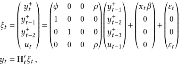
Our next step was to test if the potential candidates satisfy some desired statistics requirements (second condition). First, we test if the variables have the same integration order of GDP. Results are summarized inTable 2.
Based on the results of the Augmented Dickey-Fuller (ADF) test inTable 2, we do not reject the null hypothesis that the series areI(1), which makes us conclude that all analyzed time series have the same integration order of GDP. Next, we apply first differences to all these series and compute the correlation between each first-differenced series and first-differenced GDP, which is reported inTable 3.3 All the
analyzed series show a high correlation with the GDP series once both are first-differenced, although
3We have to aggregate the monthly series in order to compute correlation coefficients. We also compute correlations using
Table 2.ADF Unit Root Test.
Variables H0:zisI(1) H0:zisI(2)
GDP* −0.898 −4.098
[0.95] [0.01]
Steel −0.792 −5.514
[0.82] [0.00]
Vehicles 0.522 −6.208
[0.99] [0.00]
Cement −0.220 −3.392
[0.93] [0.01]
Energy −0.208 −26.672
[0.93] [0.00]
IP 0.690 −6.270
[0.99] [0.00]
Sales −0.118 −6.156
[0.95] [0.00]
Notes: (i) All series are in logs. The specification of the test equation was chosen on the basis of the Schwarz Information Criterion; (ii) the asterisk ( * ) indicates that a linear trend was included in the test equation; (iii) figures in brackets arep-values.
the correlation of GDP with Industrial Production and Sales is higher than that of other series. This concludes the cyclical analysis of the auxiliary series.4
We also investigate the trend pattern between each candidate auxiliary series and GDP. First, we run
Johansen’s (1991) cointegration test in order to verify whether there is a long-run relationship between GDP and candidate auxiliary series. As expected, we found that all tested series have one common trend with GDP.5
Based on the series cycles high correlation and the existence of a cointegration relationship, we select Industrial Production and Sales, and possibly Cement Production as well. It is interesting to note that the traditionally Coincident Series used in business-cycles analysis are the best choices to our interpolation method what confirms their capacity to track very well the economic activity.
Table 3. Correlation Coefficients – GDP and Coincident Series.
Variables Cement Vehicles Steel Energy IP Sales
GDP 0.49 0.33 0.29 0.21 0.66 0.57
3.2. Evaluation Results
In this section we present the results of the Kalman-filter estimation for each model considered. Before estimation, all series have been seasonally adjusted using the X12 procedure. InTable 4, we present the estimated parameters and coefficients of the auxiliary variables.
4We also compute the correlation coefficient between each candidate series cycles (extracted by Hodrick-Prescott filter) and GDP
cycle. Results are very similar to those inTable 3.
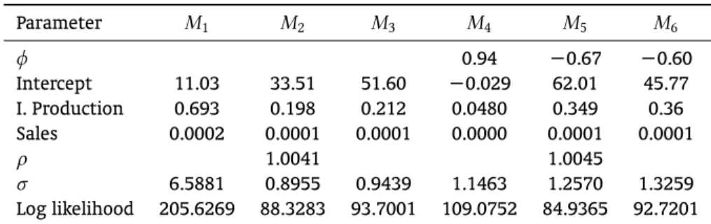
Table 4.Interpolation Results.
Parameter M1 M2 M3 M4 M5 M6
φ 0.94 −0.67 −0.60
Intercept 11.03 33.51 51.60 −0.029 62.01 45.77
I. Production 0.693 0.198 0.212 0.0480 0.349 0.36
Sales 0.0002 0.0001 0.0001 0.0000 0.0001 0.0001
ρ 1.0041 1.0045
σ 6.5881 0.8955 0.9439 1.1463 1.2570 1.3259
Log likelihood 205.6269 88.3283 93.7001 109.0752 84.9365 92.7201
Notes:(1) The models are described in the text and in theAppendix. (2) Industrial Production and Sales are used as auxiliary seriesxt.
From the results above we can see that the auxiliary coefficients and the estimated parameters change according to the model being estimated. In order to choose the model that best describe our GDP series, we make use of theR2measures of fit to gauge the accuracy of interpolation. InTable 5, we
present for each model, theR2measures of fit in first difference for the filtered and smoothed GDP.
With the exception of modelM1, all models have a highR2, so they show a reasonable interpolation
accuracy. The bestR2measure is obtained for ModelM2, followed by modelM3. Both impose thatρis
zero in (23). They only differ about the stochastic process of the error term: modelM2imposes that the
error is anAR(1)process, whereas modelM3imposes that it is ani.i.d.process.
ModelM2is a contemporaneously static model with anAR(1)error term. Taking first quasi-difference
of this model yields a restricted dynamic structure with one lag of dependent explanatory variables—the so calledcommon-factormodel:
(1−ρL)y+
t =(1−ρL)xtβ+(1−ρL)ut y+
t =ρyt+−1+xtβ−ρβxt−1+εt,
whereεt is white noise and there is an embedded restriction in the dynamic multipliers due to the
existence of a common factor.Figure 1depicts monthly and quarterly GDP, the former being estimated by ModelM2. The first graph shows the complete sample (1980–2012) while in the second one just the
recent period (1994–2012). Both show a smooth interpolated series, which fits closely to the observed quarterly series. Next, we investigate how well interpolated GDP behaves as compared to alternative GDP proxies available in Brazil.
Table 5.R2diffsMeasures of Fit. R2
diffs
Model GDP_filtered GDP_smoothed
M1 0.0273 0.0346
M2 0.4652 0.8097
M3 0.4382 0.7923
M4 0.3609 0.7098
M5 0.4011 0.5806
Figure 1.Monthly (Interpolated) and Quarterly (Observed) GDP.
60 80 100 120 140 160 180
94 96 98 00 02 04 06 08 10
Monthly GDP - Model 2 Quarterly GDP
60 80 100 120 140 160 180
1980 1985 1990 1995 2000 2005 2010
Monthly GDP - Model 2 Quarterly GDP
70
3.3. Comparing and evaluating the monthly GDP with other economic activity’s proxies
Monthly GDP estimated in last section could be widely used by practitioners and academics alike in-terested in measuring in real time the state of the economic activity. It also could be used to detect turning points in the Brazilian economy. In view of that, this section compares our monthly interpo-lated GDP with an alternative proxy of the economic activity recently constructed by the Central Bank of Brazil—the Brazilian Economic Activity Index (IBC-Br); seeBCB/Copom(2010), for example.6
IBC-Br is computed by aggregating monthly time-series from economy-wide supply-side sectors: agri-culture, industrial sector and services. In agriagri-culture, the source of information is the Systematic Survey of Agricultural Production released by IBGE. Regarding the industrial sector, IBC-Br monthly index is obtained by averaging the indices for four sub-sectors in our National Accounts, which are available on a monthly basis. They are weighted by value added at basic prices of the Quarterly National Accounts System in the previous year. Finally, the services sector includes time series from the trade activities, transportation, storage and mail services, financial intermediation, insurance, pension funds and re-lated services, real estate and rentals, management, public health and education and social security, and other services.
The first advantage of our monthly GDP over Br is computational. While putting together IBC-Br requires the aggregation of hundreds of monthly series, our interpolation method just requires the use of two covariate series in estimation. Second, IBC-Br methodology does not impose any restriction (discipline) between estimated levels vis-a-vis that of GDP or between estimated growth rates vis-a-vis that of GDP. In technical language, IBC-Br and GDP need not cointegrate and the cycles in IBC-Br and GDP growth rates need not be synchronized at the quarterly frequency. On the other hand, since our interpolated monthly GDP adds up to quarterly GDP for any given quarter, itmustdisplay the same short- and long-run behavior of observed GDP by construction, which is the great advantage of imposing discipline at the estimation level. Finally, because our estimate is based on a state-space representation, it can be immediately used tonowcastandforecastGDP,7as discussed in the previous section.
With these points in mind, we now compare these two economic activity proxies.Figure 2describes both series in levels while inFigure 3they are depicted in first differences. As can be seen, for the period 2005-12, the two series show a very similar trend pattern. However, this is not the case for their
6A detailed methodological description and the complete list of component time series could be found at Brazil’s Central Bank
homepage:http://www.bc.gov.br
7We should also mention that the IBC-Br series only begins in 2003, which prevents its use in business-cycle analysis, which
growth rates. For the latter, we time-aggregate both proxies of GDP at the quarterly frequency, and then compute their respective quarterly growth rates. These results are plotted inFigure 4. As expected, our estimated GDP proxy growth rate tracks that of quarterly GDP perfectly, which is not true regarding IBC-Br. We observe some larger discrepancies, especially in 2003-05 and 2007-08.
100 110 120 130 140 150
120 130 140 150 160 170
2005 2006 2007 2008 2009 2010 2011
IBC-Br
Kalman monthly GDP
Figure 2.IBC-Br and Kalman-Filter Monthly GDP (levels). -5 -4 -3 -2 -1 0 1 2 3 4
2005 2006 2007 2008 2009 2010 2011
IBC-Br
Kalman monthly GDP
Figure 3.IBC-Br and Kalman monthly GDP in first differences.
Figure 4.Quarterly Growth Rates of GDP, IBC-Br and Kalman-filter monthly GDP.
-6 -4 -2 0 2 4 6
1996 1998 2000 2002 2004 2006 2008 2010
Ëndice de Atividade Econ{mica S.A. (BC) Kalman GDP
Observed GDP
3.4. Detecting Business Cycles Turning Points
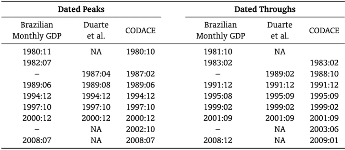
In this section, we first compute the chronology of business cycles (recessions vs. expansions) that is consistent with our monthly interpolated GDP, later comparing it with alternative business-cycle dat-ing’s, including that of the official Brazilian Business-Cycle Dating Committee (CODACE). Turning points are determined using the Bry and Boschan (1971) algorithm for detecting local minima and maxima of a time series. The dated turning points of Brazilian economic activity according to our interpolated GDP are presented below inFigure 5. InTable 6we make turning-point comparisons regarding alternative datings of Brazilian economic activity.
Figure 5.Monthly GDP – shaded by Bry Boshan recessions periods.
of the 1987–88 recession and of the 2002–03 recession. Our GDP dating misses these two episodes, while it keeps a very good record vis-a-vis CODACE’s datings, if we take into account the fact that the Brazilian Business-Cycle Dating Committee seems to have merged the 1980–81 recession with that of 1982–83.
Finally, we attempt here a historical account of Brazilian recessions according to our monthly GDP proxy. The recession in 1980–81 can be linked to the increase in interest rates by the FED in the early 1980s, which was later responsible for the emerging-market debt crisis (mostly in Latin America). The 1982–83 recession is related to the Latin American debt crisis itself, where international credit to these economies came to a halt after the Mexican moratorium in 1982. In these two recessions, there was an external factor at work.
Our next dated recession (1989–1991) was “home made,” which came as the result of the Brazilian government inability to curb high inflation with many unsuccessful economic plans. These all had in common the absence of long-term fiscal discipline, with an initial sudden transitory contraction of money supply.
After the Real Plan, in July 1994, inflation finally gets fairly under control and most recessions are again related to events abroad, which generated capital flight and thus prompted a sudden rise in do-mestic interest rates as a reaction to keep foreign capital in dodo-mestic markets. The Mexican crisis in
Table 6.Turning-Point Comparisons (Peaks and Throughs).
Dated Peaks Dated Throughs
Brazilian Monthly GDP
Duarte
et al. CODACE
Brazilian Monthly GDP
Duarte
et al. CODACE
1980:11 NA 1980:10 1981:10 NA
1982:07 1983:02 1983:02
– 1987:04 1987:02 – 1989:02 1988:10
1989:06 1989:08 1989:06 1991:12 1991:12 1991:12
1994:12 1994:12 1994:12 1995:08 1995:09 1995:09
1997:10 1997:10 1997:10 1999:02 1999:02 1999:02
2000:12 2000:12 2000:12 2001:09 2001:09 2001:09
– NA 2002:10 – NA 2003:06
1994 affected Brazil and other emerging markets. In 1997–98, the Asian, the Russian, and the Brazilian crises had similar effects here and in other emerging markets. On these occasions domestic interest rates had risen to very high levels, leading to a reduction in domestic economic activity. In 2000-02 our local energy-supply crisis—the rationing of electrical energy for consumers and industry—was respon-sible to an economy-wide contraction of economic activity, while in 2008-09 we had the global financial crisis with a short and limited contraction of Brazilian economic activity.
3.5. Nowcasting GDP
In this section we present evidence that one can indeed successfully nowcast Brazilian GDP using our interpolated monthly GDP. Here, we reproduce the results of the exercise inNotini et al.(2012). Instead of resorting to the techniques outlined insection 2.4, which rely on Kalman filtering, they performed a much simpler exercise, where the conditional nowcasting model is estimated by OLS and current observations of the covariates are used to nowcast GDP every month up to one quarter ahead. This quarterly forecast is then compared with the quarterly estimate of IBC-Br—the monthly GDP series put forth by the Central Bank of Brasil—in terms of its accuracy in forecasting actual quarterly GDP.
In their exercise,Notini et al.(2012) set the forecasting horizon to be one quarter. Hence, the GDP model forecasts three months ahead in order to nowcast quarterly GDP.Figure 6contains the results for this exercise, where the green line is the resulting error series transformed to growth rates. As can be seen below, apart from the beginning of 2009, the monthly GDP model nowcasts GDP with high accuracy.
Figure 6.Nowcast Errors of the Monthly GDP model.
-2% -1% -1% 0% 1% 1% 2%
-5% -3% -2% 0% 2% 3% 5%
Quarterly GDP Aggregated monthly Kalman GDP Dif (Dir.)
Next, we perform an out-of-sample forecast comparison between the monthly GDP model and IBC-Br. Notice that the latter is widely used by the banking industry to nowcast Brazilian GDP. It is important to note that there is no informational gap between our GDP nowcast and that of IBC-Br. So this is a fair nowcasting competition. Notini et al.(2012) compute the one-quarter ahead Mean Square Error (MSE) to assess the forecast accuracy of both forecasts. This is computed for two different periods: 2007:4 to 2011:4 and 2010:4 to 2011:4.Table 7summarizes the results.
Table 7.Nowcast Mean Squared Error – Monthly GDP Model Versus IBC-Br
Nowcast Period IBC-Br Monthly GDP Model
2007.4 – 2011.4 0.46% 0.40%
As can be seen fromTable 7, the monthly GDP model outperforms IBC-Br, and its superior perfor-mance is even stronger in the recent past, showing its usefulness in nowcasting Brazilian GDP. Further-more, we should expect the forecasting performance of the monthly GDP model to improve if we use kalman filtered coefficient estimates in nowcasting GDP instead of using OLS estimates.
4. CONCLUSIONS
In this paper, we propose an estimate for real monthly GDP in Brazil for the period 1980–2012, which is an interpolation of the quarterly observed series; seeBernanke et al.(1997) andMönch & Uhlig(2005). Our monthly GDP proxy is based on a state-space representation which imposes the restriction (disci-pline) that the monthly proxy adds up to quarterly observed GDP within every single quarter. A key issue is the choice of covariates used in interpolating the quarterly series: we chose to employ Indus-trial Production and Sales (corrugated paper sales) as covariates in interpolation, since these two series are key in Brazilian business-cycle analysis; seeDuarte et al.(2004) andIssler, Notini, & Rodrigues(2013).
The methodology inBernanke et al.(1997) andMönch & Uhlig(2005), allows estimating six different interpolation models, some of which have a long tradition in the literature. We are able to assess the fit of different models and related series in order to get the most appropriate monthly real GDP estimate: we evaluate six competing models, and six competing coincident series (Energy Demand, Steel Production, Cement Production, Vehicles Production, Industrial production and Sales), all available at the monthly frequency for the period 1980–2012.
First, we identify the series which behavior is closer to that of GDP, selecting Industrial Production and Sales. Second, we select the state-space model that has the highest goodness-of-fit statistic vis-a-vis GDP. We chose a contemporaneously static model with anAR(1) error term—which implies a restricted dynamic structure with one lag of dependent an explanatory variables. This best model is then estimated using Industrial Production and Sales as covariates yielding a smoothed estimate of Brazilian monthly GDP which serves as our GDP monthly proxy.
Next, we perform several interesting empirical exercises: we compare our GDP monthly proxy with alternative proxies available for Brazil. Our main comparison is regarding IBC-Br—the monthly GDP proxy made available by the Central Bank of Brazil. We discuss the advantages of our approach vis-a-vis theirs; we (re)establish a chronology of recessions in the recent past of the Brazilian economy using our GDP proxy. Its dating of recessions and expansions is compared with those ofDuarte et al.(2004) and to those of the Brazilian Business-Cycle Dating Committee (CODACE), showing a close enough dating; we also present the results of an out-of-sample nowcasting exercise using the monthly GDP model. Finally, its forecast accuracy in forecasting actual quarterly GDP is compared with that of the quarterly estimate of IBC-Br. From 2007:4 to 2011:4, its mean-squared error is 13% smaller than that of IBC-Br, whereas, for the recent past, 2010:4 to 2011:4, it is more than 50% smaller, showing its usefulness in nowcasting Brazilian GDP.
REFERENCES
BCB/Copom (2010). Índice de Atividade Econômica do Banco Central (IBC-Br). InRelatório de Inflação, Vol.12 No.1, 24–28. Brasília–DF: Banco Central do Brasil. Retrieved fromhttp://www.bcb.gov.br/?RELINF201003
Bernanke, B. S., Gertler, M., & Watson, M. (1997).Systematic monetary policy and the effects of oil price shocks
(Brookings Papers in Economic Activity No. 1). Washington, DC: Brookings Institution. Retrieved from
http://www.brookings.edu/about/projects/bpea/papers/1997/effects-of-oil-price-shocks-bernanke
Burns, A. F., & Mitchell, W. C. (1946).Measuring business cycles. New York: National Bureau of Economic Research (NBER).
Cardoso, E. A. (1981). Uma equação para a demanda de moeda no Brasil. Pesquisa e Planejamento Econômico,
Chauvet, M. (1998). An econometric characterization of business cycle dynamics with factor structure and regime switching.International Economic Review,39(4), 969–996. doi:10.2307/2527348
Chauvet, M. (2001). A monthly indicator of Brazilian GDP.Brazilian Review of Econometrics,21(1), 1–48. Retrieved fromhttp://bibliotecadigital.fgv.br/ojs/index.php/bre/article/view/3191
Chauvet, M. (2002). The Brazilian business and growth cycles.Revista Brasileira de Economia,56(1), 75–106. doi:
10.1590/S0034-71402002000100003
Chow, G. C., & Lin, A.-l. (1971). Best linear unbiased interpolation, distribution, and extrapolation of time series by related series.The Review of Economics and Statistics,53(4), 372–375. doi:10.2307/1928739
Contador, C. R. (1977).Ciclos econômicos e indicadores de atividade no Brasil(Relatório de pesquisa No. 35). Rio de Janeiro: Instituto de Planejamento Econômico e Social / Instituto de Pesquisas (IPEA/INPES).
Contador, C. R., & Ferraz, C. (1999).Previsão com indicadores antecedentes. Rio de Janeiro: Silcon.
Contador, C. R., & Santos Filho, W. A. C. d. (1987). Produto Interno Bruto trimestral: bases metodológicas e estimativas.Pesquisa e Planejamento Econômico,17(3), 711–742.
Cuche, N. A., & Hess, M. K. (2000). Estimating monthly GDP in a general Kalman filter framework: Evidence from Switzerland.Economic and Financial Modelling,7(4), 153–194.
Duarte, A. J. M., Issler, J. V., & Spacov, A. (2004). Indicadores coincidentes de atividade econômica e uma cronologia de recessões para o Brasil.Pesquisa e Planejamento Econômico,34(1), 1–37.
Fernández, R. B. (1981). A methodological note on the estimation of time series. The Review of Economics and Statistics,63(3), 471–476. doi:10.2307/1924371
Giannone, D., Reichlin, L., & Small, D. (2008). Nowcasting: The real-time informational content of macroeconomic data.Journal of Monetary Economics,55(4), 665–676. doi:10.1016/j.jmoneco.2008.05.010
Hamilton, J. D. (1994).Time series analysis. Princeton, NJ: Princeton University Press.
Harvey, A. C. (1989). Forecasting, structural time series models and the Kalman Filter. Cambridge University Press.
Hollauer, G., Issler, J. V., & Notini, H. H. (2009). Novo indicador coincidente para a atividade industrial brasileira.
Economia Aplicada,13(1), 5–28. doi:10.1590/S1413-80502009000100001
Issler, J. V., Notini, H. H., & Rodrigues, C. F. (2013). Constructing coincident and leading indices of economic activity for the Brazilian economy. Journal of Business Cycle Measurement and Analysis,2012(2), 43–65. doi:
10.1787/19952899
Issler, J. V., Notini, H. H., Rodrigues, C. F., & Soares, A. F. (2013). Constructing coincident indices of economic activity for the Latin American economy.Revista Brasileira de Economia,67(1), 67–96. doi: 10.1590/S0034-71402013000100004
Issler, J. V., & Spacov, A. D. (2000). Usando correlações canônicas para identificar indicadores antecedentes e coincidentes da atividade econômica no Brasil(Relatório de Pesquisa – mimeo). Ministério da Fazenda. Issler, J. V., & Vahid, F. (2006). The missing link: Using the NBER recession indicator to construct
co-incident and leading indices of economic activity. Journal of Econometrics, 132(1), 281–303. doi:
10.1016/j.jeconom.2005.01.031
Johansen, S. (1991). Estimation and hypothesis testing of cointegration vectors in Gaussian vector autoregressive models.Econometrica,59(6), 1551–1580. doi:10.2307/2938278
Kim, C.-J., & Nelson, C. (1999, Sep). A bayesian approach to testing for Markov switching in univariate and dynamic factor models(Discussion Paper No. 0035). University of Washington, Department of Economics. Liu, H., & Hall, S. G. (2001). Creating high-frequency national accounts with state-space modelling: a Monte Carlo
experiment.Journal of Forecasting,20(6), 441–449. doi:10.1002/for.810
Mariano, R. S., & Murasawa, Y. (2003). A new coincident index of business cycles based on monthly and quarterly series.Journal of Applied Econometrics,18(4), 427–443. doi:10.1002/jae.695
Mitchell, T. D., & Jones, P. D. (2005). An improved method of constructing a database of monthly climate obser-vations and associated high-resolution grids. International Journal of Climatology,25(6), 693–712. doi:
10.1002/joc.1181
Nakane, M. I. (1994).Testes de exogeneidade fraca e de superexogeneidade para a demanda por moeda no Brasil. Rio de Janeiro: BNDES.
Notini, H., Issler, J. V., Rodrigues, C., Matos, S., , & Bonelli, R. (2012). Nowcasting Brazilian monthly GDP: A state-space approach [paper presented at CIRET 2012, Vienna].
Picchetti, P., & Toledo, C. (2002). Estimating and interpreting a common stochastic component for the Brazil-ian Industrial Production Index. Revista Brasileira de Economia,56(1), 107–120. doi: 10.1590/S0034-71402002000100004
Spacov, A. D. (2001). Índices antecedentes e coincidentes da atividade econômica brasileira: Uma aplicação da análise de correlação canônica(Dissertação de Mestrado). Fundação Getúlio Vargas, Escola de Pós-Graduação em Economia (FGV/EPGE), Rio de Janeiro.
Stock, J. H., & Watson, M. W. (1988, November). A probability model of the coincident economic indicators
(Working Paper No. 2772). National Bureau of Economic Research (NBER). doi:10.3386/w2772
Stock, J. H., & Watson, M. W. (1989). New indexes of coincident and leading economic indicators. In O. J. Blanchard & S. Fischer (Eds.),NBER Macroeconomics Annual 1989, volume 4(pp. 351–409). MIT Press. Retrieved from
http://www.nber.org/chapters/c10968
Stock, J. H., & Watson, M. W. (1991). A probability model of the coincident economic indicator. In K. Lahiri & G. H. Moore (Eds.),Leading economic indicators: New approaches and forecasting records(pp. 63–89). Cambridge University Press.
Stock, J. H., & Watson, M. W. (Eds.). (1993a).New research on business cycles, indicators and forecasting. Univer-sity of Chicago Press.
Stock, J. H., & Watson, M. W. (1993b). A procedure for predicting recessions with leading indicators: Economet-ric issues and recent experience. In J. H. Stock & M. W. Watson (Eds.),New research on business cycles, indicators and forecasting.University of Chicago Press.
Stock, J. H., & Watson, M. W. (2002a). Forecasting using principal components from a large number of predictors.
Journal of the American Statistical Association,97(460), 1167–1179. doi:10.1198/016214502388618960
Stock, J. H., & Watson, M. W. (2002b). Macroeconomic forecasting using diffusion indexes.Journal of Business & Economic Statistics,20(2), 147–162. doi:10.1198/073500102317351921
APPENDIX. DETAILED INTERPOLATION MODELS
The literature appoint as the main problem of the modelsM1andM2is the fact that they extract signals
only from the presumed stochastic process of the original series in a way that no new information is added. We believe that we would be better off enriching the model with additional information contained in the related series.
ModelM1
This is the simpler model which incorporates information from related series. So it can be used as a benchmark when we estimate the more sophisticated models. It can be stated as:
yt=xt′β+ϵt
where:xt′is a vector of related series andϵt a iid error term with distributionN(0,σ2).
ModelM2
This is theChow & Lin(1971) model. This model is very used in the literature because they are the first to show how to include related series in the interpolation procedure. They suggest a regression model without lagged dependent variables, but autoregressive errors, so we can obtain theChow & Linmodel by fixingφ=0and by lettingρto be estimated freely:
εt= *. .. .. , yt yt−1
yt−2
ut +/ // // -= *. .. .. ,
0 0 0 ρ
1 0 0 0
0 1 0 0
0 0 0 ρ
+/ // // -*. .. .. ,
yt−1
yt−2
yt−3
ut−1
+/ // // -+ *. .. .. , x′ tβ 0 0 0 +/ // // -+ *. .. .. , ϵt 0 0 ϵt +/ // // -y+ =h′tεt
It is important to note that in their seminal paper,Chow & Lindo not use the Kalman filter but it can be shown that the Kalman filter above and theChow & Linregression yield the same estimates by maximum likelihood (Cuche & Hess,2000).
ModelM3
This is a variation of theChow & Linmodel, suggested byFernández(1981), where instead of the regres-sion ofytin levels, it uses the first differences ofytin order to account for non-stationarity. This model is obtained by letting regression residuals to be a random walk, i.e.φ=0andρ=1.
ModelM4
This model was suggested byMitchell & Jones(2005) and it is a dynamic version of modelM1.
ModelM5
A modified version of modelM4 where we impose thatρ=1.
ModelM6
It is the most general version of theMitchell & Jones(2005) model, where we letφandρto be estimated
freely.
![Table 2. ADF Unit Root Test. Variables H 0 : z is I (1) H 0 : z is I (2) GDP* −0.898 −4.098 [ 0.95 ] [ 0.01 ] Steel −0.792 −5.514 [ 0.82 ] [ 0.00 ] Vehicles 0.522 −6.208 [0.99] [0.00] Cement −0.220 −3.392 [0.93] [0.01] Energy −0.208 −26.672 [0.93] [0.00] I](https://thumb-eu.123doks.com/thumbv2/123dok_br/18916412.433662/10.850.285.544.160.453/table-unit-root-variables-steel-vehicles-cement-energy.webp)