ISSN 0101-8205 / ISSN 1807-0302 (Online) www.scielo.br/cam
The Poisson-exponential regression model under
different latent activation schemes
FRANCISCO LOUZADA1∗, VICENTE G. CANCHO1 and GLADYS D.C. BARRIGA2
1SME, ICMC – Universidade de São Paulo, São Carlos, São Paulo, Brasil 2FEB – Universidade Estadual Paulista
E-mails: [email protected] / [email protected] / [email protected]
Abstract. In this paper, a new family of survival distributions is presented. It is derived by
considering that the latent number of failure causes follows a Poisson distribution and the time for these causes to be activated follows an exponential distribution. Three different activation schemes are also considered. Moreover, we propose the inclusion of covariates in the model formulation in order to study their effect on the expected value of the number of causes and on the failure rate function. Inferential procedure based on the maximum likelihood method is discussed and evaluated via simulation. The developed methodology is illustrated on a real data set on ovarian cancer.
Mathematical subject classification: 62N01, 62N99.
Key words: activation schemes, exponential distribution, poisson distribution, survival
analysis.
1 Introduction
As well known, although the exponential distribution provides a simple, ele-gant and close form solution to many problems in lifetime testing and reliability studies, it does not provide a reasonable parametric fit for some practical ap-plications where the underlying failure rates are nonconstant, presenting mono-tone shapes. In recent years, in order to overcame such problem, new classes
of models were introduced based on modifications of the exponential distribu-tion. Gupta and Kundu (1999) proposed a generalized exponential distribution, this family can accommodate data with increasing and decreasing failure rate function. Adamidis and Loukas (1998) introduced the exponential-geometric distribution with decreasing failure rate. Ku¸s (2007) proposed a two-parameter distribution known as exponential-Poisson distribution, which has decreasing failure rate. Tahmasbi and Rezaei (2008) proposed another modification of the exponential distribution with decreasing failure rate function. This distribution is known as logarithmic-exponential distribution. Cancho et al. (2011) introduced the Poisson-exponential distribution with increasing failure rate. This model is derived in a complementary risks scenario (Louzada-Neto, 1999), where the lifetime associated with a particular risk is not observable, rather we observe only the maximum lifetime value among all risks.
In this paper we proposed a class of hierarchical models with latent compet-ing risks and different activation schemes, where the lifetime associated with a particular risk is not observable, rather we observe only the minimum, maxi-mum or a randomly lifetime value among all risks, with the lifetimes following an exponential distribution. We consider, that the number of latent competing risks (or causes) is modeled by a zero truncated Poisson distribution, with our formulation has several particular cases, including the models proposed by Ku¸s (2007) and Cancho et al. (2011).
The paper is organized as follows. In Section 2, we introduce the new dis-tribution and present its properties. Section 3 we carry out inference for the Poisson-exponential regression model, discuss some measures of model selec-tion. Section 4 we present the results of a simulation study and in Section 5 the methodology is illustrated on a real ovarian cancer data set. Some final comments are presented in Section 6.
2 The model
LetMdenote the unobservable number of causes related to the occurrence of an event of interest for an individual in the population. Assume thatM has a zero truncated Poisson distribution with probability mass function given by
P(M=m)= pm =
e−θθm
The time for the jth cause to produce the event of interest is denoted by Tj,
j = 1, . . . ,M. We assume that, conditional on M, the Tj are independent
and identically distributed with cumulative distribution function G(t). Also, we assume that T1, T2, . . . are independent of M. Further, consider the order statistics of theTj’s,T(1) ≤ T(2), . . . ,T(R) ≤. . .≤T(M). The observed lifetime
can be defined by the random variable Y = T(R), where R = 1,2, . . . ,M is
dependent ofM. In many biological process, Rindicates the resistance factor of the immune system of the individual. In other words, as in Cooner et al. (2007), R out of N causes are required to produce the event of interest. The resistance factor can be a fixed constant, a function of Mor a random variable specified through a conditional distribution onM.
In this paper we deal with three specifications for R. Firstly, we assume that given M, the conditional distribution of R is uniform on {1,2, . . . ,M} (random activation scheme). Under this setup, the distribution function forY givenM=mandR =r, is given by
FY|m,r(y)= P[Y ≤ y|M =m,R=r]
=
m
X
j=r
m
j
(G(y))j(1−G(y))m−j. (2)
Also, we can demonstrate that the marginal distribution function ofY is given by
Frandom(y)=
∞ X
m=1
m
X
r=1
P[T(R)≤ y|M =m,R =r)]
×P[R =r|M =m]P[M=m] =1−
∞ X
m=1
( m
X
r=0
(m−r)B(r,m,G(y)) )
1 mpm
=1−(1−G(y)) ∞ X
m=1
pm =G(y),
(3)
Note that, in (3), the distribution function ofY is the same as the distribution of the latent random variablesTj’s. If we consider that R =r (fixed), then the
marginal distribution ofY is given
F(y)=
∞ X
m=1
I B(F(y);r,m−r +1)pm
=
∞ X
m=1 m
m−1 r −1
Z G(y)
0
ur−1(1−u)m−rdu pm,
(4)
whereI B(x;a,b)is incomplete beta function and pmis given in (1).
As a second setup, the so-called first activation scheme (Cooner et al., 2007), we suppose that the event of interest happens due to any one of the possible causes, but for R =1. Then, the observed failure isY = Z(1) = min{T1, . . . ,TM}. In
this case the marginal distribution ofY in (4) is given by Ffirst(y)= 1−e
−θG(y)
1−e−θ , y >0. (5)
In a third scenario, also known as the last activation scheme (Cooner et al., 2007), the event of interest only takes place after all the M causes have been occurred, so that R = M and the observed failure time is Y = Z(M) =
max{T1, . . . ,TM}. The marginal distribution ofY in (4)is given by
Flast(y)= e
−θ (1−G(y))−e−θ
1−e−θ , y >0. (6)
The relationship between the distribution functions in (3), (5) and (6) is described in next proposition.
Proposition 2.1. Under some conditions on the models in(3),(5)and(6), for any distribution function G(y), Flast(y)≤ Frandom(y)≤ Ffirst(y) for y>0.
Proof. We know that A(y) = 1−e−θG(y)
G(y) is a decreasing function iny, indeed,
let
B(y)=θG(y)e−θG(y)+e−θG(y)−1,
and limy→0B(y)=0 thusB(y) <0, ∀y. So
A′(y)= g(y)[θG(y)e
−θG(y)+e−θG(y)−1]
G(y)2 =
g(y)B(y)
G(y)2 <0, ∀y>0, and as
lim
y→∞A(y)=
1−e−θG(y)
G(y) =1−e −θ
,
then,
1−e−θG(y)
G(y) ≥1−e
−θ, ∀y, i.e., 1−e−θG(y)
1−e−θ ≥G(y), ∀y.
Similarly, we can prove theFlast(y)≤ Fr andom(y) ∀y.
Considering different choices for the distribution of latent random variables Tj’s, new families of distribution can be obtained. For instance, the
exponential-Poisson distribution proposed by Ku¸s (2007) is obtained by considering that the variable Tj’s follows an exponential distribution with failure rate
func-tion, λ > 0, under the first-activation scheme, members of this family of distribution have decreasing failure rate functions. For properties of this dis-tribution interested readers can refer to Ku¸s (2007). The counterpart distribu-tion is proposed by Cancho et al. (2011), with observed time failure given by Y = max(Z1, . . . ,ZM) (last-activation), which has increasing failure rate
function.
We may consider an extension of the exponential-Poisson (EP) models un-der latent competitive risks and different activation schemes, by including co-variates in the modeling. Particularly, in order to study the effect of covari-ates on the value expected of number of causes (E(M) = η), we change the parametrization of the models in (5) and (6) in order to include E(M) = η
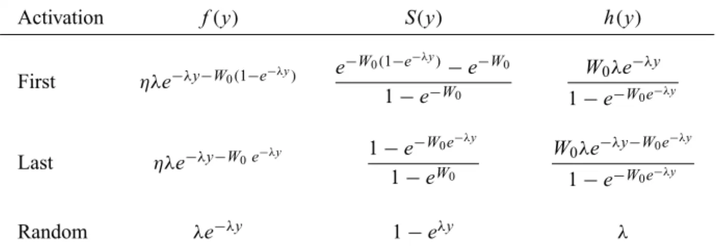
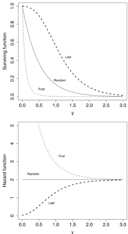
In this context, we obtain the survival, failure rate and density functions presented in Table 1 for the unobserved failure time T following exponential distribution with failure rateλ > 0. Figure 1 portrays distinct behaviors of the survival functions (top panel) and the failure rate functions (bottom panel) in Table 1. These plots illustrate the flexibility afforded by our proposal.
Activation f(y) S(y) h(y)
First ηλe−λy−W0(1−e−λy) e
−W0(1−e−λy)−e−W0 1−e−W0
W0λe−λy
1−e−W0e−λy
Last ηλe−λy−W0e−λy 1−e
−W0e−λy 1−eW0
W0λe−λy−W0e−λy 1−e−W0e−λy
Random λe−λy 1−eλy λ
Remark.W0=η+ W(−ηe−η), whereW(∙)is the LambertWfunction (Corless et al., 1996).
Table 1 – Survival function(S(y)), hazard function(h(y))and density function(f(y))
for exponential-Poisson under different activation schemes.
3 Inference
Let us consider the situation when the failure timeY in Section 2 is not com-pletely observed and it is subjected to right no-informative censoring. Let Ci
denote the censoring time. In a sample of sizen, we then observe ti =min{Yi,Ci} and δi =I(Yi ≤Ci),
where δi = 1 if Ti is a failure time and δi = 0 if it is right censored, for
i=1, . . . ,n.
Let xi and zi denote the covariate vector. We relate the model parameters η
andλto covariates xi andzi by adopting the following link functions,
log(ηi)=xi⊤β and log(λi)=z⊤i γ, (7)
i = 1, . . . ,n, where β and γ denote vectors of coefficients, and xi and zi
Figure 1 – Top panel: Survival function of the PE distribution. Bottom panel: Failure rate function of the PE distribution. Withη=6 andλ=2.
With the expression (7) we can write the likelihood ofϑ =(β⊤,γ⊤)⊤under right non-informative censoring as
L(ϑ;D)∝
n
Y
i=1
f(ti;ϑ)δi S(ti;ϑ)1−δi, (8)
where D = (t,δ,x,z), t = (t1, . . . ,tn)⊤ and δ = (δ1, . . . , δn)⊤, whereas
From the likelihood function in (8), the maximum likelihood estimation of the parameterϑ is carried out. Numerical maximization of the log-likelihood functionℓ(ϑ) = logL(ϑ;D) is accomplished by using existing software. In this paper, the software R (see, R Development Core Team, 2009) was used to compute maximum likelihood estimates (MLE). The Lambert W function in Table 1 can be found in the R package emdbook. Covariance estimates for the maximum likelihood estimatorsbϑ may also be obtained using the Hessian matrix. For large samples, confidence intervals may be conducted by using the large sample distribution of the MLE which is a normal distribution with the covariance matrix as the inverse of the Fisher information. More specifically, the asymptotic covariance matrix is given byI−1(ϑ) with I(ϑ) = −E[J(ϑ)] such thatJ(ϑ)=∂2ℓ(ϑ)/∂ϑ∂ϑT.Since it is not possible to compute the Fisher information matrixI(ϑ)due to the censored observations (censoring is random and non-informative), it is possible to use the matrix of second derivatives of the log likelihood,−J(ϑ), evaluated at the MLEϑ =bϑ, which is a consistent estimator. The required second derivatives are computed numerically.
Besides estimation, hypothesis testing is another key issue. Let ϑ1 andϑ2 be two proper disjoint subsets of ϑ. We aim to test H0 : ϑ1 = ϑ01 against H1:ϑ16=ϑ01,ϑ2unspecified. Letϑˆ0maximizeL(ϑ;D)constrained toH0and define the log-likelihood ratio statistic aswn =2
ℓ(ϑˆ)−ℓ(ϑˆ0)
, whereℓ(∙)is the log-likelihood. Under H0 and some regularity conditions,wn converges in
distribution to a chi-square distribution with dim(ϑ1) degrees of freedom. Different models can be compared penalizing over-fitting by considering the Akaike information criterion given byAI C = −2ℓ(bϑ)+2#(ϑ)and the Schwartz information criterion defined by S I C = −2ℓ(bϑ)+#(ϑ)log(n), where #(ϑ)is the number of model parameters. The model with the smallest value of any of these criteria (among all models considered) is commonly taken as the preferred model for describing the dataset.
4 Simulation
the Poisson-exponential regression model with increasing failure rate function (first-activation) with two covariates, xi and zi, being that, xi generated from
a Bernoulli distribution with parameter 0.5 and zi generated from a uniform
distribution on the range [0,1]. The failure times were simulated from the quantile function of model (via the inversion method) with parameter ηi =
exp(β10 +β11xi) and λi = exp(β20 +β21zi), where β = (1,1) and γ =
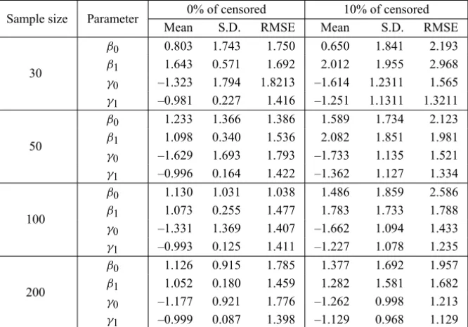
(−1,−1). Censoring time were generated from an uniform distribution[0, τ], whereτ controlled the proportion of censoring, which is considered here equals to 0% and 10%. We considered sample sizesn equal to 30,50,100 and 200. For each configuration, we conducted 1,000 replicates and then we averaged the estimates of the parameters, the standard errors and the square root of the mean square errors.
The Table 2 show that the bias of the MLEsβandθ, and their standard errors and root mean squared errors become smaller when the sample size increases and the percentage of censored observations is smaller.
0% of censored 10% of censored Sample size Parameter
Mean S.D. RMSE Mean S.D. RMSE
30
β0 0.803 1.743 1.750 0.650 1.841 2.193
β1 1.643 0.571 1.692 2.012 1.955 2.968
γ0 –1.323 1.794 1.8213 –1.614 1.2311 1.565
γ1 –0.981 0.227 1.416 –1.251 1.1311 1.3211
50
β0 1.233 1.366 1.386 1.589 1.734 2.123
β1 1.098 0.340 1.536 2.082 1.851 1.981
γ0 –1.629 1.693 1.793 –1.733 1.135 1.521
γ1 –0.996 0.164 1.422 –1.362 1.127 1.334
100
β0 1.130 1.031 1.038 1.486 1.859 2.586
β1 1.073 0.255 1.477 1.783 1.733 1.788
γ0 –1.331 1.369 1.407 –1.662 1.094 1.433
γ1 –0.993 0.125 1.411 –1.227 1.078 1.235
200
β0 1.126 0.915 1.785 1.377 1.692 1.957
β1 1.052 0.180 1.459 1.282 1.581 1.682
γ0 –1.177 0.921 1.776 –1.262 0.998 1.213
γ1 –0.999 0.087 1.398 –1.129 0.968 1.129
5 Application
In this section we reanalyze the data extracted from Collett (2003). The data describe a study of 26 women diagnosed with ovarian cancer submitted to chemotherapy. The data consist of the survival times yi (in months) of patients
and several prognostic covariates such as: x1i: treatment (0=single, 1=
com-bined),x2i: age of patient in years, x3i: extent of residual disease (0 =
incom-plete, 1=complete) andx4i: performance status (0=good, 1=poor).
Firstly, in order to identify the shape of a lifetime data failure rate function we shall consider, as a crude indicative, a graphical method based on the TTT plot (Aarset, 1985). In its empirical version the TTT plot is given by
G(r/n)=
h Pr
i=1Yi:n
+(n−r)Yr:n
i
Pr
i=1Yi:n
,
wherer = 1, . . . ,nandYi:n represent the order statistics of the sample. It has
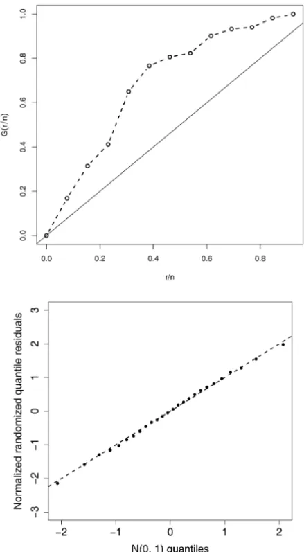
been shown that the failure rate function is increasing (decreasing) if the TTT plot is concave (convex). Figure 2 (top panel) shows the TTT plot for the consid-ered data, which is concave indicating an increasing failure rate function, which can be properly accommodated by a Poisson-exponential regression model with increasing failure rate. This proposal indicates that all causes were responsible for activating the event of interest (last-activation scheme).
Firstly, we consider the following EP regression model with all covariates, i.e,
log(ηi)=β0+β1x1i+β2x2i +β3x3i+β4xii,
and
log(λi)=γ0+γ1x1i+γ2x2i +γ3x3i+γ4x4i, i =1, . . . ,26,
Table 3 presents the MLEs of the coefficients. The QQ plot of the normalized randomized quantile residuals (Dunn and Smyth, 1996; Rigby and Stasinopou-los, 2005) in Figure 2 (bottom panel) suggests that the Poisson-exponential regression model yields an adequate fit. Each point in Figure 2 (bottom panel) corresponds to the median of ten sets of ordered residuals.
Figure 2 – Top panel: Empirical scaled TTT-Transform for the data. Bottom panel: QQ plot of the normalized randomized quantile residuals with identity line for the REP model each point corresponds to the median of ten sets of ordered residuals.
2.18, with g.l =6 and p-value= 0.902, indicating that the effect coefficients are no significant in the model. Thus, the final Poisson-exponential regression model becomes the one given by
Parameter Estimate (est) Standard error (se) |est|/ se
β0 2.130 2.585 0.824
β1(treatment) 0.787 1.104 0.713
β2(age) –0.010 0.050 0.200
β3(residual) –0.574 1.240 0.463
β4(performance) 0.700 1.378 0.509
γ0 –6.345 1.898 3.344
γ1(treatment) –0.013 0.604 0.0207
γ2(age) 0.066 0.036 1.893
γ3(residual) 0.069 0.622 0.111
γ4(performance) 0.517 0.804 0.643
Table 3 – MLEs for the parameters of the Poisson-exponential regression model.
Parameter Estimate (est) Standard error (se) |est|/ se
β0 1.283 0.482 2.658
β1(treatment) 0.950 0.485 1.960
γ0 –7.171 1.315 –5.452
γ2(age) 0.084 0.020 4.237
Table 4 – Maximum likelihood estimates for the final model.
Table 4 shows the MLEs and their standard errors of the parameters for final Poisson-exponential regression model. We note the covariatetreatmentis signif-icant (at 5%) for the expected value of number of causes, while that the covariate ageis significant (at 1%) in the failure rate.
Figure 3 – Top panel: Surviving function of REP model. Bottom panel: Failure rate function of REP model.
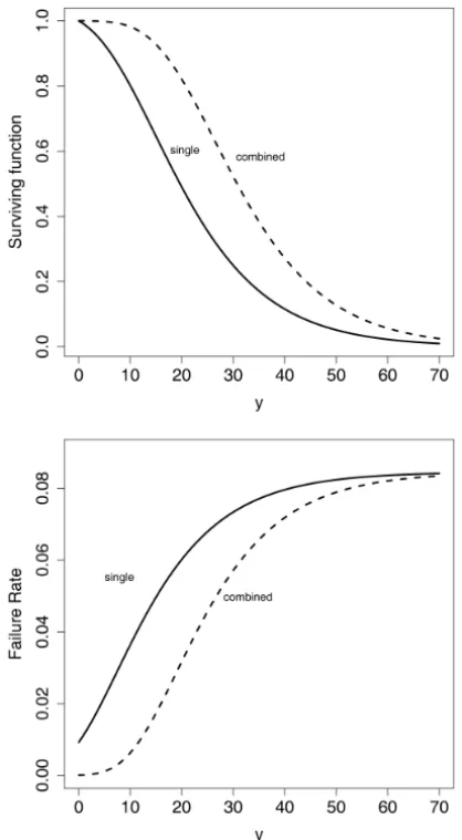
The benefit of thecombining treatmentcan be observed from Figure 3, which displays the surviving (top panel) and failure rate (bottom panel) functions for 56 years old (age mean) patients stratified bytreatment, implying in an increas-ing in survival and a decreasincreas-ing in failure rate when thecombining treatmentis used instead of considering thecontrol treatment.
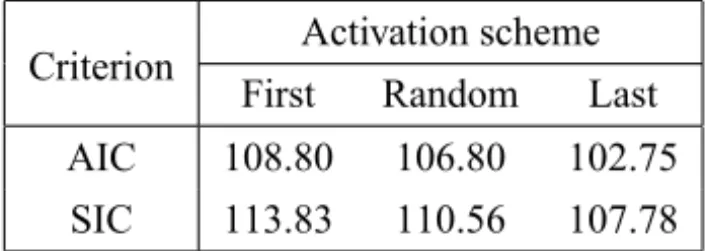
above, for sake of comparison we fitted the Poisson-exponential regression model under the other two activation schemes, namely, first and random ac-tivation schemes. We fitted these models with the same covariates as to our final model (see Table 4). The estimated AIC and SIC for the models are reported in the Table 5. Notice that the Poisson-exponential regression model under the last activation scheme outperforms the other two schemes irrespective of the criterion considered. Finally, we fitted the usual Weibull regression model, with AIC and SIC values equals to 103.90 and 108.93, respectively, which also was outper-formed by our Poisson-exponential regression model under the last activation scheme.
Activation scheme Criterion
First Random Last
AIC 108.80 106.80 102.75
SIC 113.83 110.56 107.78
Table 5 –AI CandS I Ccriterion values for the adjusted Poisson-exponential regression model under first, random and last activation schemes.
6 Concluding remarks
In this paper we proposed the Poisson-exponential regression model, as a possi-ble extension of the well known exponential regression model. The model was built based on a latent competing risk structure with three different activation schemes, minimum, maximum or random. We discussed parameter maximum likelihood estimation and a straightforwardly modeling comparison procedure. The flexibility of our modeling was illustrated in on a real data set on ovarian cancer.
Ku¸s (2007) and Tahmasbi and Rezaei (2008) by compounding an exponential distribution and power series distribution, but they only considered a minimum activation scheme. A possible study involving the power series distribution in the context of our modeling with three different activation schemes shall be considered elsewhere.
Models for survival data with a surviving fraction take a prominent position in survival studies, covering situations where there are sampling units insuscep-tible to the occurrence of the event of interest (Rodrigues et al., 2009; Louzada et al., 2011; Perdona and Louzada, 2011). The proposed Poisson-exponential regression model for survival data in presence of a survival fraction should be considered in a future study, as well as modeling considering the shape parameter depending on covariates (Louzada-Neto, 1997). Diagnostic methods have been an important tool in survival regression analysis. Influential diagnostics should be investigated further in the context of the proposed Poisson-exponential re-gression model (Fachini et al., 2008).
Acknowledgments. The authors are grafeful the Editorial Boarding as well as to the referees for their comments and suggestions. The research of Francisco Louzada and Vicente G. Cancho are funded by the Brazilian organization CNPq.
REFERENCES
[1] M.V. Aarset,The null distribution for a test of constant versus “bathtub” failure rate.Scandinavian Journal of Statistics,12(1) (1985), 55–68.
[2] K. Adamidis and S. Loukas,A lifetime distribution with decreasing failure rate. Statistics & Probability Letters,39(1) (1998), 35–42.
[3] V. Cancho, F. Louzada-Neto and G. Barriga, The poisson-exponential lifetime distribution.Computational Statistics & Data Analysis,55(2011), 677–686.
[4] M. Chahkandi and M. Ganjali, On some lifetime distributions with decreasing failure rate.Comput. Stat. Data Anal.,53(12) (2009), 4433–4440.
[5] D. Collett, Modelling survival data in medical research. CRC press. ISBN 1584883251, (2003).
[7] R.M. Corless, G.H. Gonnet, D.E.G. Hare, D.J. Jeffrey and D.E. Knuth, On the Lambert W function.Advances in Computational Mathematics, 5(1996), 329– 359.
[8] P.K. Dunn and G.K. Smyth,Randomized quantile residuals.Journal of Computa-tional and Graphical Statistics,5(3) (1996), 236–244.
[9] J.B. Fachini, E.M.M. Ortega and F. Louzada-Neto, Influential diagnostics for polyhazard models in the presence of covariates.Statistical Methods and Appli-cations,17(2008), 413–433.
[10] R. Gupta and D. Kundu,Generalized exponential distributions.Australian and New Zealand Journal of Statistics,41(2) (1999), 173–188.
[11] D. Ku¸s, A new lifetime distribution distributions. Computational Statistics & Data analysis,11(2007), 4497–4509.
[12] F. Louzada, M. Roman and V. Cancho, The complementary exponential geo-metric distribution: Model, properties, and a comparison with its counterpart. Manuscript submitted to Computational Statistics & Data Analysis (2011).
[13] F. Louzada-Neto,Extended hazard regression model for reliability and survival analysis.Lifetime Data Analysis,3(1997), 367–381.
[14] F. Louzada-Neto, Poly-hazard regression models for lifetime data. Biometrics, 55(1999), 1121–1125.
[15] G.S.C. Perdona and F. Louzada,A general hazard model for lifetime data in the presence of cure rate.Journal of Applied Statistics,38(2011), 1395–1405.
[16] R Development Core Team,R: A Language and Environment for Statistical Com-puting.R Foundation for Statistical Computing, Vienna, Austria (2009).
[17] R.A. Rigby and D.M. Stasinopoulos,Generalized additive models for location, scale and shape (with discussion).Applied Statistics,54(3) (2005), 507–554.
[18] J. Rodrigues, V.G. Cancho, M. de Castro and F. Louzada-Neto,On the unifica-tion of the long-term survival models.Statistics & Probability Letters,79(2009), 753–759.