www.geosci-model-dev.net/8/1139/2015/ doi:10.5194/gmd-8-1139-2015
© Author(s) 2015. CC Attribution 3.0 License.
JULES-crop: a parametrisation of crops in the Joint UK Land
Environment Simulator
T. Osborne1, J. Gornall2, J. Hooker3, K. Williams2, A. Wiltshire2, R. Betts2,4, and T. Wheeler5
1National Centre for Atmospheric Science, University of Reading, Reading, UK 2Hadley Centre, Met Office, Exeter, UK
3Joint Research Centre, Ispra, Italy
4College of Life and Environmental Sciences, University of Exeter, Exeter, UK 5Department of Agriculture, University of Reading, Reading, UK
Correspondence to:J. Gornall ([email protected])
Received: 8 September 2014 – Published in Geosci. Model Dev. Discuss.: 14 October 2014 Revised: 19 March 2015 – Accepted: 20 March 2015 – Published: 22 April 2015
Abstract. Studies of climate change impacts on the terres-trial biosphere have been completed without recognition of the integrated nature of the biosphere. Improved assessment of the impacts of climate change on food and water security requires the development and use of models not only repre-senting each component but also their interactions. To meet this requirement the Joint UK Land Environment Simulator (JULES) land surface model has been modified to include a generic parametrisation of annual crops. The new model, JULES-crop, is described and evaluation at global and site levels for the four globally important crops; wheat, soybean, maize and rice. JULES-crop demonstrates skill in simulat-ing the inter-annual variations of yield for maize and soy-bean at the global and country levels, and for wheat for ma-jor spring wheat producing countries. The impact of the new parametrisation, compared to the standard configuration, on the simulation of surface heat fluxes is largely an alteration of the partitioning between latent and sensible heat fluxes dur-ing the later part of the growdur-ing season. Further evaluation at the site level shows the model captures the seasonality of leaf area index, gross primary production and canopy height better than in the standard JULES. However, this does not lead to an improvement in the simulation of sensible and la-tent heat fluxes. The performance of JULES-crop from both an Earth system and crop yield model perspective is en-couraging. However, more effort is needed to develop the parametrisation of the model for specific applications. Key future model developments identified include the introduc-tion of processes such as irrigaintroduc-tion and nitrogen limitaintroduc-tion
which will enable better representation of the spatial vari-ability in yield.
1 Introduction
ac-counting for interactions between different components and processes. This will ultimately enable improved projections of the impacts of climate change on food and water security, including interactions between the two. There is increasing evidence that the cultivation of crops affects weather and cli-mate on local scales. Croplands now occupy 12 % of Earth’s ice-free land surface and in several regions of the world are the dominant vegetation type on the land surface (e.g. mid-west USA, Indo-Gangetic Plain). This extensification of agri-culture has altered the biophysical characteristics of the land surface potentially altering regional climate. Therefore, there is reasoning to consider crops and climate as a truly coupled system and hence motivation to develop models which can fully represent the coupled feedbacks between them.
Efforts to simulate the environmental impacts on crop pro-duction are commonly thought to have begun in the 1960s at Wageningen (van Ittersum et al., 2003). Since then crop mod-elling has grown and there are now many models available in the research and agronomic domains. Such models have been deployed both as decision support tools and to research the impacts of climate change on future crop production. Recent advances in crop modelling include the application of crop models, traditionally developed at the field level, to cover the globe on a gridded basis (Deryng et al., 2011; Osborne et al., 2013) and inter-comparison of many crop models in simu-lating the same crop and the same set of conditions (Asseng et al., 2013).
The investigation of how croplands affect weather and cli-mate is much less mature. The initial expansion of cropland area came at the expense of forests and the impact of this deforestation has received considerable research attention. However, croplands have also replaced more similar native grasslands. For example, McPherson et al. (2004) showed that the near-surface climate over the now intensively cul-tivated winter wheat belt in Oklahoma, USA, is significantly different to that over adjacent grasslands. McPherson et al. (2004) identify the differences in phenology between man-aged croplands and natural grasslands as the determinant of the differences.
The increase in understanding of how croplands might dif-ferentially impact the climate compared to natural vegetation has led to a recent surge in model development whereby land surface or global vegetation models have been extended to in-clude explicit parametrisations of crops, in place of the use of grasslands as a surrogate (see review of Levis, 2010). Some developments have been motivated by improving the carbon and water budget of land surface modelling (Bondeau et al., 2007), others to include croplands in global or regional cli-mate models to better represent their impact on the atmo-sphere (Lokupitiya et al., 2009; Chen and Xie, 2012; Levis et al., 2012), while others have been motivated to consistently simulate both yield and environmental impacts (Kucharik and Brye, 2003).
The aim of this model development was to develop a com-bined land surface and crop model capable of simulating
both the impacts of climate variability on crop productiv-ity, as well as the impact of croplands on the climate. To achieve this we have added a crop-specific parametrisation to the Joint UK Land Environment Land Surface (JULES) land surface model. JULES is the land surface scheme of the UK Met Office Unified Model and the next generation UK Earth System Model (UKESM) and, therefore, can be in time coupled to a state-of-the-art climate model. A full de-scription of JULES can be found in Best et al. (2011) and Clark et al. (2011). JULES does not currently include an ex-plicit parametrisation of crops; instead, over cropped regions, the C3or C4grass plant functional types are used. Previous
work has included crops in the model. Osborne et al. (2007) included a crop parametrisation in MOSES (i.e. in the fully coupled land surface–climate model) based on the groundnut version of the crop model GLAM. More recently, Van den Hoof et al. (2011) extended JULES to include a parametri-sation of wheat based on the crop model SUCROS. Neither Osborne et al. (2007) nor Van den Hoof et al. (2011) devel-oped a generic representation of crops suitable for the exam-ination of different crops throughout the globe, something that is important from an Earth system modelling perspec-tive. Therefore, the objective of this study was to develop a generic parametrisation of crops applicable to many crop types and at the global scale. However, the model has been designed to be flexible, meaning users can reparametrise the model depending on requirements (e.g. to represent different crop cultivars).
The following section describes the model development, Sects. 3 and 4 present an evaluation of the new model when applied at global and site levels, respectively, followed by a Discussion (Sect. 5).
2 Model description
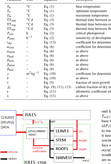
dura-Table 1.Crop model parameters used in JULES-crop.
Parameter Unit Equation Description
Tb ◦C Eq. (1) base temperature
To ◦C Eq. (1) optimum temperature
Tm ◦C Eq. (1) maximum temperature
TTemr ◦C d Eq. (3) thermal time between sowing and emergence
TTveg ◦C d Eq. (3) thermal time between emergence and flowering
TTrep ◦C d Eq. (3) thermal time between flowering and maturity/harvest
Pcrit h Eq. (2) critical photoperiod
Psens h−1 Eq. (2) sensitivity of development rate to photoperiod
rdir – Eq. (13) coefficient for determining relative growth of roots vertically and horizontally
αroot – Eq. (6) coefficient for determining partitioning
αstem – Eq. (6) as above
αleaf – Eq. (6) as above
βroot – Eq. (6) as above
βstem – Eq. (6) as above
βleaf – Eq. (6) as above
γ m2kg−1 Eq. (10) coefficient for determining specific leaf area
δ – Eq. (10) as above
τ – Eq. (5) fraction of stem growth partitioned toCresv
fC – Eqs. (9), (11), (13) carbon fraction of dry matter
κ – Eq. (11) allometric coefficient which relatesCstemtoh
λ – Eq. (11) as above
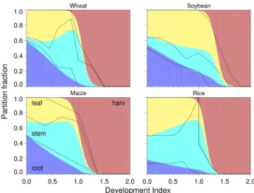
Figure 1.Schematic of JULES-crop.
tion of the cropgrowing seasonare described. Secondly, the equations determining the rate of cropgrowthare described. Lastly, the changes to model structure are outlined. A full listing of new model parameters and variables can be found in Tables 1 and 2, respectively.
2.1 Growing season and development
The crop growing season begins when the crop is sown. This date can either be prescribed (i.e. if it is known) or calcu-lated dynamically based on environmental criteria. In the lat-ter case, sowing only occurs when the soil is wet enough (θ2>θc,2, whereθ2is the soil moisture content in the second
layer andθc,2is the critical soil moisture content in the
sec-ond layer), which is warm enough (Tsoil,3>Tb+2 K, where Tsoil,3is the temperature in the third soil layer andTbis the
base temperature), and when days are not rapidly shortening (dP /dt >−0.02 h d−1, whereP is the day length). We wish
to make users aware of this sowing option; however, we feel it needs further optimising and so results using the dynamic sowing date will not be included here. The use of subsur-face soil moisture and temperature variables prevents sowing occurring too early in response to short-term fluctuations in weather. The rate of day length criterium ensures that crops are not sown too late in the year when conditions for growth are deteriorating.
Once sown, the crop develops through three stages: sow-ing to emergence, emergence to flowersow-ing, and flowersow-ing to maturity. Harvest is assumed to occur at crop maturity. The rate of crop development is related to thermal time. Given the 1.5 m tile temperature (T), an effective temperature (Teff)
is calculated based upon the crop-specific cardinal tempera-tures (Tb, To, Tm– see Table 1 for description).
Teff=
0 for T <Tb
T−Tb for Tb≤T≤To
(To−Tb)
1− T−To
Tm−To
for To<T <Tm
0 for T ≥Tm
. (1)
Teffis greatest and hence development is fastest atT =To.
As temperature falls below or rises aboveTothe rate of
equa-Table 2.Crop model variables in JULES-crop.
Variable Unit Equation Description
New variables
Teff ◦C Eqs. (1), (3) effective temperature
DVI – Eqs. (3), (6), (8), (10) development Index
Cleaf kg C m−2 Eqs. (4), (5), (8), (9) leaf carbon pool
Cstem kg C m−2 Eqs. (4), (5), (11) stem carbon pool
Croot kg C m−2 Eqs. (4), (5), (13) root carbon pool
Charv kg C m−2 Eqs. (5), (7), (8) harvested organ carbon pool
Cresv kg C m−2 Eqs. (5), (7) stem reserve carbon pool
pleaf – Eqs. (5), (6) fraction of NPP partitioned toCleaf
pstem – Eqs. (5), (6), (7) fraction of NPP partitioned toCstem
proot – Eqs. (5), (6) fraction of NPP partitioned toCroot
pharv – Eqs. (5), (6) fraction of NPP partitioned toCharv
P h Eq. (2) photoperiod (day length)
RPE – Eqs. (2), (3) Relative Photoperiod Effect
Existing variables
T ◦C Eq. (1) 1.5 m temperature on each tile
L m2m−1 Eq. (9) leaf area index
SLA m2kg−1 Eqs. (9), (10) Specific Leaf Area
h m Eq. (11) canopy height
5 kg C m−2 Eqs. (4), (5) net primary productivity
Ac kg C m−2 Eq. (4) net carbon assimilation
Rdc kg C m−2 Eq. (4) canopy dark respiration
tion is a “standard” way of calculating effective tempera-ture (Challinor et al., 2004). An important difference to other available models is that JULES-crop simulates a decline of
Teff above the maximum temperature, whereas others keep
Teff at the maximum value no matter how high temperatures get.
For some crops, progress towards flowering is slowed if the day length (P) is less than (greater than) a crop-specific critical photoperiod (Pcrit) for long-day (short-day)
crop types. The degree of sensitivity to the photoperiod is represented by the parameter Psens which is positive for
short-day plants and negative for long-day plants. This con-ceptual approach was motivated by Loomis (1992). There-fore, to slow development Teff is multiplied by the relative
photoperiod effect (RPE), which is defined as follows:
RPE=1−(P−Pcrit)Psens. (2)
The status of crop development is represented by the de-velopment index (DVI) which takes the value of −1 upon sowing, increasing to 0 on emergence, 1 at the end of veg-etative stage and 2 at crop maturity. The rate of increase of DVI is calculated as follows, where TTemris the thermal time
between sowing and emergence, TTveg is the thermal time
between emergence and flowering and TTrepis the thermal
time between flowering and harvest:
dDVI dt =
Teff
TTemr
for −1≤DVI<0 T
eff
TTveg
RPE for 0≤DVI<1
Teff
TTrep
for 1≤DVI<2
. (3)
The growing season ends when DVI=2 at which time the prognostic variables related to crop growth (L, h, Croot, Charv, Cresv) are reset to minimal values close to
0. To prevent growing seasons continuing indefinitely when conditions are no longer suitable, the crop is also harvested if the soil temperature in the second soil layer falls belowTbat
any time after DVI=1 or if LAI>15 (leaf area index). Ver-nalisation, a cold temperature requirement for development in some crops, is not included in this model version. 2.2 Growth
To simulate crop growth, net primary productivity (5) is ac-cumulated over a day and then partitioned between five car-bon pools: root (Croot), structural stem (Cstem), stem reserves
(Cresv), leaves (Cleaf), and harvested organs (Charv). The
estimate respiration loses. Stem carbon is a function of leaf area index (Eq. 42 of Clark et al., 2011) and root carbon is set to equal leaf carbon. Because these carbon pools are now explicitly simulated,5is recalculated for the crop types with the following equation based on an algebraic reduction of the set of equations used in JULES:
5=0.012 1−rg
Ac−Rdc C
root+Cstem Cleaf
, (4)
where rg is the fraction of gross primary productivity less
maintenance respiration that is assigned to growth respira-tion, Ac is the net canopy photosynthesis, and Rdc is the
rate of non-moisture-stressed canopy dark respiration.Cleaf, CstemandCrootare the carbon content of leaf, stem and root,
respectively.
The carbon in 5is accumulated over a day and then di-vided into five crop components according to “partition coef-ficients”, one for each of the four root, stem, leaf and harvest pools defined above and a reserve pool. These components are added to the (state variable) pools of carbon describing the crop.
dCroot
dt =proot5,
dCleaf
dt =pleaf5,
dCstem
dt =pstem5(1−τ ),
dCharv
dt =pharv5,
dCresv
dt =pstem5, τ (5)
whereτ is the fraction of stem carbon that is partitioned in to the reserve pool.proot+pleaf+pstem+pharv=1.0.
Partition coefficients for a given crop are typically prede-fined in process-based crop models according to either the length of time since emergence or to crop development stage (DVI; i.e. a function of thermal time since emergence). They are represented by fixed values for a given period of time (or thermal time) since emergence, and these values are listed in a look-up table and referenced for each iteration of the model (e.g. WOFOST, van Ittersum et al., 2003).
Here we define the partition coefficients as a function of thermal time using six parameters to describe continuously varying partition coefficients over the duration of the crop cycle. We use a multinomial logistic to define this function:
proot=
eαroot+(βrootDVI)
eαroot+(βrootDVI)+eαstem+(βstemDVI)+eαleaf+(βleafDVI)+1,
pstem=
eαstem+(βstemDVI)
eαroot+(βrootDVI)+eαstem+(βstemDVI)+eαleaf+(βleafDVI)+1,
pleaf=
eαleaf+(βleafDVI)
eαroot+(βrootDVI)+eαstem+(βstemDVI)+eαleaf+(βleafDVI)+1,
pharv=
1
eαroot+(βrootDVI)+eαstem+(βstemDVI)+eαleaf+(βleafDVI)+1, (6)
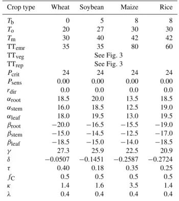
whereαandβ are empirically derived parameters describ-ing the shape of the thermal time-varydescrib-ing partition coeffi-cient for leaves, roots and stems, and DVI is the develop-ment index. Thus, for only six parameters (which is also the absolute minimum number of parameters needed to define partition coefficients for four carbon pools) we can define a much wider range of shapes of thermal time varying partition coefficients. Furthermore, these six parameters can be more feasibly calibrated than a larger number of “look-up” parti-tion coefficients. This parametrisaparti-tion is illustrated in Fig. 2 overlaid with example observed partitioning fractions from de Vries et al. (1989).
Following the formulation of de Vries et al. (1989), once carbon is no longer partitioned to stems, carbon from the stem reserve pool is mobilised to the harvest pool at a rate of 10 % a day:
Charv=Charv+(0.1Cresv) Cresv=0.9Cresv
forpstem<0.01. (7)
Leaf senescence is treated simplistically by mobilising carbon from the leaf to the harvest pool at a rate of 0.05 d−1
once DVI has reached 1.5. This equation was inspired by Eq. (7), but based the period for which senescence starts on a specific DVI value (1.5) rather than waiting for partition-ing of leaves to cease since for some crop types this does not happen.
Charv=Charv+(0.05Cleaf) Cleaf=0.95Cleaf
for DVI>1.5. (8) At the end of each growth time step (24 h), the amount of carbon in the leaves is related to leaf area index (L) by
L=Cleaf
fC
SLA, (9)
where
SLA=γ (DVI+0.06)δ. (10)
Figure 2.Fraction of daily accumulated net primary productivity partitioned to roots (purple), stems (blue), leaves (yellow) and har-vested parts (red) of the crop as a function of development index (DVI; 0=emergence, 1=flowering, 2=maturity) for wheat, rice, soybean and maize.
The amount of carbon in the stem is related to the crop height by (Hunt, 1990)
h=κ C
stem fC
λ
. (11)
The values ofκ andλwere determined by fitting the re-lationship to the paired values of h andCstem at the Mead
FLUXNET site (Verma et al., 2005).
Equations (9) and (11) are rearranged to derive the carbon content of leaves and stems, respectively, before each growth time step.
Because root biomass increases during the crop growing season the fraction of roots in each JULES soil layer varies according to the equation of Arora and Boer (2003) which defines the fraction of roots at depthzas
f =1−e−za, (12)
where
a=dr C
root fC
rdir
, (13)
wheredris 0.5 for all crop types, andrdiris a crop-specific
parameter.
To ensure crop establishment, the growing season is cur-tailed if the sum of root, leaf, stem and reserve carbon falls below the initial seed carbon content (or zero carbon content) if the sowing date is determined dynamically.
2.3 Changes to JULES code structure
The standard version of JULES represents the land surface as a combination of up to nine surface types including five plant
functional types: broadleaf trees, needleleaf trees, C3grass,
C4grass, shrubs, bare soil, inland lakes, snow and ice.
Sur-face fluxes of heat, moisture and momentum are determined independently for each tile before being combined to a single set of fluxes according to the relative fractions of each tile. Each crop type is considered as a different tile. Therefore, it is possible to simulate many crops or crop varieties at a site or grid box in a single integration of JULES, in addition to the standard five plant functional types. The parameters re-quired to represent vegetation within JULES were extended to the crop tile(s). The values were copied across from the JULES default parameters for C3and C4 grass, depending
on the crop photosynthetic capacity (see Table 3).
The values of the parameters required in Eqs. (1)–(13) de-termine which crops are being simulated and can be varied according to different user requirements, e.g. crop species (e.g. maize or wheat), generic crop type (e.g. C3cereals) or
cultivar (e.g. soybean PS123121 or soybean 21h321). Each parameter is described in Table 1. Values for each parameter can be determined by calibration against relevant observa-tional data such as leaf area index, biomass, and yield from agricultural field stations. For this study such an exercise was not performed. Instead, suitable values were determined from either the literature or by tuning to fit site-level data in order to establish a model version that could be evaluated at site and global scales.
3 Global simulation 3.1 Model set-up
To evaluate the potential of JULES-crop as a global gridded crop model, simulations for the period 1960–2010 were per-formed over the global domain. Four crop types were simu-lated: wheat, soybean, maize and rice. Parameter values are in Table 4 and were either taken from the crop science litera-ture or calibrated as described below. Specifically, the values for the partition parametersαroot, stem, leaf andβroot, stem, leaf
and the specific leaf area coefficientsγandδwere calibrated against data in de Vries et al. (1989). The allometric coeffi-cientsκ andλwere determined by calibration against paired crop height and stem biomass data from FLUXNET sites. The cardinal temperatures (Tb,To, and Tm) were specified values in line with the range of values reported in the litera-ture (see Porter and Gawith, 1999, and Sanchez et al., 2014). The effect of photoperiod was not included (by settingPcritto
24) due to our method of determining thermal time between emerging and flowering (TTveg) and thermal time between
flowering and harvest (TTrep) (see below).
The parameterrdirwas set to 0 for all crop types, which
lead-Table 3.JULES plant functional type parameters extended to represent crop types wheat, soybean, maize and rice.
Crop type Wheat Soybean Maize Rice
c3 1 1 0 1
dr 0.5 0.5 0.5 0.5
dqcrit 0.1 0.1 0.075 0.1
fd 0.015 0.015 0.025 0.015
f0 0.9 0.9 0.8 0.9
neff 8.00×10⁻⁴ 8.00×10⁻⁴ 4.00×10⁻⁴ 8.00×10⁻⁴
nl(0) 0.073 0.073 0.06 0.073
σl 0.032 0.032 0.025 0.032
Tlow 0 0 13 0
Tupp 36 36 45 36
Table 4.Parameter values used to represent crop types wheat, soy-bean, maize and rice. See Table 1 for parameter definitions.
Crop type Wheat Soybean Maize Rice
Tb 0 5 8 8
To 20 27 30 30
Tm 30 40 42 42
TTemr 35 35 80 60
TTveg See Fig. 3
TTrep See Fig. 3
Pcrit 24 24 24 24
Psens 0.00 0.00 0.00 0.00
rdir 0.0 0.0 0.0 0.0
αroot 18.5 20.0 13.5 18.5
αstem 16.0 18.5 12.5 19.0
αleaf 18.0 19.5 13.0 19.5
βroot −20.0 −16.5 −15.5 −19.0
βstem −15.0 −14.5 −12.5 −17.0
βleaf −18.5 −15.0 −14.0 −18.5
γ 27.3 25.9 22.5 20.9
δ −0.0507 −0.1451 −0.2587 −0.2724
τ 0.40 0.18 0.35 0.25
fC 0.5 0.5 0.5 0.5
κ 1.4 1.6 3.5 1.4
λ 0.4 0.4 0.4 0.4
ing to poor crop growth. Therefore, the effect was “turned off”. The parametrisation was left in the model to allow other model users to experiment further with dynamic root growth. The global model runs were driven by the CRU-NCEP v4 climate data extended to include 2012 (N. Viovy, personal communication, 2013) as used by the Global Carbon Project (Le Quéré et al., 2013). This was regridded to a N96 grid (1.875◦
longitude×1.25◦
latitude) and used with ancillaries from HadGEM2-ES (Collins et al., 2011; Jones et al., 2011) to evaluate the performance of the model in a Earth system model set-up. A multi-layer canopy radiation scheme was used, accounting for direct/diffuse radiation components in-cluding sunflecks (can_ran_mod=5). The main run was from 1960 to 2010 and the spin-up consisted of repeating
the first 10 years 5 times. The sowing dates were taken from Sacks et al. (2010), and a value for each land grid box was obtained using nearest-neighbour extrapolation. The values of TTvegand TTrepwere allowed to vary spatially and
deter-mined such that, when used with the CRU-NCEP tempera-ture climatology 1990–2000 and the Sacks et al. (2010) sow-ing date, the crop reached DVI=2.0 at the Sacks et al. (2010) harvesting dates, withx=(TTTTveg
veg+TTrep) =0.5,0.45,0.6,0.6 for soybean, maize, wheat, and rice, respectively. Photope-riod sensitivity was not considered.This is because including it would have made calculating TTvegand TTrepalmost
im-possible, because three variables would need calibrating at each grid cell (total TT, critical photoperiod, and sensitivity to photoperiod) from one observation (growing season du-ration). For comparison a control run was completed using the same model set-up but with the crop code switched off. This run is used to assess performance against the standard land surface scheme in the Met Office Hadley Centre Earth System Model – HadGEM2-ES.
Figure 3 shows the planting date of Sacks et al. (2010) and the derived maps of TTvegand TTrep. Sacks et al. (2010)
Figure 3.Global distribution planting date from Sacks et al. (2010), interpolated to NCEP grid, and the thermal time from emergence to flowering (TT_veg) and from flowering to harvest (TT_rep) for each crop type. See text for details of calculation.
study) to the annual accumulated thermal time and then used that relationship to determine thermal time requirements un-der future climate. The approach in this study was chosen as the simplest and most likely to achieve growing seasons of lengths close to observed. Due to the absence of a vernali-sation parametrivernali-sation in the model only spring wheat was considered. The crop fractions were taken from Monfreda et al. (2008) and regridded to the N96 HadGEM2-ES resolu-tion. Monfreda et al. (2008) provide observations in the year 2000 which were used to describe the crop coverages for the whole integration period due to a lack of available data sets covering this time period.
3.2 Evaluation
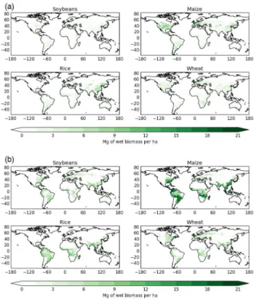
The simulated grid box annual yield for each crop averaged over the 50 years is shown in Fig. 4 alongside global gridded observations for circa 2000 (Monfreda et al., 2008). Figure 4 shows that in general the model is underestimating yields in arid, irrigated regions and overestimating them in tropical re-gions. In particular, simulated maize yields are significantly larger than observations in tropical regions. Given that the model does not include any information on the yield gap (the difference between actual farm-level yield and potential yield) or important land management such as irrigation the spatial variability of model output should not be too closely compared to that of observed yield. Instead, a greater appre-ciation of model performance can be gained from examining the year to year fluctuations in yield, given that the effects of changes in management and technology materialise over several years.
Figures 5 and 6 show the simulated global- and country-level yields for wheat, soybean, maize and rice between 1960
Figure 4.Global distribution of average wheat, soybean, maize and rice yield (Mg ha−1) in(a)observations (Monfreda et al., 2008)
regridded to N96 resolution and(b)JULES-crop global simulations (assuming a moisture content of 16 % and a carbon fraction of 0.5).
Figure 6.Simulated (red), observed (black dashed) and detrended observed (black) country-level yields of(a)maize,(b)soybean,(c)rice and(d)wheat between 1961 and 2008. Values in the top right are results of a correlation between detrended observations and JULES-crop simulations.
and 2008 compared to the reported yields of FAO (2014). Simulated global yield was determined by multiplying the simulated annual maximum yield at each grid cell by the ob-served harvested area from Monfreda et al. (2008) regridded to the HadGEM2-ES spatial resolution. This grid cell esti-mate of production was summed over all grid cells to produce an estimate of global production which was then divided by the total harvested area to provide an estimate of global yield. Grid cell yields were determined from the annual maximum value of Charv which was multiplied by 2 to convert from carbon mass to total biomass, by 1.16 to account for grain moisture content, and by 10 to convert from kilograms per squared metre to megagrams per hectare. Not all grid cells were included in the analysis. Cells were excluded if the an-nual maximum DVI was less than 1.5 which was possible if the growing season was curtailed if LAI>15 ortsoil,2<Tbse.
A similar analysis was conducted to determine country-level
yields with averages taken over all grid cells within a partic-ular country. Country yield observations were de-trended for comparison with model output. This is because the increas-ing trend in yield observations over the last 50 years is due to improvements in agricultural technology and management and increasing atmospheric carbon dioxide. This trend is not reproduced by the model as these processes were not repre-sented in our set-up.
Figure 7.Country crop area weighted annual cycle of crop type (top) and grid-box mean (middle) leaf area index (LAI) and grid-box mean (bottom) net primary production (NPP). Area averages weighted by crop area in top panel, and total plant functional type area in middle and bottom panels. Vertical bars indicate standard deviation of monthly values.
countries such as the USA (r=0.39) and India (r=0.52) JULES-crop is able to reasonably capture inter-annual vari-ability of yields (Fig. 6b). For rice, yield levels are higher than reported, variability is overestimated and not correlated with observations (r=0.24). At the country level, model simulations in India (r=0.57) correlate with observations (Fig. 6c). The average simulated yield level for wheat is sim-ilar to the most recent observations; however, when com-paring the year to year fluctuations in yield, the correlation between simulated and observed yields is low (r=0.019). Because JULES-crop only simulates spring wheat then the comparison to reported wheat yields is slightly unfair given that the majority of wheat produced globally is from winter varieties. It is encouraging that the best agreement between simulated and observed yield fluctuations at the national level is for Turkey (r=0.46) and Australia (r=0.53), in which spring wheat varieties dominate.
For all crops there is a tendency for JULES-crop to simu-late larger variability than observed. This may in part be ex-plained by the lack of certain processes in the model (partic-ularly those to do with land management). For example, not including a representation of irrigation in the model may ex-plain why the model predicts lower yields than observations as irrigation would act to reduce the extent of crop failure in drought years. The model also does not include the impacts of pests and disease which may reduce overall yields in some
years. Importantly, the model does not as yet include a ni-trogen cycle which may reduce overall GPP (gross primary production), bringing the simulations in line with observa-tions. This may also explain why there are strong deviations between the magnitude of observed and modelled yield in tropical countries where climatic conditions for growth are good in the absence of the limitations described above.
For some countries simulations of yield capture the mag-nitude and variability of observations. In other countries the model reproduces the variability in yield but over-predicts the magnitude. There are also countries where the model per-forms poorly in simulating both variability and magnitude. This variety of results is due in part to the use of generic parametrizations for global model runs which is a limitation of this type of Earth system model set-up. By using parame-ters that do not vary spatially we can not fully represent the range of crop varieties that are found globally.
Figure 8. Country crop area weighted average mean annual cycle of surface moisture flux (E), sensible heat flux (H), net short-wave radiation (SWnet) and upward long-wave radiation (LWup) from JULES-crop simulation (red) and standard JULES simulation (black) forced
with CRU-NCEP meteorological driving data. Vertical bars indicate standard deviation of monthly values.
LAI values are shown in Fig. 7 for four major crop producing countries. To produce the country averages, grid cell LAI are combined by weighting by the grid cell contribution to total country crop area. In the USA and China each crop growing season occupies the similar set of summer months, whereas for India and Brazil the wheat cropping season is distinct from the other three crops. Peak LAI is greatest in Brazil and lowest in China, which is most likely a reflection of the ab-sence of irrigation in the model and the relative abundance of rainfall in each country. In comparison to the standard JULES configuration the addition of crops adds a season-ality to LAI as there is no default seasonseason-ality to vegetation characteristics in JULES. The annual variation of crop LAI is dampened when aggregated with the other plant functional types, which explains the non-zero LAI in the non-growing season in the JULES-crop simulation. Figure 7 shows that the inclusion of crops alters the grid box net primary produc-tion (NPP) in terms of the timing of peak fluxes. There are also lower fluxes in winter due to the more realistic treatment of LAI at this time. Therefore, including a representation of crops in JULES may help improve the seasonality of LAI, which affects carbon fluxes.
Figure 8 shows that the impact of these differences in veg-etation size during the year is greatest for the surface mois-ture flux and sensible heat flux rather than the components of the radiation balance. The largest impacts are on the sen-sible heat flux towards the end of the crop growing season
which is higher with the inclusion of crops. For India, there is a concomitant decrease in the surface moisture flux, imply-ing that the total available energy at the surface is unaltered but is partitioned differently between sensible and latent heat fluxes. The impact of JULES-crop on the energy balance is however minimal. In this configuration the model is forced by prescribed meteorology at screen height. This has the ten-dency to dampen the model in comparison to a full atmo-spheric simulation in which the boundary layer state is able to evolve. It may, therefore, be expected that a GCM (global climate model) may be more sensitive to changes in the sur-face state.
4 Site simulation 4.1 Model set-up
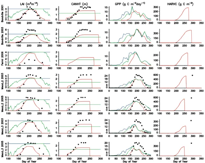
Figure 9.Simulated (solid lines) and observed (dots) leaf area index (LAI), canopy height (CANHT), gross primary production (GPP) and harvest carbon (HARVC) at a range of FLUXNET sites and years. Simulations performed with JULES-crop crop type soybean (red), standard JULES C3grass plant functional type with phenology (green), and standard JULES C3grass plant functional type without phenology (blue).
JULES-crop parametrisation. For the JULES-crop simula-tion, the fractional coverage of the relevant crop type was set to 1 with all other functional types set to 0. For the JULES (non-crop) simulations, the fractional coverage of the rele-vant grass functional type (i.e. C3grass for soybean, C4for
maize) was set to 1. All crop parameters were prescribed the same value as in the global simulations. The sowing date and thermal time requirements were taken from the relevant grid cell for each site.
4.2 Evaluation
Figures 9 and 10 compare JULES-crop simulations for the soybean crop type with standard JULES C3grass plant
func-tional type with and without phenology, and with observa-tions where available. The crop parametrisation captures the evolution of LAI and canopy height across the season, al-though the model underestimates these growth variables. The model also simulates lower GPP fluxes compared to obser-vations; however, crop yields are comparable. The standard C3grass with phenology configuration of JULES also
simu-lates growth and decay of vegetation cover but over a longer period of time than the observed growing season. Without the phenology routine the LAI is set to the default for C3
grass of 2.0 all year. Interestingly, the more realistic lation of vegetation cover does not lead to improved simu-lation of surface fluxes. At all sites similar characteristics of the simulations are evident. During winter all three configu-rations simulate similar latent and sensible heat fluxes in line with observations (Fig. 10). Towards the start of the grow-ing season the standard configuration of JULES with con-stant LAI=2.0 overestimates latent heat flux due to an un-realistically large vegetation coverage. The simulations with phenology and crops have lower vegetation cover and simu-late lower simu-latent heat flux but are still noticeably greater than observations. At around the peak of crop cover, all simula-tions underestimate the latent heat flux and overestimate the sensible heat flux due to lower simulated LAI compared to observations.
Figure 10.Simulated (solid lines) and observed (dots) latent (LE) and sensible (H) heat fluxes at a range of FLUXNET sites and years. Simulations performed with JULES-crop crop type soybean (red), standard JULES C3grass plant functional type with phenology (green),
and standard JULES C3grass plant functional type without phenology (blue).
at all evaluation sites. Similarly, GPP and yields are lower than observed although the seasonal pattern of GPP is close to observations. Overall, model simulations broadly capture the patterns of latent and sensible heat fluxes although, again, there are no major improvements in model performance with the explicit inclusion of crops. At Fermi, in 2006, the crop-specific simulation captures the observed evolution of LAI reasonably well with peak LAI slightly closer to observations than the standard JULES simulations. However, this, again, does not improve the simulation of heat fluxes.
All model configurations overestimate the partitioning of energy in to latent heat before the growing season begins and underestimate it during the crop growing season, despite widely varying LAI values. This could be due to the rela-tively weak LAI-surface conductance relationship found in JULES (Lawrence and Slingo, 2004). This is reflected in the low sensitivity to LAI between fixed phenology and seasonal phenology. In these simulations we would therefore not ex-pect a large response to an alternative representation of crop LAI phenology. This comparison serves as a reminder that improving the realism of a model may not guarantee
im-proved performance in the model in other aspects. The re-sults also show that JULES (crop and standard configura-tions) is not able to capture the magnitude of observed GPP fluxes. This suggests that using the standard physiological parameters for C3 and C4 grasses is not appropriate when
representing crops particularly as JULES does not include nitrogen fertilisation explicitly. Tuning of parameters that de-scribe leaf nitrogen, for example, may improve fluxes of GPP and hence overall yields. It is also worth noting that the pa-rameters used for the crop model in the site simulations are from the global set-up and hence probably not optimal for site simulations.
5 Discussion and conclusions
num-Figure 11.Simulated (solid lines) and observed (dots) LAI, CANHT, GPP and HARVC at a range of FLUXNET sites and years. Simulations
performed with JULES-crop crop type maize (red), standard JULES C3grass plant functional type with phenology (green), and standard
JULES C3grass plant functional type without phenology (blue).
ber of crop cultivars of the same crop type at the site scale forced with weather observations and (c) to assess how crops may impact on biogeophysical feedbacks to climate includ-ing albedo, partitioninclud-ing of turbulent fluxes and seasonality of LAI. In this paper we present results from a generic, crop functional type parametrisation implemented at both global and site scales to show how this model performs in an Earth system model context. Having the aim of generality neces-sarily means that the model loses out in terms of specificity. However, with further effort it should be possible to tailor the model set-up for more specific applications but with the re-quirement that attention is given to the choice of parameter values. Default values are provided here as a starting point for model development and initial evaluation.
These results demonstrate the importance of evaluating the performance of JULES-crop in a holistic sense, assess-ing both its ability to simulate land surface fluxes in addi-tion to crop growth and development dynamics and to recog-nise that identified biases in performance are the result of the combined JULES-crop model, not just the added crop component. Adding a crop parametrisation has increased the
complexity of JULES. However, this has not led to an im-mediate improvement in the model’s simulation of surface fluxes, at least at the measurement sites examined. More ef-fort needs to go into developing the parameter sets for crops within JULES, particularly for the existing set of plant func-tional type parameters which control productivity.
How-Figure 12.Simulated (solid lines) and observed (dots) LE and H fluxes at a range of FLUXNET sites and years. Simulations performed with JULES-crop crop type maize (red), standard JULES C3grass plant functional type with phenology (green), and standard JULES C3grass
plant functional type without phenology (blue).
ever, we have deliberately not introduced a yield gap adjust-ment as it would not be physically based and as such would be difficult to apply to future simulations. It is, however, im-portant to capture regional differences due to management as they will effect patterns in productivity and hence feed-backs to the climate. In an Earth system model context it is better to represent these management processes explicitly where possible, as they effect not only crop growth but also may well influence the local climate directly (e.g. irrigation; Sacks et al., 2009).
As a yield simulation model, there are encouraging signs that JULES-crop can simulate variability in yield associated with climate fluctuations. However, it is clear that JULES-crop overestimates the magnitude of this variability. Whilst the absence of irrigation is most likely a contributing factor to the overestimation of yield variability, the implication that the model is too sensitive to changes in environmental con-ditions should also be investigated further.
Including crops in JULES gives a more realistic seasonal cycle of leaf area index, which affects the seasonality of car-bon fluxes (timing of peak flux and lower winter fluxes). This
was seen at both the global and site levels. The impact of crops on the energy balance was to alter the partitioning of latent and sensible heat fluxes particularly in winter, which led to small impacts on temperature in some countries. These impacts were marginal at the country and site scales despite quite large differences in LAI. It is possible that the rela-tionship between LAI and evaporation is too weak in JULES (Lawrence and Slingo, 2004), which may explain why a more realistic representation of LAI did not improve the energy fluxes. We may expect a higher sensitivity in fully coupled atmosphere models.
for example the application of fertiliser to increase leaf nitro-gen contents impacting on photosynthesis. For applications of JULES-crop that rely on accurate yield simulations, the inclusion of either a yield gap variable or the factors that determine it such as fertiliser applications, pest control, and soil fertility should be a priority for future model develop-ment. Inclusion of winter wheat is also of high priority for JULES-crop. This is important for use of JULES-crop as a yield simulation model but also an Earth system model, as the additional presence of vegetation cover from autumn to spring would impact on surface characteristics (albedo, heat capacity, etc.).
Acknowledgements. This work was supported by the Joint
DECC/Defra Met Office Hadley Centre Climate Programme and the National Centre for Atmospheric Science. Richard Betts was also supported by the University of Exeter and the EU High-End cLimate Impacts and eXtremes (HELIX) project.
Edited by: G. Folberth
References
Arora, V. and Boer, G.: A representation of variable root distribution in dynamic vegetation models, Earth Interact., 7, 1–19, 2003. Asseng, S., Ewert, F., Rosenzweig, C., Jones, J. W., Hatfield, J. L.,
Ruane, A. C., Boote, K. J., Thorburn, P. J., Rötter, R. P., Cam-marano, D., Brisson, N., Basso, B., Martre, P., Aggarwal, P. K., Angulo, C., Bertuzzi, P., Biernath, C., Challinor, A. J., Doltra, J., Gayler, S., Goldberg, R., Grant, R., Heng, L., Hooker, J., Hunt, L. A., Ingwersen, J., Izaurralde, R. C., Kersebaum, K. C., Müller, C., Kumar, S. N., Nendel, C., O’Leary, G., Olesen, J. E., Os-borne, T. M., Palosuo, T., Priesack, E., Ripoche, D., Semenov, M. A., Shcherbak, I., Stedutoand, P., Stöckle, C., Stratonovitch, P., Streck, T., Supit, I., Tao, F., Travasso, M., Waha, K., Wal-lach, D., White, J. W., Williams, J. R., and Wolf, J.: Uncertainty in simulating wheat yields under climate change, Nature Clim. Change, 3, 827–832, 2013.
Best, M. J., Pryor, M., Clark, D. B., Rooney, G. G., Essery, R. L. H., Ménard, C. B., Edwards, J. M., Hendry, M. A., Porson, A., Gedney, N., Mercado, L. M., Sitch, S., Blyth, E., Boucher, O., Cox, P. M., Grimmond, C. S. B., and Harding, R. J.: The Joint UK Land Environment Simulator (JULES), model description – Part 1: Energy and water fluxes, Geosci. Model Dev., 4, 677–699, doi:10.5194/gmd-4-677-2011, 2011.
Betts, R. A., Golding, N., Gonzalez, P., Gornall, J., Kahana, R., Kay, G., Mitchell, L., and Wiltshire, A.: Climate and land use change impacts on global terrestrial ecosystems and river flows in the HadGEM2-ES Earth system model using the represen-tative concentration pathways, Biogeosciences, 12, 1317–1338, doi:10.5194/bg-12-1317-2015, 2015.
Bondeau, A., Smith, P., Zaehle, S., Schaphoff, S., Lucht, W., Cramer, W., Gerten, D., Lotze-Campen, H., Müller, C., Reich-stein, M., and Smith, B.: Modelling the role of agriculture for the 20th century global terrestrial carbon balance, Glob. Change Biol., 13, 679–706, 2007.
Challinor, A., Wheeler, T., Craufurd, P., Slingo, J., and Grimes, D.: Design and optimisation of a large-area process-based model for annual crops, Agr. Forest Meteorol., 124, 99–120, doi:10.1016/j.agrformet.2004.01.002, 2004.
Chen, F. and Xie, Z.: Effects of crop growth and development on regional climate: a case study over East Asian monsoon area, Clim. Dynam., 38, 2291–2305, 2012.
Clark, D. B., Mercado, L. M., Sitch, S., Jones, C. D., Gedney, N., Best, M. J., Pryor, M., Rooney, G. G., Essery, R. L. H., Blyth, E., Boucher, O., Harding, R. J., and Cox, P. M.: The Joint UK Land Environment Simulator (JULES), Model description –Part 2: Carbon fluxes and vegetation, Geosci. Model Dev. Discuss., 4, 641–688, doi:10.5194/gmdd-4-641-2011, 2011.
Collins, W. J., Bellouin, N., Doutriaux-Boucher, M., Gedney, N., Halloran, P., Hinton, T., Hughes, J., Jones, C. D., Joshi, M., Lid-dicoat, S., Martin, G., O’Connor, F., Rae, J., Senior, C., Sitch, S., Totterdell, I., Wiltshire, A., and Woodward, S.: Development and evaluation of an Earth-system model – HadGEM2, Geosci. Model Dev. Discuss., 4, 997–1062, doi:10.5194/gmdd-4-997-2011, 2011.
de Vries, F. P., Jansen, D., ten Berge, H., and Bakema, A.: Simu-lation of ecophysiological processes of growth in several annual crops, p. 271, Pudoc Wageningen, 1989.
Deryng, D., Sacks, W. J., Barford, C. C., and Ramankutty, N.: Sim-ulating the effects of climate and agricultural management prac-tices on global crop yield, Global Biogeochem. Cy., 25, GB2006, doi:10.1029/2009GB003765, 2011.
FAO: FAOSTAT, http://faostat.fao.org/site/291/default.aspx, last ac-cess: June 2014.
Hunt, R.: Basic Growth Analysis: plant growth analysis for begin-ners, Cambridge University Press, UK, 1990.
Jones, C. D., Hughes, J. K., Bellouin, N., Hardiman, S. C., Jones, G. S., Knight, J., Liddicoat, S., O’Connor, F. M., Andres, R. J., Bell, C., Boo, K.-O., Bozzo, A., Butchart, N., Cadule, P., Corbin, K. D., Doutriaux-Boucher, M., Friedlingstein, P., Gor-nall, J., Gray, L., Halloran, P. R., Hurtt, G., Ingram, W. J., Lamar-que, J.-F., Law, R. M., Meinshausen, M., Osprey, S., Palin, E. J., Parsons Chini, L., Raddatz, T., Sanderson, M. G., Sellar, A. A., Schurer, A., Valdes, P., Wood, N., Woodward, S., Yoshioka, M., and Zerroukat, M.: The HadGEM2-ES implementation of CMIP5 centennial simulations, Geosci. Model Dev., 4, 543–570, doi:10.5194/gmd-4-543-2011, 2011.
Kucharik, C. and Brye, K.: Integrated BIosphere Simulator (IBIS) yield and nitrate loss predictions for Wisconsin maize receiving varied amounts of nitrogen fertilizer, J. Environ. Qual., 32, 247– 268, 2003.
Lawrence, D. and Slingo, J.: An annual cycle of vegetation in a GCM. Part I: implementation and impact on evaporation, Clim. Dynam., 22, 87–105, doi:10.1007/s00382-003-0366-9, 2004. Le Quéré, C., Peters, G. P., Andres, R. J., Andrew, R. M., Boden,
Wan-ninkhof, R., Wiltshire, A., and Zaehle, S.: Global carbon budget 2013, Earth Syst. Sci. Data, 6, 235–263, doi:10.5194/essd-6-235-2014, 2014.
Levis, S.: Modeling vegetation and land use in models of the Earth System, Climate Change, 1, 840–856, 2010.
Levis, S., Bonan, G., Kluzek, E., Thornton, P. E., Jones, A., Sacks, W. J., and Kucharik, C. J.: Interactive cop management in the Community Earth System Model (CESM1): Seasonal influences on land-atmoshpere fluxes, J. Climate, 25, 4839–4859, 2012. Licker, R., Johnston, M., Foley, J., Barford, C., Kucharik, C.,
Mon-freda, C., and Ramankutty, N.: Mind the gap: how do climate and agricultural management explain the yield gap of crop-lands around the world, Global Ecol. Biogeogr., 19, 769–782, doi:10.1111/j.1466-8238.2010.00563.x, 2010.
Lokupitiya, E., Denning, S., Paustian, K., Baker, I., Schaefer, K., Verma, S., Meyers, T., Bernacchi, C. J., Suyker, A., and Fischer, M.: Incorporation of crop phenology in Simple Biosphere Model (SiBcrop) to improve land-atmosphere carbon exchanges from croplands, Biogeosciences, 6, 969–986, doi:10.5194/bg-6-969-2009, 2009.
Loomis, R. S. and Connor, D.: Crop Ecology: productivity and man-agement in agricultural systems, Cambridge University Press, UK, 1992.
McPherson, R., Stensrud, D., and Crawford, K. C.: The impact of Oklahoma’s winter wheat belt on the mesoscale environment, Mon. Weather Rev., 132, 405–421, 2004.
Monfreda, C., Ramankutyy, N., and Foley, J.: Farming the planet: 2. Geogrpahic distribution of cropa areas, yields, physiological types, anmd net primary production in the year 2000, Global Bio-geochem. Cy., 22, GB1022, doi:10.1029/2007GB002947, 2008. Osborne, T., Lawrence, D., Challinor, A., Slingo, J., and Wheeler, T.: Development and assessment of a coupled crop-climate model, Glob. Change Biol., 13, 169–183, 2007.
Osborne, T., Rose, G., and Wheeler, T.: Variation in the global-scale impacts of climate change on crop productivity due to climate model uncertainty and adaptation, Agr. Forest Meteorol., 170, 183–194, doi:10.1016/j.agrformet.2012.07.006, 2013.
Porter, J. and Gawith, M.: Temperatures and the growth and development of wheat: a review, Eur. J. Agron., 10, 23–36, doi:10.1016/S1161-0301(98)00047-1, 1999.
Sacks, W., Cook, B., Buenning, N., Levis, S., and Helkowski, J.: Ef-fects of global irrigation on the near-surface climate, Clim. Dy-nam., 33, 159–175, doi:10.1007/s00382-008-0445-z, 2009. Sacks, W. J., Deryng, D., Foley, J. A., and Ramankutty, N.: Crop
planting dates: an analysis of global patterns, Global Ecol. Biogeogr., 19, 607–620, doi:10.1111/j.1466-8238.2010.00551.x, 2010.
Sanchez, B., Rasmussen, A., and Porter, J.: Temperatures and the growth and development of maize and rice: a review, Glob. Change Biol., 20, 408–417, doi:10.1111/gcb.12389, 2014. Thornton, P. E., Doney, S. C., Lindsay, K., Moore, J. K.,
Ma-howald, N., Randerson, J. T., Fung, I., Lamarque, J.-F., Fed-dema, J. J., and Lee, Y.-H.: Carbon-nitrogen interactions regu-late climate-carbon cycle feedbacks: results from an atmosphere-ocean general circulation model, Biogeosciences, 6, 2099–2120, doi:10.5194/bg-6-2099-2009, 2009.
Van den Hoof, C., Hanert, E., and Vidale, P.-L.: Simulating dy-namic crop growth with an adapted land surface model JULES-SUCROS: Model development and validation, Agr. Forest Mete-orol., 151, 137–153, 2011.
van Ittersum, M., Leffelaar, P., van Keulen, H., Kropff, M., Bas-tiaans, L., and Goudriaan, J.: On approaches and applications of the Wageningen crop models, Eur. J. Agron., 18, 201–234, doi:10.1016/S1161-0301(02)00106-5, 2003.