www.the-cryosphere.net/5/773/2011/ doi:10.5194/tc-5-773-2011
© Author(s) 2011. CC Attribution 3.0 License.
The Cryosphere
Simulation of permafrost and seasonal thaw depth
in the JULES land surface scheme
R. Dankers1, E. J. Burke1, and J. Price1,*
1Met Office Hadley Centre, Exeter, UK
*now at: College of Life and Environmental Sciences, University of Exeter, Exeter, UK
Received: 1 April 2011 – Published in The Cryosphere Discuss.: 26 April 2011
Revised: 6 September 2011 – Accepted: 7 September 2011 – Published: 27 September 2011
Abstract. Land surface models (LSMs) need to be able to simulate realistically the dynamics of permafrost and frozen ground. In this paper we evaluate the performance of the LSM JULES (Joint UK Land Environment Simula-tor), the stand-alone version of the land surface scheme used in Hadley Centre climate models, in simulating the large-scale distribution of surface permafrost. In particular we look at how well the model is able to simulate the seasonal thaw depth or active layer thickness (ALT). We performed a number of experiments driven by observation-based climate datasets. Visually there is a very good agreement between areas with permafrost in JULES and known permafrost dis-tribution in the Northern Hemisphere, and the model captures 97 % of the area where the spatial coverage of the permafrost is at least 50 %. However, the model overestimates the total extent as it also simulates permafrost where it occurs spo-radically or only in isolated patches. Consistent with this we find a cold bias in the simulated soil temperatures, especially in winter. However, when compared with observations on end-of-season thaw depth from around the Arctic, the ALT in JULES is generally too deep. Additional runs at three sites in Alaska demonstrate how uncertainties in the precipitation input affect the simulation of soil temperatures by affecting the thickness of the snowpack and therefore the thermal insu-lation in winter. In addition, changes in soil moisture content influence the thermodynamics of soil layers close to freez-ing. We also present results from three experiments in which the standard model setup was modified to improve physical realism of the simulations in permafrost regions. Extending the soil column to a depth of 60 m and adjusting the soil pa-rameters for organic content had relatively little effect on the
Correspondence to:R. Dankers ([email protected])
simulation of permafrost and ALT. A higher vertical resolu-tion improves the simularesolu-tion of ALT, although a consider-able bias still remains. Future model development in JULES should focus on a dynamic coupling of soil organic carbon content and soil thermal and hydraulic properties, as well as allowing for sub-grid variability in soil types.
1 Introduction
The impact of climate change on permafrost in the cir-cumpolar arctic has received much attention in recent years (Anisimov and Nelson, 1996; Stendel and Christensen, 2002; Lawrence and Slater, 2005; Lawrence et al., 2008; Zhang et al., 2008). This is partly because of the dramatic rise in tem-perature at northern high latitudes that is projected by many General Circulation Models (GCMs) for the coming cen-turies (Kattsov et al., 2005; Christensen et al., 2007). Addi-tionally, there has been a growing concern about the amount of organic matter stored in currently frozen soils that may start to decompose once the permafrost thaws (Zimov et al., 2006; Schuur et al., 2008). Depending on whether this de-composition takes place under aerobic or anaerobic condi-tions, it may result in enhanced emissions of carbon diox-ide (CO2) or methane (CH4) and other greenhouse gases,
Recent years have seen a growing number of permafrost models, often developed with a specific application in mind (Riseborough et al., 2008). Conventional permafrost mod-elling often assumes the soil thermal regime is in equilib-rium with the climate. In reality the thermal state of the ground depends on a number of complex interactions be-tween soil, vegetation, snow and hydrology (Sturm et al., 2001; Smith et al., 2005). When applied over large regions, permafrost modelling is further complicated by the complex patterns of vegetation and topography typical for arctic envi-ronments (Sazonova and Romanovsky, 2003; Stendel et al., 2007) and limited data availability on meteorological condi-tions, as well as soil and land surface properties. Anisimov et al. (2002) and Anisimov (2009) addressed part of this prob-lem by using a stochastic modelling approach to account for the high spatial variability in large-scale permafrost models. Aside from portraying the level of uncertainty in the input parameters, the output from such a model can be used to es-timate the probability of permafrost temperature and thaw depth exceeding a given threshold at a certain location.
In weather and climate models, the interaction between the atmosphere and the land surface is simulated by land sur-face models (LSMs). These LSMs are designed to repre-sent the physical processes controlling the exchange of heat and moisture in order to solve the surface energy balance, typically by partitioning the available energy between evap-orative, sensible and ground heat fluxes. In climate science there has been a growing recognition that different parts of the Earth system affect one another and that these feedbacks, which often involve land ecosystem-atmosphere interactions, need to be included in the models in order to achieve im-proved projections for the future. Consequently, LSMs have grown in complexity in an effort to include processes such as changes in vegetation cover, carbon cycling in terrestrial ecosystems and the direct effect of rising CO2concentrations
on plant physiology. In spite of their limitations (see e.g. Slater et al., 2001; Nijssen et al., 2003), LSMs offer the op-portunity to study changes in the terrestrial environment in an integrated and consistent way and to explore key interactions between the different impacts (Betts, 2007). LSMs are thus not specific permafrost models, but if claims of LSMs be-ing physically process-based models have any validity, they ought to be capable of simulating the dynamics of permafrost and frozen ground with some realism.
The aim of this paper is to evaluate the performance of the Joint UK Land Environment Simulator (JULES) (Blyth et al., 2006), the LSM used within the Hadley Centre climate models, in simulating large-scale features of surface per-mafrost, and to identify areas for improvement. To achieve this we performed a number of off-line experiments with JULES driven by observation-based climate datasets. We also present results from two experiments in which the stan-dard model setup was modified with the aim of improving the physical realism of the simulations in permafrost regions.
2 JULES model description
JULES is the stand-alone version of the land surface scheme used in the Hadley Centre climate models (Blyth et al., 2006). It is based on the Met Office Surface Exchange Scheme (MOSES) described by Cox et al. (1999) and Essery et al. (2001) and combines a complex energy and water bal-ance model with a dynamic vegetation model. As a commu-nity model JULES is available for everybody to use and/or to contribute to its further development (see the JULES website http://www.jchmr.org/jules for more details).
JULES describes the physical, biophysical and biochem-ical processes that control the exchange of radiation, heat, water and carbon between the land surface and the atmo-sphere. It can be applied as a point or a grid model. When applied in distributed mode each grid box can have several sub-grid land cover fractions or “tiles”. JULES has five vegetation tiles representing different plant functional types (broad-leaf trees, needle-leaf trees, C3 (temperate) grass, C4 (tropical) grass, and shrubs) and four non-vegetated surface tiles (urban, inland water, bare soil and ice). Each tile has its own surface temperature, shortwave and longwave radia-tive fluxes, sensible and latent heat fluxes, ground heat flux, canopy moisture content, snow mass and snow melt. The soil underneath the land cover tiles is, however, assumed to be homogeneous across the grid box. By default, JULES does not account for lateral transfer of energy and water between grid boxes, but the model has successfully been coupled to flow routing schemes to simulate river runoff (e.g. Dadson et al., 2010).
In this paper we use simulations with JULES version 2.1.2 that has a multi-layer snow scheme (described in detail by Best et al., 2011) in which the number of snow layers varies according to the depth of the snow pack. Each snow layer has a prognostic temperature, density, grain size and solid and liquid water content. The snowmelt heat flux is calcu-lated by solving the surface energy balance. The subsurface temperatures are updated using a discretised form of the heat diffusion equation, which is coupled to the soil hydrology module through both soil water phase changes and the asso-ciated latent heat fluxes, and the soil thermal characteristics, which are dependent on frozen and unfrozen soil moisture content. The soil heat flux at the surface is calculated from the surface energy balance, while the lower boundary condi-tion corresponds to a zero vertical gradient in soil tempera-ture.
moisture content, which is consistent with the notion that freezing of the soil lowers the hydraulic conductivity and produces a large suction by reducing the unfrozen water con-tent (Williams and Smith, 1989). The soil hydraulic param-eters are calculated using the Cosby et al. (1984) parame-terisations for different soil particle size distributions. For a detailed discussion of the process descriptions in JULES, the reader is referred to Best et al. (2011).
The ability of JULES to partition incoming radiation into sensible and latent heat and how this varies on annual, sea-sonal and diurnal timescales has been tested at a range of FLUXNET sites by Blyth et al. (2010). The overall per-formance was good, but specifically in cold climates it was found that the model continues to simulate evaporation when observations indicate that transpiration is inhibited by frozen soils. JULES has also participated in various model inter-comparisons, such as the forest snow model (Rutter et al., 2009) and water model (Haddeland et al., 2011) intercom-parison projects.
3 Model setup and input data
We set up a number of model runs with JULES in order to evaluate its performance in representing the large scale char-acteristics of permafrost distribution. In JULES the number of soil layers can be chosen by the user. Here we applied the model in its standard configuration of four layers with a thickness of 0.10, 0.25, 0.65 and 2.0 m, giving a total depth of 3.0 m. We chose this setup to test the model in its stan-dard configuration and also because it is consistent with how the land surface scheme is implemented in the Hadley Cen-tre climate models. For simulating the full permafrost dy-namics, such a shallow depth is obviously insufficient. The permafrost layer can extend hundreds of meters deep where it can persist for centuries. Alexeev et al. (2007) showed that the soil column needs to be at least 30 m deep in order to properly resolve the annual cycle in temperature. For decadal to century-scale changes this is arguably even deeper (Alex-eev et al., 2007). However, Alex(Alex-eev et al. (2007) also note that extending the soil column in a LSM may improve the simulation of soil temperatures but not necessarily of the soil hydrology, which in a model like JULES is tightly coupled to the thermodynamics. A realistic circum-arctic simulation of deep permafrost is furthermore hampered by a general lack of knowledge about the sub-surface structure.
Here we include results from an experiment with JULES where the soil column has been extended to a depth of 60 m by adding three additional layers with increasing thickness of 5, 14 and 38 m. These additional layers act as normal model layers meaning they simulate the hydrology as well as the heat exchange. The aim of this extended soil pro-file is however not to simulate the thermodynamics of the full permafrost layer, which would require a much more de-tailed setup, but to account for the “heat sink” effect of the
deeper permafrost in future climate change simulations (see e.g. Dankers et al., 2010), as well as its influence on near-surface temperatures.
Although JULES cannot be used to simulate the dynam-ics of the full permafrost layer, it can however be evaluated on its simulation of the freeze/thaw status of the near-surface soil. In particular we look at how well the model is able to simulate the penetration of summer warming into the frozen soil. The uppermost layer of seasonal thawing or the active layer is an important regulator of energy and mass fluxes be-tween the surface and the atmosphere in arctic environments (Anisimov et al., 2002) and as such it is an essential feature for LSMs to capture. The ability of JULES to model this layer is also important when used within a GCM to simulate carbon release from permafrost regions.
3.1 Forcing data
A major limitation in evaluating a complex model like JULES is the availability of micrometeorological observa-tions of sufficient quality, frequency and duration to drive the model. LSMs like JULES are designed to provide the lower boundary conditions to an atmospheric model and typ-ically require atmospheric forcing data at high frequency, in the order of hourly to 3-hourly, without gaps in space or time. This is no problem when coupled to a GCM but may be an important constraint when testing the model offline. JULES has been benchmarked using local driving data at a range of FLUXNET sites (Blyth et al., 2010; Van den Hoof et al., 2011) but few sites with sufficient data coverage are located in the permafrost region. Before using any particular driv-ing data set care must be taken to ensure that the appropri-ate corrections for precipitation, particularly winter snowfall, have been applied. To circumvent these problems, we chose to drive JULES with the following readily available gridded meteorological datasets:
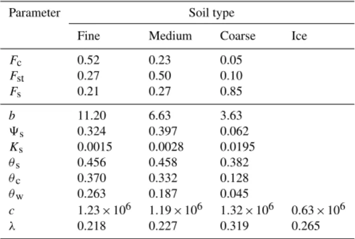
Table 1.JULES soil parameter values for fine, medium and coarse soil used in the Brooks and Corey (1964) soil hydrology scheme.Fc is clay fraction;Fstis silt fraction;Fsis sand fraction, all
dimen-sionless;bis the Brooks-Corey (or Clapp-Hornberger) exponent in soil hydraulic characteristics (–);9sis the absolute value of the soil
matric suction at saturation (m);Ksis the hydraulic conductivity at
saturation (kg m−2s−1);θsis volumetric soil moisture content at saturation (m3water per m3soil);θcis the volumetric soil moisture
content at the critical point (m3m−3)at which soil moisture stress starts to restrict transpiration;θwis volumetric soil moisture content
at the wilting point (m3m−3);cis dry heat capacity (J m−3K−1); λis the dry thermal conductivity (W m−1K−1)
Parameter Soil type
Fine Medium Coarse Ice
Fc 0.52 0.23 0.05
Fst 0.27 0.50 0.10
Fs 0.21 0.27 0.85
b 11.20 6.63 3.63
9s 0.324 0.397 0.062
Ks 0.0015 0.0028 0.0195
θs 0.456 0.458 0.382
θc 0.370 0.332 0.128
θw 0.263 0.187 0.045
c 1.23×10⁶ 1.19×10⁶ 1.32×10⁶ 0.63×10⁶
λ 0.218 0.227 0.319 0.265
for the period July 1982 to December 1995 with a 3-hourly resolution.
WATCH: this dataset was created for the project Water and Global Change (WATCH, Weedon et al., 2010) and is de-rived from the ERA-40 reanalysis product. The reanalysis fields were interpolated to half-degree resolution, corrected for elevation, and monthly adjustments were applied based on gridded observations from the CRU (temperature, diur-nal temperature range, cloud-cover and number of wet days) and GPCC (precipitation) databases. An alternative precipi-tation product based on the CRU observations only was also created but this includes fewer stations than the GPCC data (Weedon et al., 2010). In addition corrections were applied for atmospheric aerosol loading and separate precipitation gauge corrections for rainfall and snowfall. The WATCH forcing data cover the period 1901 to 2001 but in this paper we use an earlier version starting from 1959. The data are provided with 3-hourly time step and at a half-degree reso-lution. The JULES simulations described in this paper that were driven by WATCH primarily use the (standard) GPCC precipitation (WATCH-GPCC) product but we did make a comparison with the CRU precipitation (WATCH-CRU) at a limited number of sites (see Sect. 6).
Table 2. Parameters for organic soil used in the SOC experiment. For explanation of the parameters and units, see Table 1.
Parameter Top layer Layer 2 Layer 3 Source 0–10 cm 10–35 cm 35–100 cm
b 2.7 6.1 12.0 Letts et al. (2000)
9s 0.0103 0.0102 0.0101 Letts et al. (2000)
Ks 0.28 0.002 0.0001 Letts et al. (2000)
θs 0.93 0.88 0.83 Letts et al. (2000)
θc 0.11 0.34 0.51 a
θw 0.03 0.18 0.37 a
c 0.58×10⁶ 0.58×10⁶ 0.58×10⁶ Oke (1987)b
λ 0.06 0.06 0.06 Oke (1987)b
aEstimated following Cosby et al. (1984),bbased on Van Wijk and De Vries (1963).
3.2 Model parameters
In addition to meteorological input, JULES requires informa-tion on vegetainforma-tion fracinforma-tions and soil parameters (see Sect. 2). In our runs we used “standard” input datasets that are also commonly used in Hadley Centre climate model experi-ments. Vegetation types were derived from the International Geosphere Biosphere Programme’s (IGBP) global land cover database1that is based on satellite data from the period April 1992 through March 1993 with a resolution of 1 km. The soil data originally derive from the Wilson and Henderson-Sellers (1985) soils dataset that provides information on soil classes on a global 1-degree grid. Based on fractions of sand, silt and clay for each soil type the soil parameters used in the Clapp and Hornberger (1978) soil hydrology scheme are cal-culated using the equations suggested by Cosby et al. (1984). Typical parameter values obtained in this way are given in Table 1.
In its standard setup (and as used within GCMs), JULES soil parameters are constant with depth and for mineral soils only. However, as many have pointed out (e.g. Beringer et al., 2001; Nicolsky et al., 2007), organic soil behaves very dif-ferently from mineral soil. This is particularly important in the Arctic where mineral soils are often overlain by a layer of peat, mosses or lichens, providing thermal insulation to the lower mineral soil layers (Gornall et al., 2007). Although JULES can be used to simulate the soil carbon cycle, at present it does not include the influence of soil organic mat-ter on the thermodynamic and hydrological properties of the soil. Here we include the results of an experiment in which the standard mineral soil parameters were adjusted accord-ing to soil organic content. This adjustment is similar to that used in other models (e.g. Lawrence and Slater, 2008) and is based on a linear combination of mineral and organic soil properties, according to the organic content. The properties of organic soil are based on Letts et al. (2000) and Oke (1987) and, in contrast to Lawrence and Slater (2008), were allowed
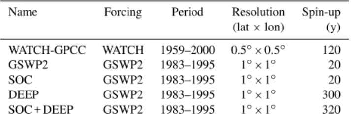
Table 3.JULES Northern Hemisphere grid experiments used in this paper.
Name Forcing Period Resolution Spin-up (lat×lon) (y)
WATCH-GPCC WATCH 1959–2000 0.5◦×0.5◦ 120
GSWP2 GSWP2 1983–1995 1◦×1◦ 20
SOC GSWP2 1983–1995 1◦×1◦ 20
DEEP GSWP2 1983–1995 1◦×1◦ 300
SOC + DEEP GSWP2 1983–1995 1◦×1◦ 320
to vary with depth (see Table 2; note that in Lawrence and Slater (2008) organic content itself does change with depth). Rather than assuming a blanket layer of organic material on top of the soil column (as in e.g. Rinke et al., 2008) we ob-tained data on soil organic content in permafrost regions from the Northern Circumpolar Soil Carbon Database (NCSCD) (Tarnocai et al., 2009). These data were regridded to a 1-degree grid and distributed over the top three model layers. The NCSCD provides soil organic carbon content in kg m−2
over two depths, 0–30 cm and 0–100 cm. The first data were distributed over the top two layers of JULES; the remainder was assigned to the third layer. In the fourth (bottom) model layer the carbon content was assumed to be zero. A max-imum value for soil carbon of 130 kg m−3 (Farouki, 1981) was used to calculate the organic fraction from the actual car-bon content in each layer. This organic fraction then deter-mines the extent that the organic soil properties are allowed to influence the final soil properties: when the organic frac-tion is very low, the soil properties are similar to the original mineral soil parameters. In grid cells with a high organic fraction, the parameters are close to the properties of pure organic soil given in Table 2.
3.3 Model experiments
We ran JULES for the Northern Hemisphere land mass driven by each of the meteorological forcing datasets de-scribed above (see Table 3). In the following, each simu-lation is designated by its forcing, i.e. GSWP2, WATCH. The GSWP2 simulations cover areas north of 25◦N while
WATCH-GPCC was run for areas north of 45◦N, meaning the latter does not include the Qinghai-Tibetan Plateau. In each experiment the grid resolution was kept the same as in the driving dataset, i.e. 1◦×1◦ in the GSWP2 runs and 0.5◦×0.5◦in WATCH-GPCC, maintaining consistency with the forcing. The internal time step in all simulations was 1 h. Before the actual simulation period the model was spun-up by running repeatedly using the meteorological input of the first year, until soil moisture and temperature in each layer reached equilibrium.
The model experiments with extended soil profile (DEEP) and with organic soil parameters (SOC) were run driven by
GSWP2 forcing only. A third experiment combining the two modifications (SOC + DEEP) was also run using GSWP2. In the runs with the extended soil profile a longer spin-up period is required to bring the slow-responding lower soil layers into equilibrium with the climate. To speed up this process, the model was run with an internal time step of 3 h for 300 yr, driven by the climatological average of the GSWP2 forcing over 1983–1995, thus discarding the interannual variability in this period.
Additionally, we performed a number of point-scale simu-lations for comparison with observed soil temperature and moisture content at three soil climate monitoring sites in Alaska. The data was obtained from the United States De-partment of Agriculture (USDA) Natural Resources Con-servation Service (NRCS)2. These runs used site-specific soil parameters (see Table 4) but were driven by the same WATCH global meteorological dataset described above, that we assumed to be the best available, continuous and con-sistent meteorological forcing for these sites. Since JULES does not have a specific tundra plant functional type we as-sumed C3 grass to be the closest approximation of the vege-tation type. At each location the model was first spun up by running repeatedly with the meteorological input of the first year (1959), and then ran continuously to 2001. However, since the soil climate research stations were only established after the mid-1990s, only the latter part of the simulation pe-riod was used for comparison with observations. Two sets of simulations were performed, the first using mineral soil parameters only, comparable to the standard setup in JULES and in the climate models. In the second set of simulations the soil parameters were adjusted for organic carbon content, derived for these locations from the NCSCD database. These runs are thus comparable to the SOC spatial model run, al-though the effect on the soil parameterisation can be expected to be somewhat larger as the organic fractions were not aver-aged out over a larger grid.
4 Results – standard JULES
In the following sections we evaluate the performance of JULES in simulating soil temperatures and active layer thick-ness (ALT) by comparing the results from the GSWP2 and WATCH-GPCC runs with observational datasets. ALT was diagnosed from the simulated soil temperatures by fitting a thermal profile by means of linear interpolation through the midpoints of each soil layer and calculating the depth at which the profile crosses the 0◦C isotherm. Below the mid-point of the bottom layer the position of the thawing front was calculated by extrapolation from above (see Risebor-ough, 2008). This thawing depth was calculated for each day in the simulation period and the annual maximum thaw depth was used as an indicator of the ALT.
2Available from http://soils.usda.gov/survey/smst/alaska/index.
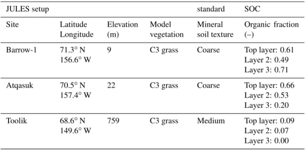
Table 4.JULES point simulations at USDA-NRCS soil climate research sites.
JULES setup standard SOC
Site Latitude Longitude
Elevation (m)
Model vegetation
Mineral soil texture
Organic fraction (–)
Barrow-1 71.3◦N 156.6◦W
9 C3 grass Coarse Top layer: 0.61 Layer 2: 0.49 Layer 3: 0.71
Atqasuk 70.5◦N 157.4◦W
22 C3 grass Coarse Top layer: 0.66 Layer 2: 0.53 Layer 3: 0.20
Toolik 68.6◦N 149.6◦W
759 C3 grass Medium Top layer: 0.09 Layer 2: 0.07 Layer 3: 0.00
Fig. 1. (a)Observed permafrost coverage, as compiled by the Inter-national Permafrost Association (IPA) (Brown et al., 2001);(b)and
(c)Areas with permafrost in the GSWP2 and WATCH runs, respec-tively, with mean active layer thickness (ALT) over the period indi-cated.
4.1 Permafrost extent
Figure 1 shows the extent of permafrost in the JULES simu-lations compared to observed permafrost extent of the Inter-national Permafrost Association (IPA) (Brown et al., 2001). In both runs there is visually a good agreement between the areas with permafrost in JULES and where permafrost is known to occur. The total permafrost area in GSWP2 (based
on areas with an ALT of less than 3 m) is 22.16 million km2, which at first sight corresponds well with other estimates of total hemispheric permafrost extent based on the IPA map of circum-arctic permafrost (see Zhang et al., 2003). However, the IPA classifies areas with permafrost into classes with de-creasing coverage: continuous permafrost (90–100 % cov-erage), discontinuous (50–90 %), sporadic permafrost (10– 50 %), and isolated permafrost patches (less than 10 % cov-erage). JULES, on the other hand, does not account for sub-grid variability in soil temperature, implying that it should only simulate permafrost if the areal coverage is at least 50 %. With this in mind, the model appears to overestimate the areal extent of permafrost.
Table 5.Cross-tabulation of permafrost extent classes in the IPA permafrost map (Brown et al., 2001) and JULES mean ALT classes in the GSWP2 run (1983–1995). The table summarises the total area where each IPA extent class (rows) coincides with each JULES ALT class (columns). IPA areas may differ slightly from previously reported estimates (e.g. Zhang et al., 2003) because of regridding and the different land/sea mask in the JULES modelling grid. Values are in million km2.
IPA extent JULES mean ALT (cm)
<50 <100 <150 <200 <250 <300 no permafr. total
no permafrost 0.22 0.72 0.80 1.54 2.00 3.05
isolated 0.00 0.00 0.01 1.41 1.85 2.37 1.41 3.78 sporadic 0.00 0.00 0.01 2.49 2.87 3.17 0.69 3.87 discontinuous 0.00 0.01 0.17 3.42 3.64 3.72 0.46 4.19 continuous 0.36 4.99 6.92 9.70 9.79 9.84 0.01 9.86
total 0.59 5.73 7.92 18.56 20.16 22.16 2.58 21.69
total in discontinuous + continuous
0.36 5.01 7.10 13.12 13.43 13.57 0.48 14.04
total in isolated + sporadic
0.00 0.00 0.02 3.90 4.73 5.55 2.10 7.65
total in isolated + sporadic + no permafr.
0.22 0.72 0.82 5.44 6.73 8.60 2.10
4.2 Active layer thickness
Observations on active layer thickness have been collected by the Circumpolar Active Layer Monitoring (CALM) since the 1990s (Brown et al., 2000). The network consists of over 100 monitoring sites, most of which are located in arctic and sub-arctic lowlands. There are three primary methods of determining the ALT: by mechanical probing at rectangular grids and/or transects of various size; by employing thaw-tubes; and by inferring the thaw depth from ground temper-ature measurements. Here we compare the annual end-of-season thaw depth from the CALM network3with the ALT in the JULES simulations. Unfortunately there is only a lim-ited overlap between observations and simulations: WATCH-GPCC ends in 2000, and GSWP2 in 1995, and at many sites few observations, if any, are available before then.
In Fig. 2 we compare the simulated ALT (as inferred from soil temperature) with the observed thaw depth for those lo-cations and years where observations are available. Note that ALT was calculated by linear interpolation of the soil temperature between the layer midpoints, which may lead to considerable bias (cf. Riseborough, 2008). It should also be kept in mind that the JULES runs are relatively coarse-scale (1◦×1◦in GSWP2 and 0.5◦×0.5◦in WATCH-GPCC), while the observations are essentially at point-scale or representa-tive of a much smaller area taken by a variety of methods. Also the vertical resolution of these standard simulations is
3 Available from http://www.udel.edu/Geography/calm/index.
html
Fig. 2. Observed and simulated (calculated from soil temperature profiles) active layer thickness (ALT) at CALM observations sites. Values are shown for the period 1990–1995 for the JULES-GSWP2 run, and 1990–2000 for the JULES-WATCH run.
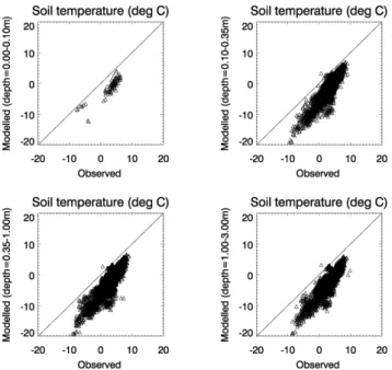
Fig. 3. Simulated and observed mean annual soil temperatures at Russian meteorological stations. Modelled soil temperatures are from the WATCH run (1958–2000) for the level indicated; obser-vations are from depths falling within each corresponding model level.
of the simulated ALT being too deep compared to the ob-served end-of-season thaw depth (Fig. 2). Averaged over all common data pairs, the mean difference in the GSWP2 run is 0.81±0.48 m, and 0.53±0.50 m in WATCH-GPCC. The root mean square error (RMSE) is 0.94 and 0.73 m, respec-tively.
4.3 Soil temperatures
To evaluate JULES simulated soil temperatures in permafrost regions, we used the Russian Historical Soil Temperature dataset4. This dataset is a collection of monthly and annual average soil temperatures measured at Russian meteorolog-ical stations. Data were recovered from many sources and compiled by Zhang et al. (2001). Soil temperatures were measured at depths of 0.02 to 3.2 m using bent stem ther-mometers, extraction therther-mometers, and electrical resistance thermistors. Data coverage extends from the 1800s through 1990 but is not continuous. At many stations data collection began in the 1930s or 1950s, and not all stations continued to take measurements through to 1990.
In Fig. 3 we compare the observed annual mean soil tem-peratures with results from WATCH-GPCC that has a longer overlap with the observations, for those years and stations where observations are available. Simulated soil tempera-tures in each of the four layers are compared with obser-vations pooled for all of the measurement depths that fall
4Available from http://nsidc.org/data/arcss078.html
within these layers. In other words, no interpolation was ap-plied and this may explain some of the differences that can be seen. Nevertheless, it is obvious that the simulated an-nual mean soil temperatures are generally too low compared to the observations, and this bias is larger at colder stations. It is also larger in winter than in summer, as can be seen in Fig. 4 where simulations and observations are compared on a monthly basis. In the top soil the bias is largest in mid-winter (December–February) and smallest towards the end of sum-mer (September–October), when simulations are generally in relatively good agreement with the observations. Deeper in the soil this minimum bias is then shifted to later in the year: at 1.6 m depth, the bias is smallest in November. The GSWP2 experiment (not shown), that has a shorter overlap with the observations, fundamentally shows a similar picture although the cold bias appears to be somewhat less than in WATCH-GPCC.
Because of the mismatch in scale in simulations (0.5◦×
0.5◦)and observations, and the discontinuities in the
obser-vations, there is no straightforward single explanation for the cold bias in the simulated soil temperatures. Generally speaking, JULES captures the attenuation and delay of the seasonal cycle in soil temperature reasonably well. The re-sults seem to suggest the top soil layers are cooling down too much in winter, but note that there are only limited observa-tions available for the top soil in the winter months (see also Fig. 3).
5 Results – modified JULES
ALT compared to standard JULES, although the difference is mostly less than∼20 cm (Fig. 5).
In the DEEP run, the bottom layer is – in places – warmer than the standard setup in spring and early summer, but cooler by the end of summer and in autumn, as more heat is being transferred to warm up the added soil layers below (Fig. 6d). In effect, the seasonal cycle is dampened because of the soil layers underneath. In places where summer thaw-ing reaches the bottom layer, the slightly cooler temperature results in a slightly shallower ALT but the differences are generally very small (Fig. 5b). A peculiar effect that can be seen at the boundaries of the permafrost region is that the deeper soil layers allow a deeper ALT to be calculated that in places extends below the original soil profile of 3 m. There-fore, if we apply the same threshold of an ALT below 3 m to identify grid cells with permafrost the actual permafrost area in DEEP is slightly smaller than in GSWP2.
In both SOC and DEEP the differences from the standard JULES setup are, however, too small to remedy the general overestimation of the ALT compared with the observations at CALM sites that was noted earlier. The RMSE, which was 0.94 m in GSWP2, is only marginally lower: 0.93 m in the SOC experiment, 0.90 m in DEEP, and 0.91 m when both modifications are combined.
6 Results – site-specific runs
To better understand the performance of JULES in cold cli-mate regions we ran a number of point-scale simulations for a number of soil climate research stations in Alaska for which observations on both soil temperature and moisture content were available. These runs were driven by the same WATCH global meteorological forcing datasets that was used in the spatial runs, but used vegetation and soil parameters that were based on the site descriptions (see Table 4). In the fol-lowing we show results for three stations: Toolik (68.6◦N, 149.6◦W, altitude 759 m); Atqasuk (70.5◦N, 157.4◦W, alti-tude 22 m); and Barrow-1 (71.3◦N, 156.6◦W, altitude 9 m), the latter being closest to the coast.
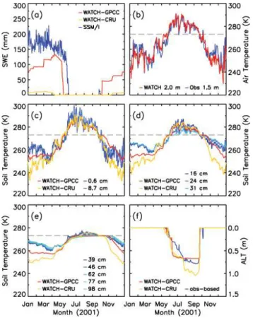
A major limitation when running a complex model like JULES at single sites is the availability of meteorological forcing data with sufficient duration, frequency and qual-ity. Observations at micrometeorological tower sites (such as the FLUXNET sites) often contain gaps and errors, par-ticularly in winter. We tried to circumvent this problem by using global forcing datasets but obviously these have lim-itations as well. This is illustrated in Fig. 7a where the amount of snow (in mm water equivalent, SWE) at Toolik as derived from SSM/I satellite observations5 is compared with the snow mass simulated by JULES driven by the two variants of WATCH – the standard product using the GPCC precipitation data (WATCH-GPCC) and WATCH-CRU that
5Available from the ArcticRIMS website: http://RIMS.unh.edu
is based on a smaller number of precipitation observations. Clearly, the latter of the two datasets considerably underes-timates the amount of cold season precipitation at this lo-cation. Over the 2000–2001 winter season, the total pre-cipitation between October and April in WATCH-CRU is only 16 mm or about 10 % of the amount in WATCH-GPCC. As a consequence, the model simulates only a very shallow snow pack that disappears too early in spring. The WATCH dataset using the GPCC precipitation, which is based on a larger number of stations than CRU, performs much better in this respect and the simulated amount of snow is much closer to the satellite-derived SWE, although the snow vol-ume is still lower and disappears about half a month ear-lier. The latter is at least partly due to the WATCH forc-ing beforc-ing somewhat warmer than observed at Toolik in the weeks preceding snowmelt, with daytime temperature fre-quently climbing above zero degrees Celsius from early May onwards (Fig. 7b). Note that in general there are also un-certainties associated with satellite-based estimates of SWE, especially at high values. The observed snow depth at Toolik at 2 May 2001 (Oberbauer, 2003) amounted to 0.66 m with a standard deviation of 0.09 m. Assuming a snow density in the range of 260–310 kg m−3(e.g. Sturm and Wagner, 2010) this translates into a SWE of 172–205±28 mm. The SSM/I estimate on this day is 181 mm but day-to-day variability in these data is considerable with values as low as 125 mm in the 10 days around the measurement date. JULES, using a prognostic snow density, calculates a snow depth on this day of 0.30 m and an SWE of 115 mm when using the WATCH-GPCC forcing.
These differences in snow mass have an impact on the simulated soil temperatures (Fig. 7c–e) and calculated thaw depth (Fig. 7f). Compared to WATCH-CRU, the deeper snow pack in WATCH-GPCC leads to higher temperatures in the top soil, but primarily so in autumn and winter. In spring, on the other hand, the thin snow cover and its earlier depletion in WATCH-CRU allows the top soil temperatures to rise more quickly from its colder state, while in summer both runs are in close agreement and correspond relatively well with the observed soil temperatures (Fig. 7c, d). In the subsoil, GPCC is generally warmer than CRU except for about 2 months in (late) summer (Fig. 7e). In the deepest soil layer the differ-ence between GPCC and CRU persists throughout the year but is smallest in late autumn. Note that in WATCH-GPCC the top soil temperatures in winter are still lower than ob-served while the air temperature (which is the same in both WATCH variants) is mostly in good agreement with the ob-servations at this site (Fig. 7b).
Fig. 4.As Fig. 3 but averaged over all months and stations to show the mean annual cycle.
inferred from temperature measurements on the day of prob-ing is∼0.75 m. Although this is considerably deeper, it still falls within the total range of the observations (0.21–0.88 m), highlighting the high spatial variability in active layer thick-ness, which reflects the local influence of vegetation, sub-strate properties, snow cover dynamics and terrain (Hinkel and Nelson, 2003).
In spite of the much colder soil temperatures in winter, the maximum thaw depth in the WATCH-CRU simulation is con-siderably deeper than in WATCH-GPCC (1.04 m vs. 0.67 m,
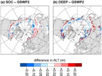
Fig. 5. Difference in mean ALT over 1983–1995 between the GSWP2 run (standard JULES) (cf. Fig. 1) and(a)SOC (JULES with soil parameters modified according to organic content); and
(b)DEEP (JULES with soil profile extended to 60 m depth). Note positive values (red colours) signify the mean ALT is deeper in the modified setups than in GSWP2, negative values (blue) means it is shallower.
affect the simulation of soil temperature and consequently the calculation of the thawing depth.
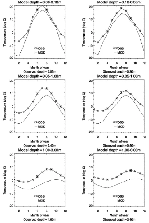
In Fig. 8 we compare simulated soil temperature and mois-ture content with observations at Atqasuk for the year 2000. Note in these plots the meteorological forcing in the two sim-ulations is the same (WATCH-GPCC) but the soil parameter values are different: the standard simulation assumes homo-geneous mineral soil parameters, in the SOC simulation these are adjusted for organic carbon content. The JULES soil moisture shown in Fig. 8 is the unfrozen moisture fraction rather than the total soil moisture, as this was assumed to be directly comparable to the observations. The soil moisture measurements are given in water fraction by volume (wfv), meaning that at values around 0.40–0.45 the soil is fully sat-urated, dependent on the porosity. JULES soil moisture was converted to wfv using the porosity values of the soil type used in the simulation. For those layers where observations are available (layer 2: 10–35 cm, and layer 3: 35–100 cm) they suggest the soil is close to saturation throughout sum-mer up to a depth of at least 50 cm (Fig. 8e, f). No deeper observations are available but the temperature measurements indicate that below this depth the soil remains frozen. In the model, the second soil layer thaws completely and the un-frozen moisture fraction in summer reflects the total mois-ture content. This layer is too dry in summer, especially in standard setup using mineral soil parameters. In layer 3 on the other hand, the total moisture content in both sim-ulations is close to saturation throughout the year but most of it remains frozen. In both layers the absolute amount of soil water is larger in the SOC experiment that has a higher
porosity than the mineral soil in the standard setup, affect-ing the simulation of soil temperatures. Because the larger amount of water requires more time to melt, the temperature in layer 2 remains isothermal at 0◦C for a longer period of time, which subsequently affects the penetration of the thaw-ing front into the soil (Fig. 8h). However, the overall ef-fect of the SOC parameterisation on the deeper soil tempera-tures, as well as the maximum thaw depth that is reached, appears to be minimal. The reported end-of-season thaw depth in the CALM database for Atqasuk in 2000 (averaged over 105 observations) amounts to 0.43±0.20 m. Calculated from observed soil temperature, the maximum seasonal thaw depth is 0.45 m. In the JULES simulations, this is 0.63 m and 0.58 m with the standard and SOC setups, respectively. The JULES ALT estimates are therefore considerably deeper but still within one standard deviation from the average across the CALM observation grid.
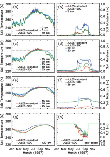
Similar patterns can also be observed in Barrow (Fig. 9), where observations on soil moisture content are also avail-able for the top soil. Both JULES simulations capture the temporal variation in top soil moisture reasonably well, but appear too dry compared to the measurements (Fig. 9b). An interesting feature that can be observed at both Atqasuk and Barrow is that the top three model layers are cooling down more rapidly in autumn than observed. The observations remain isothermal close to 0◦C for an extended period of time, in some years until November, suggesting the freez-ing of soil water is slower than simulated by the model. The opposite sometimes happens in spring, when the model re-mains close to melting longer than the observations, espe-cially in the SOC runs that have higher moisture content (cf. Fig. 8c). Throughout the rest of the year the difference in soil temperature between the two model setups remains very small. In Fig. 9h the maximum thaw depth in the two sim-ulations (standard: 0.63 m, SOC: 0.55 m) is also close to the ALT derived from soil temperature measurements (0.61 m). In the CALM database, the observed ALT at Barrrow in 1997 ranges between 0.21 and 0.75 m with an average of 0.39±0.09 m.
7 Discussion
Fig. 6. Simulated mean soil temperature in GSWP2 (standard JULES) and difference with GSWP2 in the DEEP (extended soil profile) and SOC (modified soil parameters) experiments, averaged over a permafrost area in Siberia (110–135◦E, 60–70◦N):(a)top soil layer (0–10 cm);(b)layer 2 (10–35 cm);(c)layer 3 (35–100 cm);(d)bottom layer (100–300 cm). Note the temperature difference from GSWP2 in the DEEP and SOC runs is shown on the right-hand axes.
with the IPA permafrost map; in other words, JULES simu-lates permafrost where it is known to occur. However, it can be argued that the model overestimates the total permafrost extent, as it simulates permafrost also in those areas where it occurs sporadically (areal coverage less than 50 %) or even only in isolated patches. In a way one could say JULES sim-ulates the potential upper limit of large-scale permafrost oc-currence rather than the actual coverage that also depends on local conditions.
Consistent with this overestimation of the total permafrost extent is a general cold bias in soil temperatures that was found when comparing JULES with observations at a large number of stations in Russia (Figs. 3 and 4) and, to a lesser extent, also in Alaska (Figs. 7–9). Especially in winter the simulated soil temperatures are considerably lower than ob-served, something that has also been found in other LSMs (e.g. Nicolsky et al., 2007). PaiMazumder et al. (2008) on the other hand, found that the simulated soil temperatures in the fully coupled Community Climate System Model (CCSM) were mostly too high in winter when compared with the Russian station data, which was attributed to an overestima-tion of winter precipitaoverestima-tion and consequently snow depth by CCSM. One possible explanation for the cold bias found in JULES is therefore that the snow cover in the model provides too little thermal insulation against low winter temperatures. The simulations at Toolik in Alaska (Fig. 7) demonstrate that
at this location the low soil temperatures in winter can at least partly be remedied with better precipitation input yielding a deeper snow pack. In this respect it is worth noting that solid winter precipitation measurements are highly uncertain (Goodison et al., 1998; Yang and Woo, 1999). The GSWP2 and WATCH-GPCC datasets used in our model runs both correct for gauge undercatch but some bias is still likely over many areas, resulting in a snow pack that is often too thin. Alternatively, the effective thermal capacity of the modelled snow layers might be too low and/or the thermal conductivity too high. Further evaluation of the snow model in JULES and its ability to represent the hydrology of high-latitude regions is therefore required (see also Haddeland et al., 2011).
Uncertainties in the precipitation input also affect soil temperatures by changing the moisture content of the soil. In JULES and similar LSMs the soil thermodynamics are tightly coupled to the hydrology, and this is especially im-portant where phase changes are involved. Differences in soil moisture particularly influence the propagation of the thaw-ing front in summer, and because of the relatively coarse ver-tical resolution of the deeper soil layers, small differences in temperature around the melting point may have a large im-pact on the calculated thaw depth (cf. Fig. 7).
Fig. 7. Simulated snow mass, air and soil temperature and thaw depth at Toolik, Alaska in 2001 using two versions of the WATCH forcing data (based on GPCC and CRU precipitation) com-pared with observations:(a)snow water equivalent (SWE) derived from SSM/I satellite data (available from the ArcticRIMS project);
(b)air temperature at 2.0 m (WATCH forcing) and 1.5 m (observed);
(c)soil temperature in the top model layer (0–10 cm),(d)second layer (10–35 cm), and(e)third layer (35–100 cm); (f)thaw depth or active layer thickness (ALT) calculated from the soil temperature profiles. Soil temperature observations are indicated by their depth of measurement.
53 cm in WATCH (Fig. 2). At first sight this finding may ap-pear contradictory to the cold bias in simulated soil tempera-tures, as it suggests the soil temperatures in the model are too warm, allowing the thawing front to penetrate too much into the frozen soil. It should be kept in mind though that the sim-ulated temperature is in much better agreement with the ob-servations in summer and, deeper in the ground, in autumn. The depth of the active layer provides a measure of the cumu-lative thermal history of the ground surface during the sum-mer thaw period and is highly sensitive to land-atmosphere exchanges. When the ALT is determined from observed tem-perature profiles, the difference with the simulations is more consistent with the differences in soil temperature. More so, the thaw depth in the model also depends on soil moisture content and the associated phase changes. As long as the frozen moisture fraction has not melted completely, the cor-responding model layer remains isothermal around 0◦C and
Fig. 8. Simulated soil temperature(a, c, e, g), soil moisture con-tent(b, d, f)and thaw depth(h)at Atqasuk, Alaska in 2000 with standard and adjusted (SOC) soil parameters compared with obser-vations:(a, b)top model layer (0–10 cm);(c, d)second layer (10– 35 cm);(e, f)third layer (35–100 cm);(g)bottom model layer (1.0– 3.0 m);(h)active layer thickness calculated from soil temperature profiles. Observations are indicated by their depth of measurement, soil moisture content is fraction of total volume.
Fig. 9.As Fig. 8 but for Barrow, Alaska in 1997.
GSWP2 run (i.e. with homogeneous mineral soil parame-ters) but in which the soil column was divided into 30 lay-ers of 10 cm each. Because of the additional computation cost such a setup is unlikely to be adopted in climate model simulations but in offline experiments this approach may be feasible. The results of this experiment are summarised in Fig. 10. Compared to the standard setup of four layers, the higher vertical resolution leads to a more differentiated ALT. Deeper thaw depths are simulated mainly towards the south-ern fringe of the permafrost but further north and especially in large parts of Siberia the ALT becomes shallower. At the CALM sites (Fig. 10c) the average difference with the re-ported end-of-season thaw depth reduces from 0.81±0.48 m to 0.58±0.40 m (RSME from 0.94 to 0.71 m), but a consid-erable bias still remains. A higher vertical resolution is thus beneficial for the simulation of thaw depth in permafrost re-gions but cannot solve completely the general tendency to overestimate the ALT. In either case it should be kept in mind that uncertainties are very large since we are compar-ing point-scale observations, reflectcompar-ing local scale climato-logical conditions and soil properties, with grid-scale simu-lations driven by global datasets. As noted before, the small-scale variability in ALT can be very high resulting in a wide
Fig. 10. (a)Mean ALT over 1983–1995 in a GSWP2 run with the soil column divided in 30 layers of 10 cm (cf. Fig. 1);(b)difference in ALT with the standard setup of four layers; and(c)comparison of simulated ALT from both runs with observations at CALM sites (cf. Fig. 2). Colours in(b) are as in Fig. 5 but note the scale is different.
also find a lowering of the soil temperatures in the top three layers of the model in summer but mostly warmer tempera-tures in winter, as the lower thermal conductivity provides a better protection against the winter cold. On an annual basis, the net effect is therefore fairly small, the difference usually being less than 1◦C, with slightly colder temperatures in the top soil layers and mostly somewhat warmer conditions in the subsoil (layer 3) and bottom layer of the model. For com-parison, Lawrence and Slater (2008) mention up to 2.5◦C cooler annual mean soil temperatures, Rinke et al. (2008) found a reduction in ground temperature by 0.5 to 8◦C.
The limited influence of soil organic material that we find is partly the result of regridding the original NCSCD to a rather coarse 1-degree grid, with the consequence of organic content, which locally can be very high, being averaged out over a much larger area. As a result, the organic fraction in most grid boxes is considerably less than the assumed maxi-mum of 130 kg m−3, especially in the deeper soil layers, and
the final soil properties are still, to a large extent, influenced by the mineral soil. In our simulations the organic fraction in the top soil was nowhere higher than 0.7, and averaged over the domain covered by the NCSCD more in the order of 0.3. A better approach would therefore be to allow for sub-grid variation in soil properties, similar to the sub-grid vegetation tiles that are already used in JULES. Allowing for such sub-grid variability would give the opportunity to represent soils with a higher organic content or even purely organic soils, and it would also enable JULES to estimate fractional per-mafrost coverage within a given grid box. Alternatively, one could opt for adopting a higher resolution in the simulations in order to better represent the spatial variability of the land-scape. However, in relatively complex LSMs like JULES there is always a trade-off to be made between the level of detail that can be included in representing the land surface, and the computation time it takes to run the model. This is especially important when used as a land surface scheme in climate model simulations.
Over all, we find that JULES has some skill in simulat-ing the large-scale characteristics of permafrost but further work is necessary to reduce the cold bias in the simulated soil temperatures, especially during winter. For a better simula-tion of the ALT a higher vertical resolusimula-tion and extended soil profile will be beneficial. Future model development should ensure a dynamic coupling of soil organic carbon content and soil thermal and hydraulic properties (Falloon et al., 2011), as well as allowing for sub-grid variability and uncertainty in soil properties. A separate peat module for JULES is al-ready under development in order to study peatland carbon dynamics in the boreal zone, and work is underway to cou-ple JULES to a more advanced model of carbon and nitro-gen turnover in both mineral and organic soils (Smith et al., 2010).
8 Conclusions
When driven by observation-based climatology, JULES is able to represent the large-scale distribution of circumpolar permafrost reasonably well. The model simulates permafrost where it is known to occur and captures more than 95 % of the continuous and discontinuous (more than 50 % spatial coverage) permafrost. However, the total extent appears to be overestimated as JULES also simulates permafrost in ar-eas where the spatial coverage is sporadic (less than 50 %) or even in isolated patches only. Consistent with this we find a general cold bias in the simulated soil temperatures when compared with observations, especially in winter. This may partly be the result of biases in the model forcing data. Un-certainties in the precipitation input affect the simulation of soil temperatures in two ways: by affecting the thickness of the snowpack and therefore the amount of thermal insulation in winter; and by changing the amount of water in the soil which, because of the energy required for phase changes, af-fects the thermodynamics of soil layers close to the freezing point of water. In turn this affects the simulation of thaw depth and ALT. Generally speaking the model appears to overestimate the annual maximum thaw depth, which can at least partly be explained by the relatively coarse vertical resolution in its standard setup, with the bottom layer span-ning over 2 m. However, uncertainties in the observations are large as ALT is highly variable over small scales.
Acknowledgements. The work described in this paper was sup-ported by the Joint DECC/Defra Met Office Hadley Centre Climate Programme (GA01101), the European Union 6th Framework Programme Integrated Project Water and Global Change (WATCH) (Contract 036946), and the Foreign & Commonwealth Office’s (FCO) Strategic Programme Fund. The authors would like to thank Andy Wiltshire and Douglas Clark for their assistance with JULES, and Pete Falloon for his comments on an earlier version of this paper.
Edited by: D. Riseborough
References
Alexeev, V. A., Nicolsky, D. J., Romanovsky, V. E., and Lawrence, D. M.: An evaluation of deep soil configurations in the CLM3 for improved representation of permafrost, Geophys. Res. Lett., 34, L09502, doi:10.1029/2007GL029536, 2007.
Anisimov, O. A.: Potential feedback of thawing permafrost to the global climate system through methane emission, Environ. Res. Lett., 2, 045016, doi:10.1088/1748-9326/2/4/045016, 2007. Anisimov, O. A.: Stochastic modelling of the active-layer
thick-ness under conditions of the current and future climate, Earth’s Cryosphere, 3, 36–44, 2009.
Anisimov, O. A., Shiklomanov, N. I., and Nelson, F. E.: Vari-ability of seasonal thaw depth in permafrost regions: a stochastic modeling approach, Ecol. Model., 153(3), 217–227, doi:10.1016/S0304-3800(02)00016-9, 2002.
Beringer, J., Lynch, A. H., Chapin III, F. S., Mack, M., and Bonan, G. B.: The representation of Arctic soils in the Land Surface Model (LSM): The importance of mosses, J. Climate, 14, 3324– 3335, 2001.
Best, M. J., Pryor, M., Clark, D. B., Rooney, G. G., Essery, R .L. H., M´enard, C. B., Edwards, J. M., Hendry, M. A., Porson, A., Gedney, N., Mercado, L. M., Sitch, S., Blyth, E., Boucher, O., Cox, P. M., Grimmond, C. S. B., and Harding, R. J.: The Joint UK Land Environment Simulator (JULES), model description – Part 1: Energy and water fluxes, Geosci. Model Dev., 4, 677– 699, doi:10.5194/gmd-4-677-2011, 2011.
Betts, R.: Implications of land ecosystem-atmosphere interac-tions for strategies for climate change adaptation and mitigation, Tellus B, 59, 602–615, doi:10.1111/j.1600-0889.2007.00284.x, 2007.
Blyth, E., Best, M., Cox, P., Essery, R., Boucher, O., Harding, R., Prentice, C., Vidale, P. L., and Woodward, I.: JULES: a new community land surface model, Global Change NewsLetter, 66, 9–11, 2006.
Blyth, E., Gash, J., Lloyd, A., Pryor, M., Weedon, G. P., and Shut-tleworth, J.: Evaluating the JULES land surface model energy fluxes using FLUXNET data, J. Hydrometeorol., 11, 509–519, doi:10.1175/2009JHM1183.1, 2010.
Brooks, R. H. and Corey, A. T.: Hydraulic properties of porous media, Colorado State University Hydrology Papers, 3, 1964. Brown, J., Nelson, F. E., and Hinkel, K. M.: The circumpolar active
layer monitoring (CALM) program: research designs and initial results, Polar Geography, 3, 165–258, 2000.
Brown, J., Ferrians Jr., O. J., Heginbottom, J. A., and Melnikov, E. S.: Circum-Arctic map of permafrost and ground-ice con-ditions, National Snow and Ice Data Center/World Data Cen-ter for Glaciology, Boulder, CO, Digital Media, available at: http://nsidc.org, 2001.
Christensen, J. H., Hewitson, B., Busuioc, A., Chen, A., Gao, X., Held, I., Jones, R., Kolli, R. K., Kwon, W.-T., Laprise, R., Maga˜na Rueda, V., Mearns, L., Men´endez, C. G., R¨ais¨anen, J., Rinke, A., Sarr, A., and Whetton, P.: Regional Climate Projec-tions, in: Climate Change 2007: The Physical Science Basis. Contribution of Working Group I to the Fourth Assessment Re-port of the Intergovernmental Panel on Climate Change, edited by: Solomon, S., Qin, D., Manning, M., Chen, Z., Marquis, M., Averyt, K. B., Tignor, M., and Miller, H. L., Cambridge Uni-versity Press, Cambridge, United Kingdom and New York, NY, USA, 847–940, 2007.
Clapp, R. B. and Hornberger, G. M.: Empirical equations for some soil hydraulic properties, Water Resour. Res., 14, 601–604, 1978. Cosby, B. J., Hornberger, G. M., Clapp, R. B., and Ginn, T. R.: A statistical exploration of the relationships of soil moisture char-acteristics to the physical properties of soils, Water Resour. Res., 20, 682–690, 1984.
Cox, P. M., Betts, R. A., Bunton, C. B., Essery, R. L. H., Rowntree, P. R., and Smith, J.: The impact of new land surface physics on the GCM simulation of climate and climate sensitivity, Clim. Dynam., 15, 183–203, 1999.
Dadson, S. J., Ashpole, I., Harris, P., Davies, H. N., Clark D.
B., Blyth, E., and Taylor, C. M.: Wetland inundation dy-namics in a model of land surface climate: Evaluation in the Niger inland delta region, J. Geophys. Res., 115, D23114, doi:10.1029/2010JD014474, 2010.
Dankers, R., Anisimov, O., Kokorev, V., Falloon, P., Reneva, S., and Strelchenko, J.: Permafrost, soil-carbon balance and sus-tainability under climate change, UK-Russia Climate Change Science Collaboration Project Final Report, available at: http: //www.uk-russia-ccproject.info/, 2010.
Dirmeyer, P. A., Gao, X., Zhao, M., Guo, Z., Oki, T., and Hanasaki, N.: The Second Global Soil Wetness Project (GSWP-2): Multi-Model Analysis and Implications for our Perception of the Land Surface, COLA Techn. Rep. 185, available at: ftp://grads.iges. org/pub/ctr/ctr 185.pdf, 2005.
Elberling, B., Christiansen, H. H., and Hansen, B. U.: High nitrous oxide production from thawing permafrost, Nat. Geosci., 3, 332– 335, doi:10.1038/ngeo803, 2010.
Essery, R., Best, M., and Cox, P.: MOSES 2.2 Technical Docu-mentation, Hadley Centre Tech. Note 30, Bracknell: Met Office Hadley Centre, 2001.
Falloon, P., Jones, C. D., Ades, M., and Paul, K.: Direct soil mois-ture controls of fumois-ture global soil carbon changes – an impor-tant source of uncertainty, Global Biogeochem. Cy., 25, GB3010, doi:10.1029/2010GB003938, 2011.
Farouki, O. T.: The thermal properties of soils in cold regions, Cold Reg. Sci. Technol., 5, 67–75, 1981.
Goodison, B. E., Louie, P. Y. T., and Yang, D.: WMO solid precip-itation measurement intercomparison, final report, WMO Instru-ments and Observing Methods Report 67, WMO/TD-No.872, 1998.
Gornall, J. L., J´onsd´ottir, I. S., Woodin, S. J., and Van der Wal, R.: Arctic mosses govern below-ground environment and ecosystem processes, Oecologia, 153, 931–941, doi:10.1007/s00442-007-0785-0, 2007.
Haddeland, I., Clark, D. B., Franssen, W., Ludwig, F., Voß, F., Arnell, N. W., Bertrand, N., Best, M., Folwell, S., Gerten, D., Gomes, S., Gosling, S. N., Hagemann, S., Hanasaki, N., Hard-ing, R., Heinke, J., Kabat, P., Koirala, S., Oki, T., Polcher, J., Stacke, T., Viterbo, P., Weedon, G. P., and Yeh, P.: Multi-model estimate of the global terrestrial water balance: setup and first re-sults, J. Hydrometeorol., doi:10.1175/2011JHM1324.1, in press, 2011.
Hinkel, K. M. and Nelson, F. E.: Spatial and temporal patterns of active layer thickness at Circumpolar Active Layer Monitoring (CALM) sites in northern Alaska, 1995–2000, J. Geophys. Res., 108, 8168, doi:10.1029/2001JD000927, 2003.
Kattsov, V. M., K¨all´en, E., Cattle, H., Christensen, J., Drange, H., Hanssen-Bauer, I., J´ohannesen, T., Karol, I., R¨ais¨anen, J., Svens-son, G., and Vavulin, S.: Future climate change: modeling and scenarios for the Arctic, in: Arctic Climate Impact Assessment, Cambridge University Press, Cambridge, 99–150, 2005. Lawrence, D. M. and Slater, A. G.: A projection of severe near
surface permafrost degradation during the 21st century, Geophys. Res. Lett., 32, L24401, doi:10.1029/2005GL025080, 2005. Lawrence, D. M. and Slater A. G.: Incorporating organic soil
into a global climate model, Clim. Dynam., 30, 145–160, doi:10.1007/s00382-007-0278-1, 2008.
permafrost degradation to soil column depth and representa-tion of soil organic matter, J. Geophys. Res., 113, F02011, doi:10.1029/2007JF000883, 2008.
Letts, M. G., Roulet, N. T., Comer, N. T., Skarupa, M. R., and Verseghy, D. L.: Parametrization of Peatland Hydraulic Proper-ties for the Canadian Land Surface Scheme, Atmos. Ocean, 38, 141–160, 2000.
Nicolsky, D. J., Romanovsky, V. E., Alexeev, V. A., and Lawrence, D. M.: Improved modelling of permafrost dynamics in a GCM land-surface scheme, Geophys. Res. Lett., 34, L08501, doi:10.1029/2007GL029525, 2007.
Nijssen, B., Bowling, L. C., Lettenmaier, D. P., Clark, D. B., El Maayar, M., Essery, R., Goers, S., Gusev, Y. M., Habets, F., Van den Hurk, B., Jin, J., Kahan, D., Lohmann, D., Ma, X., Ma-hanama, S., Mocko, D., Nasonova, O., Niu, G.-Y., Samuelsson, P., Shmakin, A. B., Takata, K., Verseghy, D., Viterbo, P., Xia, Y., Xue, Y., and Yang, Z.-L.: Simulation of high latitude hydro-logical processes in the Torne-Kalix basin: PILPS Phase 2(e): 2: Comparison of model results with observations, Global Planet. Change, 38, 31–53, doi:10.1016/S0921-8181(03)00004-3, 2003. Oberbauer, S. F.: Snow Depth Yearly Measurements at Toolik Sta-tion 1995–2001. Boulder, CO: NaSta-tional Center for Atmospheric Research, ARCSS Data Archive, available at: http://data.eol. ucar.edu/codiac/dss/id=106.ARCSS910, 2003.
Oke, T. R.: Boundary layer climates, Methuen, London, 1987. PaiMazumder, D., Miller, J., Li, Z., Walsh, J. E., Etringer, A.,
McCreight, J., Zhang, T., and M¨olders, N.: Evaluation of Community Climate System Model soil temperatures using ob-servations from Russia, Theor. Appl. Climatol., 94, 187–213, doi:10.1007/s00704-007-0350-0, 2008.
Richards, L. A.: Capillary Conduction of Liquids through Porous Mediums, Physics, 1, 318–333, 1931.
Rinke, A., Kuhry, P., and Dethloff, K.: Importance of a soil organic layer for Arctic climate: A sensitivity study with an Arctic RCM, Geophys. Res. Lett., 35, L13709, doi:10.1029/2008GL034052, 2008.
Riseborough, D. W.: Estimating active layer and talik thickness from temperature data: implications from modeling results, in: Proceedings of the Ninth International Conference on Per-mafrost, Fairbanks, Alaska, 29 July–3 August 2008, edited by: Kane, D. L. and Hinkel, K. M., 2, 1487–1492, 2008.
Riseborough, D., Shiklomanov, N., Etzelm¨uller, B., Gruber, S., and Marchenko, S.: Recent Advances in Permafrost Modelling, Per-mafrost Periglac., 19, 137–156, doi:10.1002/ppp.615, 2008. Rutter, N., Essery, R., Pomeroy, J., Altimir, N., Andreadis, K.,
Baker, I., Barr, A., Bartlett, P., Boone, A., Deng, H., Douville, H., Dutra, E., Elder, K., Ellis, C., Feng, X., Gelfan, A., Goodbody, A., Gusev, Y., Gustafsson, D., Hellstr¨om, R., Hirabayashi, Y., Hi-rota, T., Jonas, T., Koren, V., Kuragina, A., Lettenmaier, D., Li, W.-P., Luce, C., Martin, E., Nasonova, O., Pumpanen, J., Pyles, R. D., Samuelsson, P., Sandells, M., Sch¨adler, G., Shmakin, A., Smirnova, T. G., St¨ahli, M., St¨ockli, R., Strasser, U., Su, H., Suzuki, K., Takata, K., Tanaka, K., Thompson, E., Vesala, T., Viterbo, P., Wiltshire, A., Xia, K., Xue, Y., and Yamazaki, T.: Evaluation of forest snow processes models (SnowMIP2), J. Geophys. Res., 114, D06111, doi:10.1029/2008JD011063, 2009. Sazonova, T. S. and Romanovsky, V. E.: A model for regional-scale estimation of temporal and spatial variability of active layer thickness and mean annual ground temperatures, Permafrost
Periglac., 14, 125–139, doi:10.1002/ppp.449, 2003.
Schuur, E. A. G., Bockheim, J., Canadell, J. G., Euskirchen, E., Field, C. B., Goryachkin, S. V., Hagemann, S., Kuhry, P., Lafleur, P. M., Lee, H., Mazhitova, G., Nelson, F. E., Rinke, A., Ro-manovsky, V. E., Shiklomanov, N., Tarnocai, C., Venevsky. S., Vogel, J. G., and Zimov, S. A.: Vulnerability of Permafrost Car-bon to Climate Change: Implications for the Global CarCar-bon Cy-cle, BioScience, 58, 701–714, doi:10.1641/B580807, 2008. Slater, A. G., Schlosser, C. A., Desborough, C. E., Pitman, A. J.,
Henderson-Sellers, A., Robock, A., Vinnikov, K. Y., Entin, J., Mitchell, K., Chen, F., Boone, A., Etchevers, P., Habets, F., Noil-han, J., Braden, H., Cox, P. M., de Rosnay, P., Dickinson, R. E., Yang, Z.-L., Dai, Y.-J., Zeng, Q., Duan, Q., Koren, V., Schaake, S., Gedney, N., Gusev, Y. M., Nasonova, O. N., Kim, J., Kowal-czyk, E. A., Shmakin, A. B., Smirnova, T. G., Verseghy, D., Wet-zel, P., and Xue, Y.: The representation of snow in land-surface schemes: Results from PILPS 2 (d), J. Hydrometeorol., 2, 7–25, 2001.
Smith, L. C., Sheng, Y., MacDonald, G. M., and Hinzman, L. D.: Disappearing Arctic Lakes, Science, 308, 1429, doi:10.1126/science.1108142, 2005.
Smith, J., Gottschalk, P., Bellarby, J., Chapman, S., Lilly, A., Tow-ers, W., Bell, J., Coleman, K., Nayak, D., Richards, M., Hillier, J., Flynn, H., Wattenbach, M., Aitkenhead, M., Yeluripati, J., Farmer, J., Milne, R., Thomson, A., Evans, C., Whitmore, A., Falloon, P., and Smith, P.: Estimating changes in Scottish soil carbon stocks using ECOSSE. I. Model description and uncer-tainties, Clim. Res., 45, 179–192, doi:10.3354/cr00899, 2010. Stendel, M. and Christensen, J. H.: Impact of global warming on
permafrost conditions in a coupled GCM, Geophys. Res. Lett., 29, 1632, doi:10.1029/2001GL014345, 2002.
Stendel, M., Romanovsky, V. E., Christensen, J. H., and Sazonova, T.: Using dynamical downscaling to close the gap between global change scenarios and local per-mafrost dynamics, Global Planet. Change, 56, 203–214, doi:10.1016/j.gloplacha.2006.07.014, 2007.
Sturm, M. and Wagner, A. M.: Using repeated patterns in snow distribution modeling: An Arctic example, Water Resour. Res., 46, W12549, doi:10.1029/2010WR009434, 2010.
Sturm, M., McFadden, J. P., Liston, G. E, Chapin III, F. S., Racine, C. H., and Holmgren, J.: Snow-shrub interactions in Arctic tun-dra: A hypothesis with climatic implications, J. Climate, 14, 336–344, 2001.
Tarnocai, C., Canadell, J. G., Schuur, E. A. G., Kuhry, P., Mazhi-tova, G., and Zimov, S.: Soil organic carbon pools in the north-ern circumpolar permafrost region, Global Biogeochem. Cy., 23, GB2023, doi:10.1029/2008GB003327, 2009.
Van den Hoof, C., Hanert, E., and Vidale, P. L.: Simulating dy-namic crop growth with an adapted land surface model – JULES-SUCROS: Model development and validation, Agr. Forest Mete-orol., 151, 137–153, doi:10.1016/j.agrformet.2010.09.011, 2011. Van Wijk, W. R. and De Vries, D. A.: Thermal properties of soils, in: Physics of plant environment, edited by: Van Wijk, W. R., John Wiley & Sons: New York, 210–235, 1963.
Walter, K. M., Smith, L. C., and Chapin III, F. S.: Methane bub-bling from northern lakes: present and future contributions to the global methane budget, Philos. T. R. Soc. A, 365, 1657–1676, doi:10.1098/rsta.2007.2036, 2007.
Bellouin, N., Boucher, O., and Best, M.: The WATCH forc-ing data 1958-2001: a meteorological forcforc-ing dataset for land surface- and hydrological-models, WATCH Technical Report 22, available at: http://www.eu-watch.org/, 2010.
Williams, P. and Smith, M.: The Frozen Earth, Cambridge Univer-sity Press, Cambridge, 1989.
Wilson, M. F. and Henderson-Sellers, A.: A global archive of land cover and soils data for use in general circulation climate models, J. Climatol., 5, 119–143, 1985.
Yang, D. and Woo, M.-K.: Representativeness of local snow data for large scale hydrologic investigations, Hydrol. Process., 13, 1977–1988, 1999.
Zhang, T., Barry, R., and Gilichinsky, D. (Compilers): Russian his-torical soil temperature data, National Snow and Ice Data Cen-ter/World Data Center for Glaciology, Boulder, CO, Digital Me-dia, available at: http://nsidc.org, 2001.
Zhang, T., Barry, R. G., Knowles, K., Ling, F., and Armstrong, R. L.: Distribution of seasonally and perennially frozen ground in the Northern Hemisphere, in: Permafrost, edited by: Phillips, M., Springman, S. M., and Arenson, L. U., Swets & Zeitlinger, Lisse, 1289–1294, 2003.
Zhang, Y., Chen, W., and Riseborough, D. W.: Transient projec-tions of permafrost distribution in Canada during the 21st cen-tury under scenarios of climate change, Global Planet. Change, 60, 443–456, doi:10.1016/j.gloplacha.2007.05.003, 2008. Zimov, S. A., Schuur, E. A. G., and Chapin III, F. S.: