Including Correlation in Size, Space, Time and between
Species from Research Survey Data
J. Rasmus Nielsen*., Kasper Kristensen., Peter Lewy., Francois Bastardie
Technical University of Denmark, National Institute of Aquatic Resources (DTU AQUA), Charlottenlund, Denmark
Abstract
Trawl survey data with high spatial and seasonal coverage were analysed using a variant of the Log Gaussian Cox Process (LGCP) statistical model to estimate unbiased relative fish densities. The model estimates correlations between observations according to time, space, and fish size and includes zero observations and over-dispersion. The model utilises the fact the correlation between numbers of fish caught increases when the distance in space and time between the fish decreases, and the correlation between size groups in a haul increases when the difference in size decreases. Here the model is extended in two ways. Instead of assuming a natural scale size correlation, the model is further developed to allow for a transformed length scale. Furthermore, in the present application, the spatial- and size-dependent correlation between species was included. For cod (Gadus morhua) and whiting (Merlangius merlangus), a common structured size correlation was fitted, and a separable structure between the time and space-size correlation was found for each species, whereas more complex structures were required to describe the correlation between species (and space-size). The within-species time correlation is strong, whereas the correlations between the species are weaker over time but strong within the year.
Citation:Nielsen JR, Kristensen K, Lewy P, Bastardie F (2014) A Statistical Model for Estimation of Fish Density Including Correlation in Size, Space, Time and between Species from Research Survey Data. PLoS ONE 9(6): e99151. doi:10.1371/journal.pone.0099151
Editor:Sergio Go´mez, Universitat Rovira i Virgili, Spain
ReceivedSeptember 3, 2013;AcceptedMay 12, 2014;PublishedJune 9, 2014
Copyright:ß2014 Nielsen et al. This is an open-access article distributed under the terms of the Creative Commons Attribution License, which permits unrestricted use, distribution, and reproduction in any medium, provided the original author and source are credited.
Funding:This study was funded by the International Femern Belt Science Provision Project (Femern Bælt A/S, DK). Smaller parts of the study have been supported by the Danish Strategic Research Council Project IMAGE (MAFIA) and the EU FP7 SOCIOEC Projects. The funders had no role in study design, data collection and analysis, decision to publish, or preparation of the manuscript.
Competing Interests:The authors have declared that no competing interests exist. * E-mail: [email protected]
.These authors contributed equally to this work.
Introduction
A survey design was developed to extend the coverage of the standard ICES (International Council for Exploration of the Sea) Baltic International Trawl Survey (BITS; www.ices.dk) during 2009–2012 in the Western Baltic Sea (WBS). The aim was to enhance the power of the environmental impact assessment on the fish population dynamics of the establishment of the fixed transport link in the Fehmarn Belt area between Denmark and Germany in the WBS (Fig. 1). The resulting survey data with high spatial and seasonal coverage for a range of commercially important fish species are analysed with an extended variant of the Log Gaussian Cox Process (LGCP) statistical model [1,2,3].
Research survey data are often analysed under the assumption that the observations are independent, irrespective of trawl position, and distributed according to either extensions of the lognormal [4] or negative binomial distributions [5,6]. Other studies have presented extensions of the multinomial distribution to account for data dispersion or correlation [7] or have used the geostatistical kriging approach to account for spatial correlations in the observations [8,9]. Kristensen [1] and Lewy and Kristensen [2] estimated North Sea cod distribution patterns with the LGCP model using a statistical approach to determine spatial correlations between observations from surveys according to age. The overall formal structure of this model is given by Kristensen et al. [3]. The LGCP model is one of several models in the general family of
parametric geostatistical methods, including hierarchical models and/or Gaussian latent variable models, that describe correlations in different dimensions including spatial correlation [8,10]. An extension of the model was applied to mackerel (Scombrus scombrus) larvae survey data [11] based on additional temporal co-variance in spatial distributions.
time and space for different fish length groups between species is included in the model with the aim of analysing not only intraspecificsize correlations but also potentialinterspecificcorrelation between species according to size. This is accomplished for fish species that are potential competitors or predators upon each other (e.g., [12,13]) in the WBS such as cod and whiting.
The below hypotheses are accordingly tested:
H01: For each species (cod and whiting), the correlation in fish density depends on space and fish size. The correlation is a structured, separable size-space correla-tion. The space correlation depends on the geographical distance and the size correlation on the distance in transformed size between fish. The transformation is a specified function parameterised on, e.g., the natural, logarithmic, logistic or other transformation scales. H02: For the two analysed species and for a given time period, there is a species correlation given the structured fish size and spatial correlations in fish density. Thus, there is a correlation in fish density between the two species.
H03: For the two analysed species, there is a time correlation between two time periods for a given species, given the structured fish size and spatial correlations in fish density. Thus, there is correlation in fish density between years for each fish species.
The purpose of the present study is to provide an extension of the methodology to obtain more precise estimates of relative fish density patterns, which are a prerequisite for environmental impact assessments, including spatial explicit fisheries and fish resource management and advice as well as marine management and spatial planning from a cross-sector perspective [14]. For the Baltic, a better estimation of underlying relative resource density and availability for fishery will, among other things, enable more precise description of fisheries and individual vessel-based specific fishing power, fish catchability, and partial fishing mortality [15,16,17,18]. The methodology is extended here by not only using information on correlations in distribution patterns accord-ing to time and space between size groups within the different fish species [3] but also now considering the correlation in distribution of different sizes of groups between certain species that are expected to have interspecific interactions. The latter aspect can improve multi-species assessments and advice considerably by not only considering feeding analyses of fish in the multi-species models [19,20] but also integrating information on actual mutual distribution patterns and their correlations of the species predating on or competing with each other in the marine ecosystems.
Materials and Methods
1. Survey data used in the analyses
The international standardised ICES BITS survey is conducted in quarter 1 and quarter 4 of the year [21]. In 2001, the EU research project ISDBITS introduced a completely revised standard BITS survey [22,23,12,21] with the aim of introducing new demersal survey gear and a revised stratified random survey design, expanding seasonal and geographical sampling to obtain better coverage of especially cod distribution areas in all life stages and also for other species, including herring (Clupea harengus) and sprat (Sprattus sprattus). In the traditional BITS, the participating nations used very different trawls, usually equipped with large bobbins, causing smaller cod to escape under the footrope [24]. ISDBITS employed new standardised survey trawls in addition to
a standardised data sampling and processing design [22,21]. The new sampling design has broader geographical coverage in the 1st and 4th quarters of the year (Fig. 1) and is based on random selection of haul positions. The number of hauls is selected partly according to the respective fraction in area of different depth zones in the Baltic ICES subareas (60% of the hauls) and the 5-year running means of cod aggregations (catch rates) (40% of the hauls) estimated in previous surveys). Furthermore, statistically robust and standardised inter-calibration methods to link old and new survey data time series have been implemented [23,21]. Accord-ingly, the quality of the BITS survey data has, for the most recent 12-year time series, increased for demersal species, which allows obtaining of recruitment, density and abundance of age estimates at a higher coverage [12,21].
Extended local-scale BITS surveying was conducted in the Fehmarn Belt area of the WBS from 2009–2012 on a quarterly basis using the same survey design (Fig. 1) and the data was linked to the standard large scale ICES BITS survey data time series. Figure 1 shows examples of coverage for the standard and extended BITS surveys. The extension has included extra trawl hauls for quarters covered by standard surveying (quarters 1 and 4) as well as repetition of the extension hauls here for the quarters not covered during standard surveying (quarters 2 and 3). Accordingly, data with higher spatial and seasonal resolution has been obtained to inform the statistical survey analyses with the LGCP model.
Several round fish, flatfish, and clupeoid species were abundant in the catches of the combined surveys. Initial analyses indicated that the species and size correlations do not have a simple structure but are rather variable for most of the species combinations. This variation was expected as the species-specific habitats and biological inter-specific relations are likely to be different according to size. However, consistent density patterns over years and quarters were found according to size-specific abundance distributions for cod and whiting. The detailed distribution patterns of cod and whiting according to size group are described in Supporting Information Appendix A for the period 2009–2012, quarters 1 and 4. The present study concentrates on model runs with cod and whiting data from 2009 and 2010, quarter 4. The raw data analysed here consists of the number of fish caught by 1-cm size class per haul.
unobserved densities at any point in space and time and enabling goodness-of-fit tests [2,3].
The models considered are characterised by explicit modelling correlation in space, size and species of survey density data. Single species, multispecies, and multiyear extension models are described.
3. The single species model, including size and space correlation
The correlation structure describes the spatial distribution of a single species of all size-classesfor a time-snapshot. Here, a snapshot refers to approximately one month, i.e., the duration of the surveys analysed. The fish density modelling is based on considerations and testing of the processes acting on three different spatial scales (Hypothesis H01):
1. The large spatial scale size class variation is assumed to be an unstructured size distribution in the sense that the log-density of a size classshas a large scale mean ofmi~mð Þsi , i~1,. . .,k wheresidenotes size classiandkis the number of size classes. 2. Spatial variations in log-density,gðs,xÞ, of a point in the space,
x, for a given size are assumed random by nature, with some structure due to fish behaviour and ecology, as fish of similar sizes are expected to occupy the same spatial areas.
3. Small spatial scale variations, eðs,xÞ, are assumed correlated across size-classes because of possible size-dependent schooling fish behaviour. Small scale variations can potentially be dominating in magnitude.
These three components suggest a model of the log density wðs,xÞof a size-classsin a spatial pointxof the form
wðsi,xiÞ~mð Þsi zgðsi,xiÞzeðsi,xiÞ ðEq:1Þ
It should be noted thatmð Þsi includes the combined effect of large scale size distribution in the sea and the selection of the catch process (including gear selection, duration of haul and other global effects of the catch process). On the log scale,mð Þsi is the sum of these two effects. In context of the present study,mð Þsi should be considered as a nuisance parameter because here, we are only interested in the size-space correlation,wðs,xÞ, governing the log density as function of size and space. We make no assumptions on the structure and distribution of the combined large scale size distribution and gear selection, mð Þsi, which accordingly is unconstrained. As a part of the model validation, the consistency has been checked between estimates of mð Þsi versus the spatial averaged count observations (CPUE, catch per unit of effort) across sizes, and the values were found to be consistent. The unconstrained model used here is in contrast to the approach in Kristensen et al. [3] where ana priorimodel for themð Þsi values is used based on the parameterised functions of gear selection and the decaying size spectrum. The present approach avoids such assumptions.
The processgis defined through a covariance function. First, assuming separability between size and space, the covariance between two distinct size-classes at two different positions is
covðgðx1,s1Þ,gðx2,s2ÞÞ~s12rðx1,x2Þcðs1,s2Þ ðEq:2Þ wheres2
1describes the magnitude of the process, andrdescribes the spatial andcthe size correlation.
In the same manner, the small-scale noise contribution e is defined through its covariance function
covðeðx1,s1Þ,eðx2,s2ÞÞ~s221ðx1~x2Þcðs1,s2Þ ðEq:3Þ stating that this contribution only acts locally in space (1x
1~x2
ð Þ)
with the size correlation, cðs1,s2Þ, and with a total magnitude determined bys2
2. The size correlation, c, is assumed to be the same for the covariance of bothgande. To understand the impact of Eq. 3, it is useful to view it in context of the stochastic processes in the following two scenarios. (1) For a fixeds, the eðx1,s1Þas function ofxbecomes white noise with intensitys2
2. This reflects the uncertainty of the catch process when repeating a haul at a nearby position (we never have observations at exactly the same position with total spatial overlap). (2) For a fixedx, theeðx1,s1Þas function ofsis correlated according tocðs1,s2Þ. This reflects the within-haul size correlation. For further detailed reasoning and field ground evidence of this effect (Eq. 3), we refer to Kristensen et al. [3].
Next, we turn to the question how to parameterise the spatial correlation between two pointsrðx1,x2Þand the size correlation between two size groupscðs1,s2Þ. Most often, e.g., in kriging [25], the spatial correlationrðx1,x2Þis assumed to be a function of the Euclidean distancejx1{x2j. This, however, does not account for the possible complex geographical structure and variability of the sea. Rather, it is desirable to compute the covariance accounting for all possible paths to get fromx1tox2through the water area, with short paths weighing more than long paths. This feature is obtained by modelling r by using a Gaussian Markov random field [3,26]. This means that, instead of modelling the covariance, the precision matrix Q is the basis for the modelling (Q is the inverse covariance matrix):
Qij~
{1=s2if i and j are neighbours (NCizd)=s2if i~j 0 otherwise
8 > <
> :
ðEq:4Þ
whereiandjare grid points;NCiis the number of neighbours of the grid pointi, on a lattice grid (cell size 20*20 km);dandsare positive parameters of the random fields. If point i is an inner point,NCi~4while boundary points have fewer neighbours. In Eq. (4), the spatial correlation increases whenddecreases, and the correlation between two points depends on the geometry of the grid. The properties of the Gaussian Markov random field co-variance (Q21
) generated from Eq. 4, which gives a decreasing correlation according to distance, taking into account the geometry of the grid, is shown in Figure S1. Another example of this is shown in Kristensen et al. [3 in Fig. 2D].
Regarding the size correlationcðs1,s2Þ, there are a number of options. The first option is the free unconstrained correlation
Figure 1. Investigation area and coverage of the stratified random and standardized ICES BITS trawl survey with new survey design according to Nielsenet al.[22]and Lewyet al.[23].The stratified random haul locations are black dots (upper panel) and the additional coverage for the extended BITS survey in the Fehmarn Belt Area of the Western Baltic Sea with haul locations are indicated by black dots and associated hydrographical CTD stations as light dots (lower panel), exemplified for the quarter 4 2010.
cðs1,s2Þ~Ss1,s2 where the only requirement is that Smust be a positive definite correlation matrix. This model is called the unconstrained size correlation model.
It is convenient to reduce this model to a simpler structure where the correlation between size classes only depends on the distance between the size classes. However, this assumption has been modified to account for more complex correlation structures. Instead of just applying a correlation function, where the correlation decreases when the distance increases, we further extend the autocorrelation function between sizes with a periodic factor in Eq. (5):
cðs1,s2Þ~c(Ds)~exp {
Ds a
czcos 2pbDs a
(1zc){1ðEq:5Þ
where the distance in size (cm) is Ds~js1{s2j. Note that this autocorrelation in one-dimension (size) is permissible (positive definite) according to Bochner’s theorem [26]. The function contains the free parametersða,b,cÞ, whereais a scale parameter;
bdescribes the periodicity;cdescribes the minimal amplitude of the oscillations. Thus, the correlations can become negative. In the case of b~0, an exponential decreasing correlation is obtained. When Ds increases, the oscillation amplitude decreases towards zero, and the correlation converges to zero. The Eq. (5) size correlation model is flexible and allows for a possible decrease in correlation between close fish sizes (small distance in size) up to a certain level and then increases again for very different fish sizes (large distance in size), which may occur when smaller and larger fish occupy the same areas.
Third, instead of the distance between actual fish sizes, we may alternatively let the correlation depend on the distance between transformed sizes. For example, the similarity between two individuals may depend more on the ratio between animal sizes rather than size difference, suggesting, in this case, a log transformation of sizes. In addition to considering the distance on the natural scale, we thus as well consider the log and the logistic transformations such that the distance in the log case is defined asDs~jlog sð Þ1{logð Þs2 j. A logistic transformation is also investigated (Eq. 6) taking into account that the rate of change in distribution is small between the 1-cm groups for smaller and larger fish (high correlation), whereas for the medium-sized fish, the change in distribution is fast between 1-cm-groups (lower correlation).
logistic sð Þ~ 1
1zexpð{aðs{l50ÞÞ
ðEq:6Þ
The eq. (5) models, whereDsis based on the natural, the log scale and the logistic scales, are denoted modelsparameterised on the natural, the log and on the logistic scale, respectively. L50 is the size where we observe the highest rate of change in the spatial surface, and alpha measures that rate (the higher alpha is, the higher rate the rate is).
4. The multi-species extension of the model, including species correlation
The models from the previous section can be applied independently for two speciesAandB:
wA(s,x)~mA(s)zgA(s,x)zeA(s,x)
wB(s,x)~mB(s)zgB(s,x)zeB(s,x)
ðEq:7Þ
where the correlation patterns of the stochastic processesgA,eA, gB andeB are estimated separately for each species.
In particular, the terms gA and gB are independent and therefore have a covariance matrix of the form
V gA
gB
~ SA 0
0 SB
ðEq:8Þ
In a multi-species context, the dependence betweengAandgB needs to be introduced. We describe and test two species correlation models: the unconstrained species-size extension and the separable species-size extension.
4.1 The unconstrained species-size extension. Let
SA~cAðs1,s2Þ~SA,s1,s2, andSB~cBðs1,s2Þ~SB,s1,s2 denote the size-correlation matrices of species A and B, respectively. The unconstrained extension of the correlation for the combined set of species A and B is then
SAzB~
SA SAB
SBA SB
ðEq:9Þ
whereSAB~S 0
BA of dimensionnAnB is free to choose with the only requirement thatSAzB is positive definite. The Supporting Information Appendix B (part 3) shows that this requirement is fulfilled if SBA~S1
=2
B (IBzRR0)
{1=2RS1=2
A , where R is any matrix of dimensionnAnB and whereIB is the identity matrix.
The following properties hold for this extension:
N
In terms of appropriate parameterisations, it has the right marginals for species A and species B, as selected from a prior single-species analysis.N
It has species independence as a special case (SAB~0), so that the independence assumption can be formally tested. Note, however, that this is generally a rather weak test for independence given the high degrees of freedom. Thus, it is desirable to reduce the model first to achieve a higher power of the independence test.The unconstrained species-size extension of the model assumes that the random field parameters,d(Eq. 4), affecting the degree of spatial correlation for each of the species are identical, i.e., d~dA~dB. To conclude the construction of a space-size-species random field, the two termsgAðs,xÞandgBðs,xÞ(Eq. 7) are tied together through the space-size-species covariance matrix
V gA
gB
~ SA SAB
SBA SB
6Cd~
SA6Cd SAB6Cd
SBA6Cd SB6Cd
ðEq:10Þ
whereCd~Q{1 is the inverse of the precision matrix Q of the Gaussian Markov Random Field and where 6 denotes the Kronecker product [26]. Eq. (10) states that space and the combination(species, size)are separable factors. The dimension
of V gA gB
permissible according to the rules following the Kronecker product [26].
The multispecies model based on Eq. (10) with species-specific size correlation as defined by Eq. (2) is denoted the unconstrained species-size correlation with species-specific size correlation. This means that the parameters in Eq. (5),a,bandc, depend on the species. A sub-model with a common size correlation (i.e., a, b, and c, not depending on species) and denotedunconstrained species-size correlation with common size correlationis considered as well.
4.2 The separable species-size extension. These models are based on and are sub-models of the unconstrained species-size correlation with common size correlation and attempt to measure the correlation, both within and between species, through the distance (dissimilarity) between transformed size groups.
More precisely, lett be a size-transformation function for the two species A and B. Consider two size groupssA
1 andsB2 for the two species, and define the covariance between them as
SAzB sA1,sB2
~c t sA1
,t sB2
tðA,BÞ ðEq:11Þ
wherec(Eq. 2) is a common correlation function valid for both species on the transformed size scale, and tðA,BÞ denotes the overall species correlation between A and B, i.e.,
tðu,vÞ~ 1if u ~v rif u=v
ðEq:12Þ
where u and v are in {u,v}[{A,B}. This MS3 model based on Eqs.
(10), (11) and (12) is denoted the separable model and
MS35MS25MS1;See Table 1.
As SAzB is a parameterised sub-model of the unconstrained correlationSABin Eq. (10), the separable model is a sub-model of unconstrained species-size correlation with common size correla-tion. The model states that to measure the correlation between two species A and B of sizess1ands2, we should first transform their sizes to a common scale at which a generic covariance functionc applies and finally multiply by the overall species correlation. The natural and the log scale are applied as size scaling functions. We chose the log model instead of the logistic model because they perform equally well, but the log model has fewer parameters and thus is more convenient to apply. Finally, we contrasted the model MS3, including interspecific spatial correlations, with a sub-model, MS4, for which there is no assumed species correlation (i.e.,r~0) denoted independence.
Although multispecies models combine species, spatial and size correlations separately for each year, the exact same type of models are considered, where species and year switch roles. These models are called multi-year models, where for each species, the correlation between year, space and size is modelled.
4.3 Model overview. An overview of the models considered and tested is given in Table 1, where single, multispecies and multiyear models are covered. In addition, the hierarchical structure of the model testing is indicated.
Figure 2. Comparison between fish size correlation matrix from different single-species model specifications for cod year 2009 quarter 4.SS1, Unconstrained free size correlation structure given as a positive definite correlation matrix (a); SS2, natural untransformed scale (b); SS3, log scaled (c); SS4, logistic scaled (d).
The hierarchical order of the models is as follows:
SS25SS1 andSS35SS1
MS45MS35MS25MS1
MY45MY35MY25MY1
This states that theSS2andSS3models are sub-models of the
SS1model.
Finally, we illustrate the potential of an extended correlation structure by predicting the abundance distribution of a target species, using only indirect data, i.e., data of the other species at the same yearorthe same species the year before. For the cases of cod and whiting in 2009 and 2010, the possible correlation across species and year are further investigated. We illustrate the potential of the correlation model to make spatial abundance predictions, first using species correlation models and secondly using time correlation models.
5. Ethics Statement
No humans, primates or laboratory animals were involved in the study. There was no sampling from private land, and the field studies did not involve endangered or protected species. Only fish sampled in public sea areas have been used. All fish were sampled with research survey trawls under or related to ICES (Interna-tional Council for Exploration of the Sea; www.ices.dk)
coordi-nated international standard trawl surveying. The sampling and handling of fish strictly followed all ICES guidelines, procedures, legislative rules, and permissions from national governments for sampling and handling of fish in fisheries research surveys. The sampling was conducted by national government-owned research vessels following Danish national legislation, permissions, and ethics for handling of wild caught fish. The sampling was performed under repeated international standardised surveying where the research vessels had full permission to sample from all relevant national public authorities (governments) in the Baltic waters.
There was no approval of this study by an Institutional Animal Care and Use Committee (IACUCO) or Ethics Committee. This was not necessary because the sampling and handling of fish strictly followed all ICES guidelines, procedures, legislative rules, and permissions from national governments for sampling and handling of fish in fisheries research surveys. The sampling was conducted by national government-owned research vessels following Danish national legislation, permissions, and ethics for handling of wild-caught fish.
Results
1. Single-species models
The results of the four separate single species analyses, SS2-SS5, of cod and whiting in the fourth quarter in 2009 and 2010 are shown in Figures 2, 3, S2, and S3 and Table 2 and Table S1 in File S1. The different size correlation structures tested are shown separately in the 4 panels of each figure, covering an hierarchical testing procedure (see Fig. 2 text). The detailed distribution patterns of cod and whiting according to size group are described
Table 1.Overview of the models considered and tested, where single, multispecies and multiyear models are covered. In addition, the hierarchical structure of the model testing is indicated.
Type of Model Model Parameters
Single Species - including size and spatial correlation
SS1 Unconstrained S,d,s2
1,s22
SS2 Structured parameterised on natural scale
a,b,c,d,s2 1,s22
SS3 Structured parameterised on log scale
a,b,c,d,s2 1,s22
SS4 Structured parameterised on logistic scale
a,l50,a,b,c,d,s2 1,s22
Multi-Species - including species, spatial and size correlation
MS1 Unconstrained species-size correlation with species specific size correlation
ax,bx,cx,d,s2
x1,s2x2,x = species A B,RnA|nB
MS2 Unconstrained species-size correlation with common size correlation
a,b,c,d,s2
x1,s2x2,x = A B,RnA|nB
MS3 Separable model a,b,c,d,s2
x1,s2x2,x = A B,r
MS4 Independence a,b,c,d,s2
x1,s2x2,x = A B,r~0
Multi-Year - including yearly, spatial and size correlation
MY1 Unconstrained year-size correlation with species specific size correlation
ax,bx,cx,d,s2
x1,s2x2,x = year A B,RnA|nB
MY2 Unconstrained year-size correlation with common size correlation
a,b,c,d,s2
x1,s2x2,x = A B,RnA|nB
MY3 Separable model a,b,c,d,s2
x1,s2x2,x = A B,r
MY4 Independence a,b,c,d,s2
x1,s2x2,x = A B,r~0
in Supporting Information Appendix A for the period 2009–2012, quarters 1 and 4.
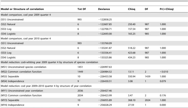
The main purpose of the tests was to investigate for each species and year which of the size correlations models that could be rejected or not (Hypothesis H01 and the models SS2, SS3 or SS4). It was especially important to establish whether the free unconstrained model could be reduced to a structured model so that abundance predictions could be made using a model with few parameters. All models were parameterised from the same correlation function (Eq. 5) on the transformed scale. The spatial correlation parameter was first tested for independence of size and time for each species and both years, and it was found that it was possible to distinguish between the space and size-time correlation. The Chi-Square likelihood ratio tests of the different models SS1. SS2, SS3, and SS4 (Table 2 and Table S1 in File S1) did not have sufficient power to reject any of the correlation structures for both cod and whiting in 2009 and 2010 because of the very high number of degrees of freedom in the main model. This indicates that there is no significant difference between (SS1) and (SS2, SS3, and SS4) with respect to the description of the correlation between size groups for cod any of the years (Table 2), and consequently we cannot reject a structured correlation model (hypothesis H01).
Higher power of the tests can be obtained by re-binning the data to 2-cm size groups and re-fitting the models (SS1)–(SS4), as this will very much reduce the degrees of freedom of model (SS1). When using 2-cm size groups, the test results for cod in both 2009 and 2010 (not shown) came out in favour of the log- and logistic transformations parameterising a structured size correlation
model, as the identity transform was rejected (pv0:02). Thus,
the identity transformation was excluded from the analysis. There is a trade-off between precision in the model by using 2-cm size groups compared with the high resolution in the rate of change in distribution when using 1-cm groups. In the present approach, we use the 1-cm groups to retain as much information as possible in the distribution dynamics of the fish. On average, a juvenile Baltic cod grows 1 cm in 6 weeks, and when using 2-cm size groups, the time resolution of 1.5 months is considered too high.
Consequently, a size-structured model cannot be rejected for any of the species for both years. In the multi-species and -year model extensions, the log transformation parameterisation was chosen because it is simpler than the logistic transformation in the sense that it does not contain any further parameters.
An alternative criterion for model selection is parameter consistency over time. In this case, the question regarding the four independent analysis (Figs. 2, 3, S2, S3) is which one of the transformation functions for the structured size correlation models (SS2)-(SS3) will have the most robust parameter estimates. In other words, are the images Figure 2c and Figure 3c (or 2d or 3d) for cod significantly different? Likewise, is this the case for Figure S2c and Figure S3c (or S2d and S3d) for whiting? Parameter estimates related to the logistic (d) and log (c) transforms display equal consistency over time, and here we have reported the results of the log-transform (c) (Table 3). All correlation parameters (a,b,c) (Eq. 1) related to size can be tested independent of the year effect, and, furthermore, the spatial correlation parameterdappears indepen-dent of both year and species (Table 3). It is remarkable that the
Figure 3. Model comparison for cod year 2010 quarter 4.SS1, unconstrained (a); SS2, natural scale (b); SS3, log scaled (c); SS4, logistic scaled (d).
parameterbdescribing the angular velocity of the oscillating part (Eq. 5) of the size-correlation is significantly different for cod and whiting, explaining the main differences in the species specific size correlation functions (Fig. 4). This result basically indicates that small and large cod occur in the same spatial regions, whereas this is not the case for whiting. This pattern is also visible from the initial analyses with animations of cod and whiting abundance patterns across size-groups from the surveys as described in Supporting Information Appendix A, i.e., where the whiting is observed more westerly as smaller individuals and more easterly as larger fish, whereas small cod are observed more easterly both for the very small and very large size classes. Consequently, there is a rather consistent structure in the size correlation within the species over time.
2. Multispecies models including species correlation The next step is to use the model to assess the possible correlation between species to test hypothesis H02. This is accomplished by comparing the four multispecies correlation models MS1–MS4 and testing whether the free, unconstrained species-size model MS1 can be reduced to the sub-models M2– MS4.
The combined analyses with the multi-species extension of the model considering species correlation involved runs under the log-transformed size for both species (Figs. 5, 2009 and S4, 2010). The results are presented in Figure 5 for 2009 and Figure S4 for 2010 and are covered in detail in the panel (a) that presents an image of the combined correlation of cod (the large square block) and whiting (the smaller square block) using the previous (separate) analysis for each species combined with the assumption of unconstrained species-size correlation between the two species. The next panel (b) is visually very similar to panel (a) and
represents the model reduction where cod and whiting are assumed to have a common correlation function. Despite the visual similarity between panel (a) and (b), the likelihood ratio test strongly rejects this reduction (Table 2). Panel (c) is an image of the
Table 2.Model comparisons with unconstrained size correlation versus natural, log and logistic scaled and model reductions
according to either species or year.
Model or Structure of correlation Tot Df Deviance Chisq Df Pr(.Chisq)
Model comparison, cod year 2009 quarter 4
(SS1) Unconstrained 993 2122858.25
(SS2) Natural 6 2122607.85 250.40 987 1.000
(SS3) Log 6 2122700.71 157.54 987 1.000
(SS4) Logistic 8 2122693.00 165.25 985 1.000
Model comparison, cod year 2010 quarter 4
(SS1) Unconstrained 993 2133760.09
(SS2) Natural 6 2133241.87 518.22 987 1.000
(SS3) Log 6 2133336.41 423.68 987 1.000
(SS4) Logistic 8 2133325.86 434.23 985 1.000
Model reduction: cod+whiting year 2009 quarter 4 by structure of species correlation
(MS1) Unconstrained species correlation 1451 2226997.63
(MS2) Common correlation function 1449 2226984.52 13.11 2 ,0.010
(MS3) Separable 10 2226433.58 550.94 1439 1.000
(MS4) Independence 9 2226430.51 3.08 1 0.079
Model reduction: cod year 2009+2010 quarter 4 by structure of year correlation
(MY1) Unconstrained year correlation 2036 2256427.46
(MY2) Common correlation function 2034 2256423.99 3.47 2 0.176
(MY3) Separable 10 2256055.89 368.10 2024 1.000
(MY4) Independence 9 2256028.29 27.59 1 0.000
doi:10.1371/journal.pone.0099151.t002
separable model reduction, and this model does not fit very well. Finally, panel (d) shows the model fit, assuming species indepen-dence. The likelihood ratio tests for (c) and (d) indicate that it is not possible to distinguish between (b), (c) and (d). In summary, none of the model reductions are valid because of the rejection of model (b) because of the combined nested structure of the test procedure. Consequently, (a) will have to be chosen as final model in this case, i.e., no constraints in the species correlation. The conclu are the same for cod and whiting in 2010 (Fig. S4), except that here the separable model visually appears to perform better than for 2009, and the species correlation is significantly non-zero. Below, we return to the overall conclusions on species correlation.
3. Multiyear analyses including year correlation
In MY1–MY4, the cod-whiting species correlation has been replaced by the corresponding 2009–2010 year correlation to test hypothesis H03. For both species (cod 2009 and 2010 in Fig. 6, and whiting 2009 and 2010 in Fig. S5), the common correlation function hypothesis in (b) cannot be rejected as p&0:18 and
p&0:05, for cod and whiting, respectively (Table 2 and Table S1 in File S1). Furthermore, the separable model (c) cannot be rejected, but the independence test (d) is rejected for both species. Consequently, for both species, one will select model (c), i.e., a separable correlation model, as the final model.
4. Summary of the results
Three main conclusions can be drawn. i) For the single species models, the size correlation models parameterised on natural (SS2), log (SS3) and logistic scale (SS4) cannot be rejected compared with the unconstrained model (SS1). ii) The uncon-strained species and year correlation models MS and MY 1–3 are all generalizations of the single species models SS 1–4. iii) Both multispecies and multiyear correlations (unconstrained) appear to occur (see Figures 5, 6, S4, S5 panels (a) and (b)). For the multiyear correlation models, it was possible to obtain a parameterised year correlation model, the separable model MY3, which was not
rejected, and this indicates that Hypothesis H03 can be accepted. In contrast, we cannot reject that species correlation occurs (hypothesis H02), but this correlation is very complex and resisted the parameterisation described here. The current models appear to perform better when describing time correlation than species correlation. A free, unconstrained species-size correlation model with many parameters is therefore still needed for describing the correlation between species.
5. Predicting abundance surfaces
The potential of the correlation model to make abundance surface predictions was analysed, first using (unconstrained) species correlation models (Figs. 7 and S6) and second using time correlation models (Figs. 8 and S7). An extended species or time correlation structure is useful to predict abundance surfaces of a target species when using only indirect data, i.e., data of the other species at the same yearorthe same species the year before. For all figures, the left panels represent the ‘‘observed’’ patterns (single species model predictions), and the right panels represent the corresponding predicted panels. The visual inspection reveals that of the performance of all predictions, the species-based predictions are perhaps the most accurate. These findings also support that we cannot reject hypothesis H02 when using a much more complex model in this comparison, i.e., the unconstrained species correlation model with many parameters, to perform the species-based predictions.
Discussion
1. Trawl survey analysis model development and general application
A length-based stochastic model of single-species stock dynamics including densities [6] was applied to the Baltic cod species based exclusively on survey data; however, this model was not spatially explicit. In the present study, an extension of the statistical LGCP model [3] is applied to the standard and extended BITS data for Baltic cod and whiting to investigate not only intraspecific size correlations, including spatial and temporal distribution patterns, but also potential interspecific correlation between species in relative density according to space, size, and time.
The motivation for developing size-based density models including species, time and spatial correlation is based on the apparent visual relationship between species from sequential abundance maps (as for instance presented in Figures 7, 8, S6, S7, first column, illustrating the spatial distribution by species by size group as well as described in Supporting Information Appendix A). Quantification and modelling of the covariance functions is performed either for the same species at different time periods or for different species at the same time. The aim is to empower spatial predictions of relative density of fish within and across species after constructing spatial abundance models that support hypotheses testing regarding alternative model specifica-tions. Such species/size time/size correlation models are high dimensional, and model reduction is sought to apply the models for predictions. We formulated natural model reduction hypoth-eses based on a size transformation that results in fish being able to be compared on a size scale.
2. Structure of size correlation models by species and size transformations used for model parameterisation
The separate single species analyses assumed that the spatial and the size correlations in density are independent among species. The analyses further revealed that the idea that fish can be compared on a size scale by transformations of the natural size
Table 3.Summary of single species runs: Parameter
estimates of log-transform model and size-correlation (first 5 parameters) plus spatial covariance parameters (final 9).
Estimate Std. Error
acod 2.42 0.26
awhi 0.98 0.11
bcod 1.19 0.16
bwhi 0.35 0.09
c 0.98 0.26
logd 27.02 0.57
logscod2009
1 0.61 0.06
logscod2010
1 0.37 0.08
logswhi2009
1 0.53 0.08
logswhi2010
1 0.24 0.12
logscod2009
2 20.47 0.14
logscod2010
2 20.05 0.11
logswhi2009
2 0.31 0.09
logswhi2010
2 0.29 0.09
scale cannot be rejected for any of the species for both years, and there is a rather consistent structure in the size correlation within species over time. The log and logistic size transformations, but not the natural (no transformation) for cod, were not rejected when changing the bins to 2-cm length groups. On this basis, hypothesis H01 cannot be rejected. As such, the model enables prediction, interpolation and animation of unobserved relative distribution and density patterns at any location and season of the year in the area for, e.g., cod and whiting.
3. Multi-species and multi-year correlation models according to model complexity
Regarding model complexity, the following conclusions have been drawn. For the relation between a year and the subsequent year of the spatial distribution of a given species/size, the simple reduced low dimensional model is adequate to describe the complicated observed correlation patterns, and a significant correlation between years was found. For the multispecies relationship, the simple structured models developed are not adequate to describe the correlation pattern, and thus, we were not able to decide if a significant species correlation exists. This indicates that the separable model is found too simple to describe the potential species/size correlation. However, it is remarkable how well the (unconstrained) species correlations model can predict a ‘‘missing’’ species, which indicates that species correla-tion may exist, and we cannot reject hypothesis H02. In general, the strength in the approach lies in the detailed description and
testing of the combination of species-size and time-size correla-tions.
For the single species models, area and time spatial variations in log fish density,gðs,xÞ, of a point in the space,x, for a given size are assumed random by nature. However, if some structure in relative fish densities according to animal behaviour exists, we expect to observe fish of similar sizes occupying the same spatial areas. For the two competing species, cod and whiting, we expect that fish of similar sizes of occupy the same spatial areas (sharing the same habitats, food sources, etc.) or fish of different sizes occupy the same spatial areas (due to predation on each other and even potential cannibalism). Both cod and whiting have, for the North Sea, been demonstrated to be competing species for the same habitats and to predate on each other (e.g., [13]). Interspecific relationships may play a role in the distribution patterns of WBC cod and whiting, but this phenomenon is not well understood [27,28,29,19]. There is spatial and temporal variation in biological interactions due to predation by cod in the Baltic Sea, where also cannibalism has been documented as an impacting factor in certain periods [30,31,20,12,32]. The levels of cannibal-ism are dependent on the abundance of juveniles and larger cod predators, their overlap in distribution, and the availability of alternative prey items for larger cod, such as sprat and herring [33,34,20,32]. In the WBS, there are also abundant competing gadoid predators in the form of whiting [12].
The basic single species model used (Eq. 1) includes three processes: large spatial scale variations for each size group,
small-Figure 5. Multispecies models for cod and whiting year 2009 quarter 4.MS1, unconstrained species correlation with separate parametric size correlation for each species (a); MS2, unconstrained species correlation with common parametric size correlation for both species (b); MS3, separable species-size correlation (c); MS4, no species correlation (d).
scale variations and a spatial/size correlation component describ-ing the spatial landscape by size. The large-scale variation is chosen as generally as possible, i.e., an unconstrained model including a parameter for each size group. The small-scale variation and correlation are assumed to be the same for each point in the space and depends only on the size correlation. The spatial/size correlation was modelled using a Gaussian random field, for which all possible ways between two spatial points are evaluated and for which shorter paths are preferred to longer paths. This model has the advantage that paths crossing land can be avoided.
For the multispecies models including species correlation, it was assumed that the parameters affecting the degree of spatial correlation are assumed to be the same for the species considered. This may be incorrect for species with different spatial behaviour. Similarly, for the multiyear analyses, it was assumed that these parameters are the same for the time periods considered.
Whether all of these assumptions are too restrictive or not depends on the species and time periods considered and must be tested statistically in each case. The results indicate all single species models and assumptions for cod and whiting in the WBS are not rejected. The same applies to the multiyear analyses, whereas the multispecies structured models are rejected.
It should be noted that estimation of spatially aggregated absolute abundance demands correction for bias in the log-normal distribution, especially if data are far from Gaussian. However, for
constant variance fields, the correction has no effect on relative abundance as used here. Estimation of absolute abundance is usually performed by posterior simulation as demonstrated by, e.g., Lewy and Kristensen [2]. The present paper does not include this problem because we consider all mean value parameters, mð Þsi , as nuisance parameters where we operate with relative abundance surfaces rather than simulating and predicting absolute abundance.
4. Further extension of the correlation structures and future studies
In the present analyses, we assume that there is no difference in the small- and large-scale size correlations [3]. In addition, we assume that the small-scale variations,eðs,xÞ, i.e., the within haul variations, are correlated across size-classes because of possible size-dependent schooling [3]. As small-scale variations can potentially be dominating, future studies should analyse differences in the large scale and small scale variation in relation to species, and an improved model should take into account differences between large-scale and small-scale variation.
For the multi-species extension, a structured size correlation model is used where correlations between size classes only depend on the distance between transformed sizes and where a common parameterisation on the different size transformation scales are applied (involving log transformed size) for both species. The same function for distance between transformed sizes does not
Figure 6. Multiyear models for cod year 2009 and 2010 quarter 4.Unconstrained year correlation with separate parametric size correlation for each year (MY1, a), Unconstrained year correlation with common parametric size correlation for both years (MY2, b), separable year-size correlation (MY3, c), No year correlation (independence) (MY4, c).
necessarily need to be used for both species. Figure 4 indicates that the parameter b, which describes the angular velocity of the oscillating part of the size-correlation, is significantly different for cod and whiting, explaining the main differences in the species specific size correlation functions when applying the same size correlation structure (i.e., the same size class transformation). Higher correlation between species might have been achieved by applying different functions according to distance in transformed size where more complex species specific structures are taken into account. Future studies should investigate further alternative species specific functions for transformation of size to parameterise the same size correlation model.
The present analyses have only covered model development and data analysis of observations from relatively few years, quarters and species. Further studies should investigate the structure of the correlation models and their size transformation
parameterisations as well as the multi-species correlation models for an extended set of years, quarters and fish species.
The purpose of our study was to establish a correlation structure describing the spatial distribution and relative density patterns of a single species of all size-classes for a time-snapshot(1 month). Our modelling of animal density is based on considerations and testing of the processes acting on a spatial scale using survey catch rates by size group by haul. Alternatively, future studies could consider combining the existing area-based time snapshot models with new models tracking the movements in time. Perhaps such models modelling the correlation between the directional movements could better capture the fish behaviour and the resulting spatial fish distribution.
Finally, model-based geostatistical methods can be further applied to investigate optimal survey designs for different species
Figure 7. Maps of relative whiting abundance 2009/Q4based on whiting observations(left column) versus the same mapsbased on cod observations(right column) utilizing MS1 model of Table 2.The three row panels indicate three whiting size groups in cm.
and size groups using the extended BITS survey dataset established here.
Supporting Information
Figure S1 Spatial correlation measured from given
centre point. It shows the properties of the Gaussian Markov Random field co-variance (Q21) generated from Eq. 4, which indicates a decreasing correlation according to distance taking into to account the geometry of the grid. The co-variance (correlation) depends on all possible ways between two points, i.e., it is an integral over all possible ways between the centre point and any other point weighted with the distance of the way (in the sea and not over land).
(TIF)
Figure S2 Model comparison for whiting year 2009
quarter 4.SS1, unconstrained (a); SS2, natural scale (c); SS3, log scale (d); SS4, logistic scaled (d).
(EPS)
Figure S3 Model comparison for whiting year 2010
quarter 4.SS1, unconstrained (a); SS2, natural scale (b); SS3, log scaled (c); SS4, logistic scaled (d).
(EPS)
Figure S4 Multispecies models for cod and whiting year 2010, quarter 4.See figure explanation for Figure 5.
(EPS)
Figure S5 Multiyear models for whiting year 2009 and 2010 quarter 4.See figure explanation for Figure 6.
(EPS)
Figure 8. Predictive power of the models illustrated by maps of relative cod abundance 2010/Quarter 4 based oncod observations that year(left column) versus the same maps based oncod observations previous year(right column) utilizing model MY3.The three row panels indicate three cod size groups in cm.
Figure S6 Maps of relative whiting abundance 2010/Q4 based on whiting observations(left column) versus the same maps based on cod observations (right column) utilizing MS1 model of Table S1 in File S1.The three row panels indicate three whiting size groups in cm.
(EPS)
Figure S7 Predictive power of the models illustrated by maps of relative whiting abundance 2010/Quarter 4 based on whiting observations that year (left column) versus the same maps based on whiting observations previous year (right column) utilizing model MY3.The three row panels indicate three whiting size groups in cm. (EPS)
File S1 Table S1, (containing model comparisons with unconstrained size correlation versus natural, log and logistic scaled, and model reductions according to either species or year for whiting year 2009 quarter 4, whiting quarter 4 2010, cod+whiting year 2010 quarter 4, and whiting year 2009+2010). Keywords; Appendix A (with description of specific distribution patterns for cod and whiting for different size groups); Appendix B (with description of methods
on (B1) how to parameterise a general positive definite (PD) correlation matrix w? R?, (B2) how to parameterise a general positive definite correlation matrix with given marginal, and (B3) the proof for this).
(DOC)
Acknowledgments
We would like to thank our colleagues in the International Fehmarn Belt Science Provision Project (Femern Bælt A/S, DK), in the IMAGE (MAFIA) Danish Strategic Research Council Project, and the EU FP7 SOCIOEC Project for their scientific contributions to the present publication that made it possible.
Author Contributions
Conceived and designed the experiments: JRN. Performed the experi-ments: JRN. Analyzed the data: JRN KKR PL FBA. Contributed reagents/materials/analysis tools: JRN KKR PL FBA. Wrote the paper: JRN KKR PL. Revising the manuscript critically for important intellectual content: JRN KKR PL FBA. Interpretation of the data: JRN KKR PL FBA. Final approval of the version to be published: JRN KKR.
References
1. Kristensen K (2009) Statistical aspects of heterogeneous population dynamics. PhD Thesis Department of Mathematical Science University of Copenhagen. 2. Lewy P, Kristensen K (2009) Modeling the distribution of fish accounting for
spatial correlation and overdispersion. Can J Fish Aquat Sci 66: 1809–1820. 3. Kristensen K, Thygesen UH, Andersen KH, Beyer JE (2014) Estimating
spatial-temporal dynamics of size structured populations. Can J Fish Aquat Sci 71(2) 326–336. E-Pub 13 November 2013. doi:10.1139/cjfas-2013-0151.
4. Stefa´nsson G (1996) Analysis of groundfish survey abundance data: combining the GLM and delta approaches. ICES J Mar Sci 53(3): 577–588. doi:10.1006/ jmsc.1996.0079
5. O’Neill MF, Faddy MJ (2003) Use of binary and truncated negative binomial modelling in the analysis of recreational catch data. Fish Res 60(2–3): 471–477. doi:10.1016/S0165-7836(02)00101-7
6. Kristensen K, Lewy P, Beyer JE (2006) How to validate a length-based model og single-species fish stock dynamics. Can J Fish Aquat Sci 63(11): 2531–2542. doi:10.1139/F06-135
7. Hrafnkelsson B, Stefa´nsson G (2004) A model for categorical length data from groundfish surveys. Can J Fish Aquat Sci 61(7): 1135–1142. doi:10.1139/f04-049
8. Rivoirard J, Simmonds J, Foote KG, Fernandes P, Bez N (2000) Geostatistics for estimating fish abundance. Blackwell Science Oxord UK.
9. Stelzenmu¨ller V, Ehrich S, Zauke GP (2005) Effects of survey scale and water depth on the assessment of spatial distribution patterns of selected fish in the northern North Sea showing different levels of aggregation. Mar Biol Res 1(6): 375–387. doi:10.1080/17451000500361009
10. Diggle PJ, Tawn JA (1998) Model-based geostatistics. Appl Statist 47(3): 299– 350.
11. Jansen T, Kristensen K, Payne M, Edwards M, Schrum C, et al (2012) Long-term retrospective analysis of mackerel spawning in the North Sea: a new time series and modeling approach to CPR data. PLoS ONE 7: e38758. doi:10.1371/ journal.pone.0038758
12. ICES (2012a) Report of the Baltic Fisheries Assessment Working Group 2012. ICES WGBFAS Report 2012 ICES CM 2012/ACOM:10.
13. Bromley P J, Watson T, Hislop JRG (1997) Diel feeding patterns and the development of food webs in pelagic 0-group cod (Gadus morhuaL.), haddock (Melanogrammus aeglefinusL.), whiting (Merlangius merlangusL.), saithe (Pollachius virensL.), and Norway pout (Trisopterus esmarkiiNilsson) in the northern North Sea. ICES J Mar Sci 54: 846–853.
14. Nielsen JR, Limborg M (2009) Managing fleets and fisheries rather than single stocks – conceptual change in European fisheries management advice. World Fishing 58 (1): 8–9.
15. Marchal P, Nielsen JR, Hovga˚rd H, Lassen H (2001) Time changes in fishing power in Danish cod fisheries of the Baltic Sea. ICES J Mar Sci 58: 298–310. 16. Bastardie F, Nielsen JR, Kraus G (2010a) The eastern Baltic cod fishery: a fleet-based management strategy evaluation framework to assess the cod recovery plan of 2008. ICES J Mar Sci 67: 71–86.
17. Bastardie F, Vinther M, Nielsen JR, Ulrich C, Storr-Paulsen M (2010b) Stock-based vs. fleet-Stock-based evaluation of the multi-annual management plan for the cod stocks in the Baltic Sea. Fish Res 101: 188–202. doi:10.1016/j.fish-res.2009.10.009
18. Bastardie F, Nielsen JR, Miethe T (2013) DISPLACE: a dynamic, individual-based model for spatial fishing planning and effort displacement - integrating underlying fish population models. Can J Fish Aquat Sci 71: 1–21. doi: 10.1139/ cjfas-2013-0126
19. EU STECF (2012) Multi-Species Management Plans for the Baltic. EU-EWG-12-02 Rostock (D) March 2012 STECF 12-06 Report March 2012 Luxembourg: Publications Office of the European Union, 2012. ISSN 1831-9424 (print). (Eds. Simmonds and Jardim). (Co-reporting with ICES WKMultBalt 2012).
20. Neuenfeldt S, Ko¨ster FW (2000) Trophodynamic control on recruitment success in Baltic cod: the influence of cannibalism. ICES J Mar Sci 57: 300–309. 21. ICES (2012b) Report of the Baltic International Fish Survey Working Group.
ICES WGBIFS Report 2012: ICES CM 2012/SSGESST:02. (Including Addendum 1: Manual for the Baltic International Trawl Surveys (BITS Manual) and Addendum 2: Manual for International Baltic Acoustic Surveys (IBAS)).
22. Nielsen JR, Hansen UJ, Ernst P, Oberst R, Rehme W, et al (2001) Final and consolidated report of the EU Study Project No. 98/099 ISDBITS: Improve-ment of stock assessImprove-ment and data collection by continuation, standardisation and design improvement of the Baltic International Bottom Trawl Surveys for fishery resource management. Rep. DG FISH A4/JF 2001. European Commission Brussels: 143 pp+VI+10 Annexes (349 pp.).
23. Lewy P, Nielsen JR, Hovga˚rd H (2004) Survey gear calibration independent of spatial fish distribution. Can J Fish Aquat Sci 61: 636–647.
24. Enga˚s A, Godø OR (1989) Escape of fish under the fishing line of a Norwegian sampling trawl and its influence on survey results. ICES J Mar Sci 45: 269–276. 25. Cressie N (1993) Statistics for spatial data. New York: Wiley.
26. Rue H, Held L (2005) Gaussian Markov Random Fields. Chapmann & Hall/ CRC Boca Raton.
27. Nielsen JR, Lundgren B (1999) Hydroacoustic ex-situ target strength measurements on juvenile cod (Gadus morhua L.). ICES J Mar Sci 56: 627–639. 28. Nilsson LAF, Høgsbro U, Lundgren B, Nielsen BF, Nielsen JR, et al (2003) Vertical migration and dispersion of Sprat (Sprattus sprattus) and herring (Clupea harengus) schools at dusk in the Baltic Sea. Aquat Liv Res 16: 8 pp.
29. Lundgren B, Nielsen JR (2008) A method for the possible species discrimination of juvenile gadoids by broad-bandwith backscattering spectra vs. angle of incidence. ICES J Mar Sci 65: 581–593.
30. Sparholt H (1994) Fish species interactions in the Baltic Sea. Dana 10: 131–162. 31. Uzars D, Plikshs M (2000) Cod (Gadus morhuaL.) cannibalism in the central Baltic: interannual variability and influence of recruit abundance and distribution. ICES J MarSci 57: 324–329.
32. Eero M, Vinther M, Haslob H, Huwer B, Casini M, et al (2012) Spatial Management of marine resources can enhance the recovery of predators and avoid local depletion of forage fish. Cons Letters 0: 1–7.
33. Ko¨ster FW, Mo¨llmann C, Neuenfeldt S, St John MA, Plikshs M, et al (2001a) Developing Baltic cod recruitment models. I. Resolving spatial and temporal dynamics of spawning stock and recruitment for cod, herring and sprat. Can J Fish Aquat Sci 58: 1516–1533.