of Chemical
Engineering
ISSN 0104-6632 Printed in Brazil www.scielo.br/bjce
Vol. 35, No. 02, pp. 745 - 756, April - June, 2018 dx.doi.org/10.1590/0104-6632.20180352s20150727
SOFT SENSOR MODELS FOR A FRACTIONATION
REFORMATE PLANT USING SMALL AND
BOOTSTRAPPED DATA SETS
Željka Ujević Andrijić
1*, Matija Cvetnić
2and Nenad Bolf
11 Department of Measurement and Process Control, Faculty of Chemical Engineering and Technology,
University of Zagreb, Savska c. 16/5A, 10000 Zagreb, Croatia, Phone: + (385) (1) 4597-150 E-mail: [email protected]; E-mail: [email protected]
2 Department of Analytical Chemistry, Faculty of Chemical Engineering and Technology, University of
Zagreb, Marulićev trg 20, 10000 Zagreb, Croatia, Phone: + (385) (1) 4597-205 E-mail: [email protected]
(Submitted: November 9, 2015; Revised: November 2, 2016; Accepted: January 3, 2017)
Abstract - In refinery plants key process variables, like contents of process stream and various fuel properties, need to be continuously monitored using adequate on-line measuring devices. Such measuring devices are often unavailable or malfunction and, hence, laboratory assays which are irregular and time consuming and therefore not suitable for process control are inevitable alternatives. This research shows a comparison of different soft sensor models developed from a small industrial data set with soft sensor models developed from data generated by a bootstrap resampling method. Soft sensors were developed applying multiple linear regression, multivariable adaptive regression splines (MARSpline) and neural networks. The purpose of the developed soft sensors is the
assessing of benzene content in light reformate of a fractionation reformate plant. The best results were obtained
by the neural network-based model developed on bootstrapped data.
Keywords:Bootstrap, neural network, multivariable adaptive regression splines, soft sensor, process modeling.
INTRODUCTION
Due to growing demands for better product quality but lower product prices and strict safety
and environmental rules, there is a need for optimal
control of chemical processes. Process control is based
on continuously measured process variables in order
to get satisfactory product quality with minimum consumption of raw materials and energy. Many of
the key process variables which determine product
quality in the chemical, petrochemical and oil industry
are difficult or even not possible to be continuously measured. With the process knowledge and a lot of easy measurable process variables it is possible to link the secondary, easily measured variables (like the
flow, pressure, temperature and level) with variables
that are not possible to be continuously measured, the
so-called primary variables.
On-line process analyzers are often not available on grounds of malfunction (due to harsh process conditions), during regular maintenance and frequent need for calibration. This problem can be solved by soft sensors application (Zamprogna et al., 2004;
Qin, 2007). Soft sensors can work in parallel with analyzers and measuring devices, allowing fault
detection schemes.
For the reason of the uncertainty and complexity of industrial processes, fundamental models are often
unavailable or inadequate. In industrial plants large
quantities of process data are measured and stored
in historical data bases which enable identification of data driven models (Fortuna et al., 2007).
In the present study, soft sensors for the prediction of benzene content in the fractionation reformate
plant are developed and analyzed. Two linear multiple models, two models of multivariable adaptive regression splines (MARSpline) and two neural network models are developed. Within these models, one model is developed using a small experimental data set, while the other model is developed using
bootstrap generated data.
DATA PREPROCESSING
Selection of the representative process data requires
the cooperation of the designer of the soft sensor and plant experts, operators in the control room and process engineers. It is necessary to detect missing data and to
remove unwanted components such as outliers, offset,
trend and noise.
Since that process analyzers are often inaccessible,
the key process properties must be determined by rare
and time-consuming laboratory analysis. In such cases,
a small number of data is available, so it is necessary
to collect as much data as possible during regular
operation of the plant. When developing the model
with a small number of data there is a strong possibility
of poor generalization because the developed model does not take into account process dynamics and all process regimes (Fortuna et al., 2007).
To avoid problems of a small data set several strategies have been considered in the literature. Most of them are based on injecting noise into the available
data or by using the bootstrap resampling approach
(Napoli and Xibilia, 2011). There is also a method
based on an aggregation of neural models, trained on
different training data sets, which are obtained by noise injection and bootstrap resampling (Lanuette et al.,
1997; Tsai and Der-Chiang, 2008). Injecting noise into the training set means adding zero-mean fixed-variance
Gaussian noise, or adding zero-mean Gaussian noise
variable variance according to the signal amplitude.
Application of ensemble learning algorithms for the
improvement of prediction performance of the system
can also be found in Caruana et al. (2000), Polikar
(2006) and Polikar (2012). Li et al. (2013) applied injection of Gauss noise to the ensemble of the Least
Square Support Vector Machine (LS-SVM) model. Data set diversity can be increased by integration of
all mentioned techniques, i.e., bootstrap method, noise
injection method and stacked neural networks (Di
Bella et al., 2007).
Some other models dealing with the small data set
problem are presented in literature, like Zhou et al.
(2012) who developed a bootstrap aggregated Partial
Least Square regression model. Li et al. (2013) applied injection of Gauss noise to the ensemble of the Least
Square Support Vector Machine (LS-SVM) model. A somewhat different approach which deals with dynamic behaviour is considered by Zhu et al. (2009)
where an output error method for the identification
of a dual fast rate model directly from fast input and slow output data is proposed. A similar approach dealing with dual-rate systems is presented by Ding
and Chen (2004), who applied FIR models to predict
unmeasurable noise-free outputs, and identify the parameters of underlying fast single-rate models.
In this paper, the bootstrap method is applied with
a view to increase training data set diversity and to improve the generalization capabilities of the neural network.
Bootstrap method of generated additional data
The bootstrap method is a general resampling procedure for estimating the statistical distribution
on independent observations introduced in Efron (1979). If
there is a function of distribution, F, with independent
variables, x1, x2,… xn, there is a need to investigate
the sampling distribution and variability of a function
calculated from a sample of size n.
The idea of the nonparametric bootstrap method
is to simulate data from a cumulative distribution
function, Fn. Fn is a discrete probability distribution
which gives probability 1/n for every observed value
of x1, x2, ..., xn. A sample of size n of a function Fn is a sample of size n drawn with replacement from a set of x1, x2, ... , xn. In case of a large sample size, n, calculating
the distribution is very complicated and therefore it is
recommended to create a bootstrap distribution from simple random sampling with replacement.
The basic steps of the bootstrap procedure are
(Efron and Tibshirani, 1993):
1. Construction of an empirical probability distribution, Fn, from samples by placing a probability of 1/n for each case, x1, x2, ..., xn of the sample. This is the empirical distribution function of the samples, which is the
nonparametric maximum likelihood estimate
of the population distribution, F.
3. Calculating some statistical parameter, Tn of a resampled sample.
4. Repeating steps 2 and 3, B number of times, where B is a large number, in order to create B resamples. Typically, B is at least equal to 1000
when an estimate of the confidence interval
around Tn is required.
5. Construction of the relative frequency histogram from the B number of Tn by placing a probability of 1/B for each case. The distribution obtained is the bootstrapped estimate of the sampling distribution of Tn.
SOFT SENSOR MODELS
In the case of long output delays, static models are
usually developed. In many industrial processes, where
nonlinearity is slightly present and processes are almost
steady- state, linear static process can be identified. In processes where defined or undefined nonlinearities are significantly present, nonlinear models must be applied and the identification procedure thus becomes more complex (Fortuna et al., 2007).
Linear multiple model
The general equation of linear multiple models
is presented in Equation (1) where parameters bi of each input Ui are analogue to the slope, also called the
regression coefficients.
(1)
n is the number of input variables or predictors. MARSpline model
Multivariate Adaptive Regression Splines, or the
MARSpline technique has the purpose to predict
the value of a set of dependent variables from a set of independent or predictor variables (Friedman, 1991). MARSpline constructs a relationship between dependent and independent variables from a set of coefficients and basis functions that are entirely
determined from the data. MARSpline algorithm
operates like a multiple piecewise linear regression, where each breakpoint (estimated from the data) defines the "region of application" for a particular (simple)
linear equation. The MARSpline algorithm builds
models from two-sided truncated functions (t-x)+ i ( x-t)+ of the predictors (x) which serve as basis functions for a linear or nonlinear expansion that approximate the underlying function f(x). The parameter t is the
knot of the basis functions defining the "pieces" of the
piecewise linear regression. The "+" sign next to the
terms (t-x) and (x-t) denotes that only positive results
of the respective equations are considered; otherwise the respective functions evaluate to zero.
Basis functions are defined as:
(2)
Parameter t defines the “pieces” of the piecewise linear regression estimated from the data. The
MARSpline model for a dependent variable y, and M
terms can be summarized in the following equation:
(3)
where the summation is over the M terms in the model, and bo and bm are parameters of the model. Function H
is defined as:
(4)
where xv(k,m) is the predictor in the k'th of the m'th product. For the order of interactions K=1 the model is
additive, and for K=2 the model is pairwise interactive.
Neural network
The full data set was divided randomly into three subsets: the training subset, the testing subset (in order to prevent overfitting) and the validation subset. Weights of the neural network are continually
calculated using training data. At the end of each
iteration (iteration refers to each passage of all the data for learning through the network), the network predicts a set of values on the test data set. If the test set error is greater than the specified tolerance, the next
iteration will be carried out. The process is repeated
until the error is less than the specified tolerance, or the predefined number of iteration is reached. To evaluate the model results, a validation data set was used,
which is an independent data set that was not applied
in training. Multi-Layer Perceptron (MLP) is a typical neural network with a backpropagation algorithm
which contains of one input and one output layer, and
at least one hidden layer. While the network is in the process of learning, information is propagated back through the network, where the weights are corrected and updated (Nørgaard et al., 2000).
All developed models are evaluated by the
comparison of model performance with the
performance of the real process using the validation
data set within the considered process conditions. It is important to the test model on an independent real
y
b
b U
i i i n 0 1$
=
+
=/
(
x
t
)
x
t
x
t
otherwise
0
>
-
+=
G
-
J
( )
(
)
y
f x
mH
kmx
v k m( , )m M 0 1
b
b
=
=
+
=/
(
)
H
kmx
v k m( , )h
-data set (not used for model estimation) to approve
the model applicability and reliability. Validation data set common indicators of model performance are the
Pearson correlation coefficient (5) and coefficient of determination (6), defined by the following equations:
(5)
(6)
The adjusted coefficient of determination, based on the number of degrees of freedom, is given by:
(7)
Other popular criteria of numerical model
evaluation reported in practical examples are the root mean square error (8) and mean absolute error (9)
(8)
(9)
PROCESS DESCRIPTION
Catalytic reforming is one of the most important
processes in the oil industry where refinery crude oil
with low octane number in the presence of a catalyst
converts into a high octane reformate (Cerić, 2012).
Catalytic reformate, as one of the main gasoline
components, contains a very high concentration of environmentally undesirable benzene (5-6 vol. %). In
order to satisfy technical and legal norms regarding the benzene content in fuels, currently less than 1
vol. %, benzene needs to be removed from reformate. European emission standards (such as EURO IV and EURO V) for vehicle exhaust emission and MSAT (Mobile Source Air Toxics) regulations
limit the amount of benzene in gasoline, due to the
hazardous effect of benzene on health and its negative environmental impact. It is possible to control the
formation of benzene by prefractionation of gasoline and by adjustment of the end distillation point of
heavy gasoline or by increasing the end distillation
point of light gasoline. Unfortunately, it is not possible
(
) (
)
(
)(
)
R
y
y
y
y
y
y
y
y
i i i n i i i n 2 2 1 1
=
-
--
-= =z
{
z
z
/
/
(
)
,
.
R
y
y
y
y
R
0
1
i i n i i n 2 1 2 1 2 2#
#
=
-== @ C
z
/
/
(
)
(
)
R
n
K
n
R
1
1
1
1
adj 2$
=
--
+
-
-(
)
RMS
n
y
iy
i i n 2 1=
-=z
/
e
MSEn
1
y
y
exp,i i n 1$
=
-=z
/
to completely prevent formation of benzene; therefore, the best solution is the removal of benzene compounds
from reformate by post fractionation in a splitter. Although benzene has a high octane number and
high calorific values, its content in light reformate needs to be reduced to 1%. This is due to the fact that
benzene is a precursor for the formation of cyclohexane in the process of isomerization, and thus an undesirable
component of gasoline (low octane number).
Fractionation of the reformate is used for the separation of light contents found in the reformate. Light reformate contains mostly C5 and C6 hydrocarbons, i.e., the fraction which contains pentane and C6 hydrocarbons with an end distillation point of around 85ºC at atmospheric pressure. The benzene-rich fraction, whose boiling point is between light and
heavy reformate, is separated from catalytic reformate.
The fractionation reformate plant with the
variables used for soft sensor development is given in
Figure 1. Reformate enters into column C-1 where the
light reformate is separated from the mixture of heavy
reformate and benzene fraction. The bottom product of column C-1 is the feed for the column C-2, where
the benzene fraction will be separated from the heavy
reformate.
In the laboratory the benzene content is determined and monitored in accordance with the standard EN
238:1996/A1:2003 Liquid petroleum products - Petrol
- Determination of the benzene content by infrared spectrometry.
MODEL DEVELOPMENT
In the refinery the continuous measurement of
benzene content in the reformate is crucial. A benzene on-line chromatographic analyzer is frequently under maintenance and sometimes faulty. Considering these facts soft sensors for the continuous on-line estimation
of benzene content in light reformate were developed. During the preliminary test ten input variables (temperatures, pressures and flows) that may affect
benzene content in light reformate are considered.
Sensitivity analysis, correlation analysis, PCA and
PLS methods were performed for the selection of
relevant model inputs.
Also, mutual correlations between inputs as well as
process engineer experience were taken into account during analysis (Ujević Andrijić et al., 2012).
The desired top product composition is determined
Figure 1. Reformate fractionation plant.
the entrance to the C-1 column (feed) can influence the whole temperature column profile and hence can also influence the product composition. The temperature column profile can also be affected by the outlet temperature of heater H-1 (cascade TC018-FC009) which finally has an influence on top product composition. Changes in the temperature profile in the column have an influence on column pressure (PI009).
PI009 and TC 003 are also indicators of possible
disturbances in the column (fluctuations in top column pressure, temperature or flow).
The following continuously measured variables were chosen as key input variables for particular soft sensor development:
- C1 inlet stream temperature, TC-001 (U1);
- C1 column bottom temperature (outlet from H-1), TC-018 (U2);
- C1 column temperature, TC-003 (U3);
- C1 column pressure, PI-009(U4) and
- Pump around flowrate, FC-002 (U5).
During the collecting of input and output data the
period with different process regime (various process
dynamics) is obtained to enable better training. Process
data was obtained from the plant history database
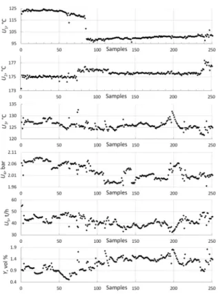
over a continuous period of three weeks, i.e., 6000 input data with sampling time of five minutes were collected. The model output variable was determined by laboratory measurement every two hours, thus 251
output data were obtained. The number of each input
data (sampled every five minutes) must correspond to the number of output data (sampled every two hours);
therefore, 251 data of each input and output were
synchronized (Figure 2).
Data preprocessing included detecting and
removal of outliers and data filtering (Ujević Andrijić
et al., 2012). The model development and the model
validation used 80% and 20 percent of the overall data set, respectively. By applying the bootstrap method,
Figure 2. Plot of inputs and output data.
Multiple linear models, MARSpline models and
models of MLP neural networks are developed in two ways:
• In the first case, the models were developed from a small data set, containing 201 measured data
of every real input and output, while the model is validated on the 50 remaining output data.
• In the second case, 6000 input data generated by the bootstrap method and 6000 generated
output data were taken for model development. The model estimation used 80% randomly chosen data, while 20%, i.e., 1200, remaining data were used for the model validation. Additional model validation was carried out on
251 laboratory measured output data.
Models were developed in software Statsoft Statistica version 12.5.
RESULTS AND DISCUSSION
Linear models
The linear model developed on small data set was presented with the following equation:
.
.
.
(10).
.
.
y
U
U
U
U
U
5 545
0 019
0 012
0 097
2 738
0 004
1 2
3 4 5
=-
-
+
+
-
+
Statistical parameters of the linear model are shown
in Table 1. Quite high values of correlation coefficients and small values of absolute and RMS errors indicate good model accuracy.
Table 1. Statistical parameters of the linear model (a small data set).
Parameter Estimation Validation
R 0.881 0.928
R2 0.777 0.862
Radj 0.772 0.859
eMSE, vol. % 0.094 0.071
RMS, vol. % 0.140 0.111
Figure 3 shows the graphical comparison between the model output and measured output data using the
validation data set. It can be noted that the model
output satisfactorily follows the changes in measured
output with some minor deviations.
Figure 3. A scatterplot of the linear model vs. validation experimental
data (a small data set).
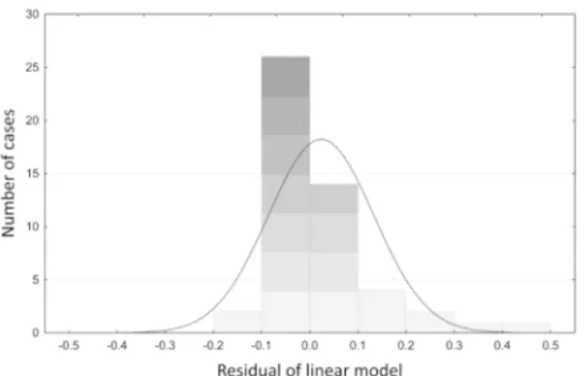
Figure 4 represents the histogram of linear
model residuals (differences between estimated and experimental outputs). Residuals are normally
distributed with a narrow bell shape, centered on zero. It can be seen that most of the errors lie between -0.1
and 0.1 vol. % benzene content, which leads to the
conclusion that the model satisfactorily matches with laboratory results.
The linear model was developed using 6.000 bootstrapped data (Equation 11).
(11)
Table 2 shows statistical parameters of the linear
model developed on the bootstrap expanded data and additionally validated on 251 real output data. From
the statistical indicators of model quality in Table 2
it can be concluded that the linear model developed
.
.
.
.
.
.
y
U
U
U
U
U
9 644
0 028
0 001
0 094
1 026
0 004
1 2
3 4 5
=-
-
-
+
on bootstrapped data shows somewhat poorer
performance than the previously mentioned linear
model. The same can be concluded from Figure 5 showing higher dissipation around the y = x direction.
Histograms of model residuals (Figure 6) show a
wider bell, i.e., the residuals are somewhat higher
than the linear model developed on small data. Even
though the statistical parameters of the linear model
developed on small data set are unexpectedly better, it is not the case with diversity in the results on different
data sets. Statistical parameters of the linear model
developed on bootstrapped data calculated on all three subsets are very similar, being a good indicator of model applicability to different data sets.
Figure 4. Distribution of the linear model residual on validation data (a
small data set).
Table 2. Statistical parameters of the linear model (generated data set).
Parameter Estimation Validation Real data
R 0.837 0.839 0.838
R2 0.700 0.704 0.702
Radj 0.700 0.704 0.701
eMSE, vol. % 0.119 0.119 0.119
RMS, vol. % 0.167 0.167 0.167
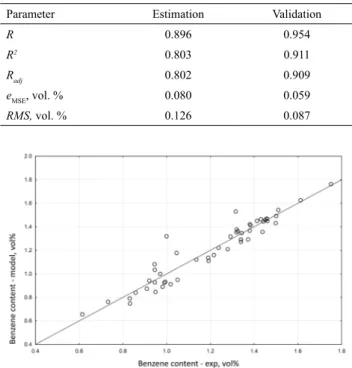
MARSpline models
Several MARSpline models with varying number
of basis functions and degrees of interaction using
small datasets were developed. The difference in the statistical indicators of these models was insignificant, so the parameters of the simplest developed model were chosen: eight basis functions, one degree of interaction
and acriterion penalty of two. In the case of the model
developed with bootstrapped data, the model with 13
basis functions, one degree of interaction and criterion penalty of two was selected. Statistical parameters of
the MARSpline model developed on the small data
set are reported in Table 3. From statistical model
Figure 5. A scatterplot of linear model vs. experimental validation data
(generated data set).
Figure 6. Distribution of linear model residuals on validation data
(generated data set).
properties, Figure 7 and Figure 8, good matching of
model output with experimental data can be observed.
Statistical parameters of the MARSpline model
developed using generated data are presented in Table 4. As in the case of the linear model developed on generated data, the MARSpline model achieved approximately same statistical values in all three
subsets, although somewhat better than the linear model. Very good matching of the MARSpline model
and experimental data on the validation data set can be
seen in Figures 9 and 10.
By comparing models having the same structure
types it can be concluded that linear and MARSpline
models developed on the generated bootstrapped data have greater ability for generalizations than models developed on small data sets. By comparing the linear
models with MARSpline models, it is clear that the
MARSpline models have a narrower distribution of
model residuals and better graphical comparison of model with experimental data. Statistical parameters of the MARSpline model are also better compared
Table 3. Statistical parameters of the MARSpline model (a small data set).
Parameter Estimation Validation
R 0.896 0.954
R2 0.803 0.911
Radj 0.802 0.909
eMSE, vol. % 0.080 0.059
RMS, vol. % 0.126 0.087
Figure 7. A scatterplot of the MARSpline vs. validation experimental data
(a small data set).
Figure 8. Distribution of MARSpline model residuals on validation data
(a small data set).
Table 4. Statistical parameters of MARSpline model (generated data set).
Parameter Estimation Validation Real data
R 0.915 0.918 0.915
R2 0.838 0.843 0.836
Radj 0.838 0.843 0.836
eMSE, vol. % 0.076 0.076 0.078
RMS, vol. % 0.113 0.112 0.115
Neural network models
The overall data set is randomly divided into three subsets: a training set which contains 60 % of the data, while the remaining 40 % of data are allocated to the testing (20%) and validation sets (20%). In
order to choose the optimal number of neurons in the
Figure 9. A scatterplot of MARSpline vs. validation experimental data
(generated data set).
Figure 10. Distribution of MARSpline model residuals on validation data
(generated data set).
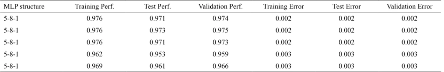
hidden layer and adequate transfer functions, the five best ones out of 1000 preliminary developed neural networks have been selected. The number of hidden neurons varied from 3 to 8. Exponential, sigmoid,
hyperbolic tangent and linear transfer function were
tried. In the development of neural network on the basis of the small data set (251 data), the bootstrap
subsampling method was used for the selection of learning data. The bootstrap method of subsampling randomly chooses data with a possibility of repeating
the same data (i.e., reusing them) an unlimited number
of times. It is common that the data set has the same size as the original data set, but with regard to the nature of a method, all data will not be selected. In the preliminary research, using the small data set, the
structure of a 5-3-1 network with hyperbolic tangent
transfer functions in the hidden layer was chosen. This
network contains five neurons in the input layer, three
in the hidden and one in the output layer.
In the MLP model developed on 6000 generated data, a 5-8-1structure of the network with logarithmic
Table 5. Selection of the best network developed on the small data set.
MLP structure Training Perf. Test Perf. Validation Perf. Training Error Test Error Validation Error
5-3-1 0.957 0.948 0.710 0.006 0.004 0.026
5-3-1 0.944 0.922 0.934 0.007 0.005 0.005
5-3-1 0.909 0.857 0.941 0.011 0.011 0.005
5-3-1 0.965 0.892 0.821 0.004 0.008 0.018
5-3-1 0.807 0.878 0.938 0.023 0.013 0.005
There are plenty of possible combinations of
the train-test-validation data set regarding random initialization of network weights and random
sampling of data to each subset. Therefore, with the
aim to improve generalization, 1000 networks of given topology were developed using the small data set, from which five best networks were selected (Table 5). Five best neural networks were chosen using statistical criteria like correlation coefficients and mean square errors of each subset and small diversity in errors of
each subset.
Using data generated by the bootstrap method,
1000 networks of given topology were developed from which the five best ones were selected and, among them, the best neural network was chosen, Table 6.
Statistical parameters of the neural network models developed on the small data set are shown in Table 7. High values of correlation coefficients and small errors point out that the model very well describes the actual data. Such good matching with minor deviations is also observed in Figures 11 and 12.
In Table 8 statistical parameters of the neural
network developed on the generated data set are presented. Improved statistical parameters with almost the same values for the estimation and validation
data sets show high model accuracy, which is better
than the MLP model developed on the small data set. From Figure 13, it can be seen that deviations from
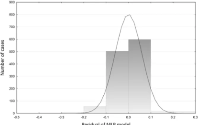
the direction y = x are minimal on the entire dataset. In Figure 14 for the histogram, it is clear that most of
the errors lie between -0.1 and +0.1 vol. % of benzene
content.
When all developed models are compared, it can be concluded that the best results are achieved by the neural network models developed on generated
Table 6. Selection of the best network developed on the generated data set.
MLP structure Training Perf. Test Perf. Validation Perf. Training Error Test Error Validation Error
5-8-1 0.976 0.971 0.974 0.002 0.002 0.002
5-8-1 0.976 0.973 0.975 0.002 0.002 0.002
5-8-1 0.976 0.971 0.973 0.002 0.002 0.002
5-8-1 0.962 0.953 0.959 0.003 0.003 0.003
5-8-1 0.969 0.961 0.966 0.003 0.003 0.003
Table 7. Statistical parameters of the neural network model (a small data set).
Parameter Estimation Validation
R 0.932 0.934
R2 0.868 0.872
Radj 0.867 0.869
eMSE, vol. % 0.071 0.073
RMS, vol. % 0.101 0.104
Figure 11. A scatterplot of neural network model vs. validation experimental
data (a small data set).
Figure 12. Distribution of MLP model residuals on validation data (a
Table 8. Statistical parameters of the neural network model (generated
data set).
Parameter Estimation Validation Real data
R 0.975 0.975 0.973
R2 0.951 0.951 0.947
Radj 0.951 0.951 0.947
eMSE, vol. % 0.044 0.011 0.002
RMS, vol. % 0.062 0.031 0.015
Figure 13. A scatterplot of the neural network model vs. validation
experimental data (generated data set).
Figure 14. Distribution of MLP model residuals on validation data
(generated data set).
data. The presented results are in accordance with the
previous similar researches dealing with nonlinear
relationships with the limited and small data set
problem, using a bootstrapping-based approach (Yuan, 1999; Ivanescu et al., 2006; Tsai et al., 2008; Napoli,
2011).
Residuals of the neural models show narrower distributions of errors than the residuals of linear and MARSpline models.
It is also very important to discern a slight difference in the correlation coefficients between the model applied to training data and to validation data (unlike the linear and MARSpline models developed on small datasets) which, in this case, promises more reliable application of neural network models.
CONCLUSIONS
This article presented the development and
comparison of soft sensor models for the estimation of
benzene content in reformate. Models were developed
on a small data set as well as on data generated using the bootstrap resampling method. Multiple linear
regression models, multivariable adaptive regression spline models and MLP neural network models have been developed.
According to the statistical parameters and
diagrams, models developed with neural network achieved the best results, particularly the one developed
with generated data.
Multiple linear regression models and MARSpline
models gave quite similar and still satisfactory results. By comparing models developed on the small data set with the ones developed with generated data, it can be observed that the models developed on the small data set show significantly different statistics for the estimation and validation data. It makes the models developed on the small data set less reliable in the comparison with their bootstrapped version.
By additional validation of neural networks models
on real-plant data it had been shown that the bootstrap method can be successfully applied to generate
additional output data in order to get an improved
model performance.
The overall results indicate that the developed soft
sensors can be used for continuous analysis of benzene
content in reformate at a real plant instead of rare off-line laboratory analyses. Finally, the developed soft
sensors can be successfully implemented and applied
in an advanced process control system.
NOMENCLATURE
B Number of resamples bi Regression coefficients eMSE Mean absolute error F Function of distribution
FC-002 Pump around flowrate
Fn Discrete probability distribution H Function defined in Equation (4) K Order of interactions
LS-SVM Least Square Support Vector Machine model
M Number of terms in Equation (3)
MARSpline Multivariable adaptive regression splines
MLP Multi - Layer Perceptron MSAT Mobile Source Air Toxics n Sample size
PI-009 Pressure in C1 column PLS Partial Least Squares R Pearson correlation coefficient R2 Coefficient of determination
Radj Adjusted coefficient of determination RMS Root mean square error
t Knot of the basis functions
TC-001 Inlet stream temperature in C1 column TC-003 Temperature in C1 column
TC-018 Temperature of bottom in C1 column Tn Some statistical parameter
Ui Inputs
xi Independent variables
xv(k,m)Predictor in the k'th of the m'th product y Dependent variable
Greek Symbols
β Parameters of Eq. (3)
REFERENCES
Caruana, R., Lawrence, S., Giles, L., Overfitting in Neural Nets: Backpropagation, Conjugate
Gradient, and Early Stopping, NeuralInformation
Processing Systems Conference, NIPS, Denver, 408 (2000)
Cerić, E., Crude Oil; Processes and Products. IBC&Petrolinvest, Sarajevo (2012).
Di Bella, A., Fortuna, L., Graziani, S., Napoli, G. and
Xibilia, M.G., Development of a Soft Sensor for a Thermal Cracking Unit using a small experimental
data set, Intelligent Signal Processing, 2007. IEEE.
Alcala de Henares (2007).
Efron, B., Bootstrap methods: Another look at the Jackknife, The Annals of Statistics, 7, 1 (1979).
Efron, B. and Tibshirani, R.J., An introduction to the
bootstrap. Chapman and Hall, London (1993). Fortuna, L., Graziani, S., Rizzo, A. and Xibilia,
M.G., Soft Sensors for Monitoring and Control
of Industrial Processes (Advances in Industrial Control). Springer, London (2007).
Friedman, J.H., Multivariate Adaptive Regression Splines, The Annals of Statistics, 19, 1 (1991). Ivanescu, V.C., Bertrand, J.W.M., Fransoo, J.C. and
Kleijnen, J.P., Bootstrapping to solve the limited data problem in production control: an application in
batch process industries, Journal of the Operational
Research Society, 57(1) 2-9 (2006)
Lanouette, R., Thibault, J. and Valade, J.L., Process
modeling with neural networks using small
experimental datasets, Computer and Chemical
Engineering, 23(9) 1167-1176 (1997).
Li, Q., Li, X., An, Y. and Ba, W., Soft sensor modeling based on selective ensemble CSLS-SVM algorithm, An International Journal of Research and Surveys, 7(11), 3157 (2013).
Napoli, G. and Xibilia, M.G., Soft Sensor design for
a Topping process in the case of small datasets,
Computer and Chemical Engineering, 35(11) 2447-2456 (2011).
Nørgaard, M., Ravn, O., Puolsen, N.K. and Hansen, L.K., Neural Networks for Modelling and Control of Dynamic Systems. Springer, London (2000). Polikar, R., Ensemble Based Systems in Decision
Making. IEEE Circuits and Systems Magazine, 6(3) 21-45 (2006).
Polikar, R., Ensemble Learning, In: Ensemble Machine Learning: Methods and Applications, Springer, New York, NY (2012).
Qin, S.J., Neural networks for intelligent sensors
and control—Practical issues and some solutions,
Neural Systems for Control, 3 213-234 (1997).
Tsai, T. and Der-Chiang, L., Utilize bootstrap in small data set learning for pilot run modeling of manufacturing systems, Expert Systems with
Applications, 35(3) 1293-1300 (2008).
Ujević Andrijić, Ž., Rolich, T. and Bolf, N., Soft Sensor Development for the Estimation of Benzene
Content in Catalytic Reformate, Industrial &
Engineering Chemistry Research, 51(7) 3007-3014 (2012).
Yuan, J.L., Bootstrapping nonparametric feature
selection algorithms for mining small data sets, Proceedings of the International Joint Conference
on Neural Networks. IEEE. Washington, DC (1999).
Zamprogna, E., Barolo, M. and Seborg, D.E., Estimating product composition profiles in batch distillation via partial least squares regression, Control Engineering Practice, 12(7) 917-929 (2004).
Zhou, C., Liu, Q., Huang, D. and Zhang, J., Inferential estimation of kerosene dry point in refineries with varying crudes, Journal of Process Control, 22(6) 1122-1126 (2012).