www.hydrol-earth-syst-sci.net/18/787/2014/ doi:10.5194/hess-18-787-2014
© Author(s) 2014. CC Attribution 3.0 License.
Hydrology and
Earth System
Sciences
Modeling the effect of glacier recession on streamflow
response using a coupled glacio-hydrological model
B. S. Naz1,*, C. D. Frans1, G. K. C. Clarke2, P. Burns3,**, and D. P. Lettenmaier1
1Civil and Environmental Engineering, University of Washington, Seattle, WA, USA
2Earth, Ocean and Atmospheric Sciences, University of British Columbia, Vancouver, BC, Canada 3College of Earth, Ocean, and Atmospheric Sciences, Oregon State University, Corvallis, OR, USA *now at: Oak Ridge National Laboratory, Oak Ridge, TN, USA
**now at: Quantum Spatial, Portland, OR, USA
Correspondence to: D. P. Lettenmaier ([email protected])
Received: 26 March 2013 – Published in Hydrol. Earth Syst. Sci. Discuss.: 19 April 2013 Revised: 17 January 2014 – Accepted: 24 January 2014 – Published: 27 February 2014
Abstract. We describe an integrated spatially distributed hy-drologic and glacier dynamic model, and use it to inves-tigate the effect of glacier recession on streamflow varia-tions for the upper Bow River basin, a tributary of the South Saskatchewan River, Alberta, Canada. Several recent studies have suggested that observed decreases in summer flows in the South Saskatchewan River are partly due to the retreat of glaciers in the river’s headwaters. Modeling the effect of glacier changes on streamflow response in river basins such as the South Saskatchewan is complicated due to the inabil-ity of most existing physically based distributed hydrologic models to represent glacier dynamics. We compare predicted variations in glacier extent, snow water equivalent (SWE), and streamflow discharge with satellite estimates of glacier area and terminus position, observed glacier mass balance, observed streamflow and snow water-equivalent measure-ments, respectively over the period of 1980–2007. Observa-tions of multiple hydroclimatic variables compare well with those simulated with the coupled hydrology-glacier model. Our results suggest that, on average, the glacier melt contri-bution to the Bow River flow upstream of Lake Louise is ap-proximately 22 % in summer. For warm and dry years, how-ever, the glacier melt contribution can be as large as 47 % in August, whereas for cold years, it can be as small as 15 % and the timing of the glacier melt signature can be delayed by a month. The development of this modeling approach sets the stage for future predictions of the influence of warming climate on streamflow in partially glacierized watersheds.
1 Introduction
Globally, glaciers are in a general state of recession (Gardner et al., 2013). In particular, the glaciers of western Canada demonstrate pervasive recession after 1980 (Moore et al., 2009) with losses in glacier area in the Canadian southern Rocky Mountains of almost 15 % since 1985 (Bolch et al., 2010). The discharge from the rivers draining these partially glacierized river basins provides a crucial water resource to the large dry areas in Canada’s Prairie Provinces (Schindler and Donahue, 2006), especially during summer months when seasonal precipitation is at a minimum.
which they attributed to the effects of glacier retreat and sug-gested that in this region the time of increased streamflow has already passed (Stahl et al., 2008; Demuth et al., 2008). These observations broadly apply to the glacier sources of the South Saskatchewan River headwaters. However, the normal pattern of initially increased summer flows is somewhat less apparent, possibly due to a concurrent multi-decade down-ward trend in winter precipitation and increased evapotran-spiration (Schindler and Donahue, 2006).
Despite the risk posed by declining glaciers to down-stream water uses (e.g., agricultural irrigation, municipal wa-ter supplies and generation of hydroelectricity) in high moun-tain river systems, our ability to predict the runoff contri-bution from partially glacierized basins is limited over long timescales due to the necessity to accurately evolve glacier volume and area. Modeling the effect of glacier changes on streamflow in such basins is complicated due to limited availability of high-resolution gridded meteorological data and long-term glaciological measurements. One approach that has been used to address these issues is to adapt mod-els with a snow hydrology heritage, such as the snowmelt– runoff model (SRM; Martinec, 1975), HBV (Lindström et al., 1997; Bergström, 1976), SNOWMOD (Jain, 2001; Singh and Bengtsson, 2004) and apply them to estimate stream-flow in river basins partially covered by glaciers and par-tially by ephemeral snow cover (see e.g., Singh and Bengts-son, 2004; Hock, 2003; Rees and Collins, 2006; Immerzeel et al., 2009 for applications). The disadvantage of these ap-proaches is that seasonal snow cover is simulated in a semi-distributed fashion and the glacier characteristics are pre-scribed. Furthermore, all of these models use temperature in-dex snowmelt formulations, which require some calibration to current climate conditions. On the other hand, ice dynamic models with a range of complexities have been developed to predict long-term glacier response to climate variations (Le Meur and Vincent, 2003; Kessler et al., 2006; MacGregor et al., 2000). Most of these models, however, are not linked to other hydrological processes such as evapotranspiration, surface runoff and baseflow, which make their application to partially glacierized basins problematic.
Recent advances have been made in representing the flow of glacier ice in coupled glacio-hydrologic models. Uhlmann et al. (2012) applied a semi-distributed band discretization to a single glacier, while Huss et al. (2010) used a simple parameterization of changes in surface elevation, consistent with predictions of a full-Stokes fluid flow model, to de-scribe ice flow for single and clusters of glaciers. On a larger scale, Immerzeel et al. (2012) represented glacier movement through a derivation of glacier sliding, assuming no ice flow through creep. While these approaches vary in complexity in their representation of ice flow, they all use simple tempera-ture index approaches to simulate ablation, which contrasts with our full energy balance approach. While temperature index models require limited forcing data, full energy bal-ance approaches arguably are more robust for prediction of
glacier evolution under changing environmental conditions, because degree day factors (DDFs) must be calibrated us-ing current climate data which represent conditions that are likely to change over time. Moreover, in some regions, air temperature is poorly correlated with melt on interseasonal timescales (Sicart et al., 2008).
The above studies, among others, use relatively simple representations of the hydrology of the non-glacierized por-tions of the watersheds – their focus is generally on the glacierized portions. The approach we present is more ap-plicable to broader regions with varying fractions of glacier area, as the hydrologic characteristics of the non-glacierized areas of the watershed are explicitly simulated in a fully dis-tributed manner. This point, which separates our approach from nearly all previous work, is crucial in the context of water resources as there is often some distance, composed of hydrologically diverse landscapes, between glacier termini and the locations where water is valued as a socioeconomic or ecological resource.
Jost et al. (2012) used a stand-alone glacier dynamics model (GDM) to predict the evolution of glacier extent in time, and used this information to update the glacier extent in hydrologic model simulations. Their approach is much different than what we describe here (Sect. 2). In particu-lar, they treat glaciers as static ice masses that melt in place and, over time, decrease in volume. Using either prescribed (from satellite estimates) or model-derived ice extent (from a glacier dynamic model), the glacier area is updated once per decade. While this strategy is expedient and avoids the neces-sity of knowing or estimating subglacial topography, it does not account for changes in ice volume related to ice dynam-ics and its effect on glacier melt. Additionally, the simulation of snow accumulation and melt is independent of the simu-lation of the evolution of the glacier masses. The approach we describe instead explicitly couples glacier dynamics with a physically based hydrologic model, which allows explicit simulation of the glacier mass and energy balance and dy-namically adjusts the glacierized areas and volume depend-ing on accumulation and ablation conditions at each time in-terval (monthly).
This fully integrated approach we describe herein avoids the inter-dependence of offline simulations from two mod-els and allows the continuous prediction of glacier extent through time, at much shorter time intervals. The mass and energy of the hydrologic model are entirely connected to the GDM, providing the most accurate representation of their interdependent processes and ensuring mass conservation. This model structure, which allows the continuous simula-tion of glacier mass, is essential for evaluating the effects of long-term deglaciation in the context of watershed hydrol-ogy, where accurate simulation of glacier melt is necessary at inter and intra-annual timescales.
associated with glacier dynamics, and snow/ice accumula-tion and ablaaccumula-tion. The motivaaccumula-tion of our approach is not simply to reconstruct past observations, but rather to de-velop a model suitable for evaluating the effect of long-term glacier changes on streamflow in a warming climate. We first describe our approach to coupling the distributed hydrol-ogy soil–vegetation model (DHSVM; Wigmosta et al., 1994) with the GDM (Jarosch et al., 2013). We then test the abil-ity of the integrated model to represent the effect of glacier dynamics on streamflow response in the partially glacierized upper Bow River basin, Alberta, Canada.
2 Modeling approach
2.1 DHSVM
DHSVM, originally developed by Wigmosta et al. (1994), is a physically based, spatially distributed hydrology model. The model subdivides a watershed into uniform cells (typ-ically with a spatial resolution of 10–150 m) to capture the spatial variability of the physical characteristics of the wa-tershed at the spatial resolution of a digital elevation model (DEM) (Storck et al., 1998). The main objective of the model is to simulate the spatial distribution of soil moisture, snow cover, evapotranspiration and runoff production over a range of spatial scales, at hourly to daily time intervals. DHSVM uses a two-layer canopy representation for evapotranspira-tion (overstory and understory), a two-layer energy balance model for snow accumulation and melt, a multilayer unsat-urated soil model, and a satunsat-urated subsurface flow model (Storck et al., 1998). The two layer energy and mass balance approach in simulating snow accumulation and melt is sim-ilar to that described by Anderson (1968), and is described in detail by Andreadis et al. (2009). The mass balance com-ponents of the model represent snow accumulation/ablation, changes in snow water equivalent (SWE), and water yield from the snowpack (Wigmosta et al., 1994), while the energy balance components account for net radiation and sensible and latent heat transfers, as well as energy advected by rain, throughfall or drip (Storck, 2000). To run the model, input parameters are required for every grid cell in the watershed. These include meteorological observations such as precipi-tation, air temperature, wind, humidity and incoming short-wave and long-short-wave radiation (which, as a practical matter, are usually interpolated from gridded or station data), and land surface characteristics such as vegetation, soils and digi-tal elevation data. The distributed parameter approach allows the model to simulate not only the spatial distribution of soil moisture, snow cover, evapotranspiration and runoff, but also to predict the overall streamflow response at watershed scale. DHSVM has been successfully applied to a number of catchments in the western US and Canada to simulate the streamflow response of forested watersheds located in high altitude areas (e.g., Storck et al., 1998; Bowling and
Let-tenmaier, 2001; Whitaker et al., 2003; Thyer et al., 2004). In more recent studies, DHSVM has been extended to ac-count for glacier melt in the partially glacierized basins of the western United States (Dickerson, 2009; Chennault, 2004). However, in these studies glaciers were represented as deep static snowpack (no lateral movement of frozen mass) by specifying an initial amount of SWE in each pixel equal to the approximate depth of glacial ice (Dickerson, 2009). This approach could result in distortion of the parameters that control snow accumulation and glacier melt and con-sequently transient changes in glacier areas and their effect on streamflow.
2.2 Glacier dynamics model (GDM)
The GDM is based on the shallow ice approximation (SIA) (e.g., Greve and Blatter, 2009) and solves time-evolving and spatially distributed balance equations for glacier mass and momentum. The vertically integrated equation for the vol-ume flux of ice is
q= −
2A(ρiceg)n|∇xyS|n−1
n+2 H
n+2∇
xyS+VBH, (1)
where q=qxi+qyj is the two-dimensional ice flux vec-tor (m2yr−1) in dimensions x and y, and the right-hand side terms correspond to the flow contributions of creep and sliding, respectively. In the foregoing equation, A= 7.5738×10⁻¹⁷Pa−3yr−1andn=3 are the coefficient and exponent of Glen’s flow law for ice creep (Glen, 1955),
ρice= 900 kg m−3 is the ice density, g= 9.80 m s−2 is the
gravity acceleration,H is ice thickness,Sis the ice surface elevation, and∇xyis the two-dimensional gradient operator. The basal sliding velocity is approximated by the Weertman sliding law (Weetman, 1957)
vB= −C(ρiceg)mHm|∇xyS|m−1∇xyS, (2)
whereC is a coefficient that controls the sliding rate andm
is an empirical exponent (e.g., Weertman, 1957; Cuffey and Paterson, 2010).
Equation (1) gives the momentum balance equation for slow shear flow and, for constantρice, the continuity equation
∂H
∂t = −∇xy·q+ ρice
ρw
bn (3)
is equivalent to the mass balance equation wherebn is the water-equivalent mass balance rate (m yr−1). By defining the nonlinear momentum diffusivity as
D(H, Sxy)=
2A(ρiceg)n|∇xyS|n−1
n+2 H
n+2
+C(ρiceg)m|∇Sxy|m−1Hm, (4)
and noting thatH=S−BwhereBis the bed surface topog-raphy (assumed to be fixed), it follows that∂H /∂t=∂S/∂t
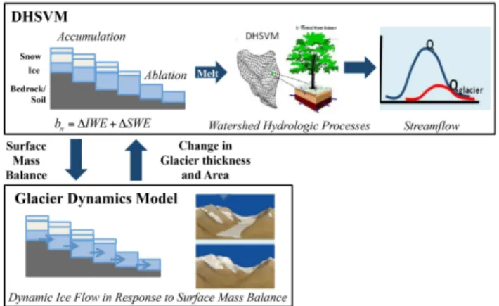
Fig. 1. Schematic of major processes and integration of the Glacier Dynamics Model (GDM) and DHSVM. Accumulation and ablation of snow/ice is simulated in DHSVM. The surface mass balance is calculated and supplied to the GDM at a monthly time-step. Dy-namic ice flow is simulated in GDM based on surface elevation changes. After each monthly glacier dynamics calculation the ice layer in the DHSVM model is updated based on simulated ice flow.
∂S/∂t= ∇xy· D∇xyS+ρice/ρwbn. We solve this equation numerically using a semi-implicit finite-difference scheme that is similar in spirit to the standard Crank–Nicolson method (e.g., Press et al., 2007) but which can optionally ex-ploit the possibility of being “super-implicit” in order to en-sure stability when time steps are large (Hindmarsh, 2001). The essence of our modeling approach is a standard one in glaciology and has been used for simulating the dynamics of ice sheets and ice caps (e.g., Huybrechts, 1992; Marshall et al., 2000; Hindmarsh and Payne, 1996) and of mountain glaciers (e.g., Le Meur and Vincent, 2003; Plummer and Phillips, 2003; Kessler et al., 2006).
In regions of extreme topography, conventional SIA ice-flow models can yield negative ice thicknesses, unphysical behavior that leads to violations of the mass conservation principle upon which Eq. (3) is based. This problem can be addressed by introducing flux limiters when the momen-tum diffusivity Eq. (4) is calculated (Jarosch et al., 2013). Our scheme exploits flux limiters by upwinding ice thick-nessH in Eq. (4), whereas the scheme proposed by Jarosch et al. (2013) applies upwinding to bothH and∇xyS and is somewhat more robust than ours; however, it requires unac-ceptably small time steps to maintain stability. In all other respects the two approaches are comparable.
2.3 Model integration
In order to account for the glacier melt contribution to streamflow from changes in glacier area or volume, the GDM was fully merged into the DHSVM modeling framework as shown in Fig. 1. To predict the present-day ice thickness dis-tribution, the GDM requires subglacial topography and net annual mass balance. On average, snow accumulates in areas
where the net annual mass balance is positive (i.e., above the equilibrium line). As snow accumulates at higher elevations, the GDM transports the ice mass down slope to the areas where the mass balance is negative. By running the model for a long enough spin-up period, the ablation area eventually expands so that annual volumes of accumulated and ablated mass are equal and a steady state is reached.
In the integrated model, we modified the DHSVM surface energy balance snow model to estimate glacier mass balance using sub-daily forcing data. Specifically, the two-layer full energy and mass balance snow model was modified to add an ice layer in order to account for glacier ice melt (Fig. 1). To define total ice volume for the ice layer in the integrated model, the ice layer was initialized with the ice thickness es-timated at the end of the glacier model spin-up time period. As shown in Fig. 1, for each glacier cell the upper two snow layers overlie a bottom layer of glacier ice. When the snow has completely melted, the ice layer becomes exposed and continues to thin by melting at a rate determined using the energy balance approach incorporated in DHSVM. The ice water equivalent (IWE) (m w.e.) of the ice layer is therefore updated at sub-daily time steps only through ice melt and snow densification to ice.
The net monthly glacier mass balance is determined from the change in storage states of SWE and IWE during each month as follows:
bn=1IWE+1SWE, (5)
where1IWE (m w.e.) is the monthly change in the ice layer as a result of ice melt and snow densification and 1SWE (m w.e.) is the monthly change in SWE through snow accu-mulation, melt, and densification to ice in a given month. While the glacier mass balance is tracked by summing changes in snow and ice masses, only changes in IWE (bn,ice)
are supplied as surface mass balance to force the GDM. This avoids instability of the GDM at the sub-annual time steps where a deep ephemeral snowpack overlies lower elevations of the glacier and areas outside of the glacier footprint.
The ice dynamics are computed at a monthly time step in the integrated model. During the glacier model run, the surface topography is updated as a function of net monthly mass balance,bn,ice, and the ice flux in and out of the grid
cell. The ice thickness is updated as a result of changes in the glacier surface topography as follows:
h(i, j, t+dt )=
0, S(i, j, t )≤B(i, j, t )
S(i, j, t )−B(i, j, t ), S(i, j, t ) > B(i, j, t ),(6)
whereS(i, j, t )is the surface elevation (m a.s.l.),B(i, j, t )is the bed elevation (m a.s.l.) at the ith and jth grid cell, and dt
is the monthly time step in years. In the GDM,his the total thickness of the ice layer.
At the end of the each one-month time step of the GDM, the thickness of the IWE layer in DHSVM is adjusted as re-sult of glacier movement as follows:
IWEt(i, j, t+dt )=(S(i, j, t )−(S(i, j, t−dt ) +bn,ice(i, j, t )×
ρice ρw
(7) where IWEt is the amount of ice flux in or out of grid cell,S(i, j, t )is the surface elevation at the current step and
S(i, j, t−dt )is the surface elevation at the previous time step of the GDM.
3 Integrated model implementation: a case study of upper Bow River basin
3.1 Study site description and data
The Bow River originates in the Canadian Rocky Mountains and is a major tributary to the South Saskatchewan River, which flows eastward across southern Alberta (Fig. 2). The upper Bow River has a drainage area of 422 km2above the Lake Louise town site with elevations ranging from 1200 to 3300 m. The mean annual precipitation at the Lake Louise weather station is about 600 mm but is thought to be as high as 1200 mm at higher elevations, mostly in the form of snow. Mean summer (June–August) and winter (December– March) air temperatures are 7◦C and−12◦C, respectively.
Fig. 2. Location of the upper Bow River basin, stream gauging tion above Lake Louise, snow course and Lake Louise climate sta-tion locasta-tions. Glacier cover is based on the Landsat image acquired on 26 August 1986.
The hydrological regime of the upper Bow River is strongly influenced by glacier melt and snowmelt with maximum monthly discharge in summer (June–August) and minimum monthly discharge in February and March.
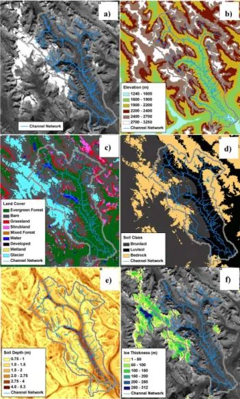
Fig. 3. Input raster data sets used in the study: (a) DEM-derived stream network; (b) 90 meter SRTM DEM; (c) Land cover classes; (d) soil classes; (e) Spatial distribution of DEM-derived soil depth; (f) subglacial topography.
landscape is unknown; hence, its specification in the model is effectively a calibrated parameter. In this application, we ad-justed the soil depths based on the local slope (thinner where steeper), upstream source area (thinner on ridges than in de-pressions), and elevation.
The meteorological forcing data required by the coupled model are precipitation, temperature, wind speed, downward short and long-wave radiation, and relative humidity. In the glacierized portion of the basin, determining these variables is difficult due to various controlling factors such as the oro-graphic influence on precipitation, shadowing effects, and to-pographic aspect variations. In DHSVM, the data records at specific meteorological stations are distributed to each grid cell in the model through interpolation schemes using tem-perature and precipitation elevation lapse rates, or through
gridded temperature and precipitation maps (Wigmosta et al., 1994). Shortwave radiation is adjusted at each grid cell for topographic influences based on month, time of day, and the surrounding topography (solar geometry). Daily data such as minimum and maximum temperature, wind speed and pre-cipitation are available at the Lake Louise station (Eleva-tion: 1524 m) for the time period 1915–2007 (Fig. 2). Due to significant spatial and temporal variability in precipitation and missing records within the station precipitation data, we used 1 km downscaled North American Regional Reanalysis (NARR) daily precipitation data for the 1979–2007 time pe-riod (for a detailed description of the downscaling methodol-ogy, see Jarosch et al., 2012). To run the model at a 3-hourly time step, the daily 1 km NARR precipitation data extracted at the location of the Lake Louise station were temporally disaggregated by equally apportioning days to 3-hourly in-tervals. Temperature, downward short and long-wave radi-ation data were derived at 3-hourly intervals from the daily temperature range and daily total precipitation using methods described in Nijssen et al. (2001). We selected 1979–2007 as our period of analysis.
Daily streamflow data from the gauge station located near Lake Louise were used to evaluate the model results. The Lake Louise gauge station, which is operated by Water Sur-vey of Canada (WSC), was established in 1910 and continu-ous flow data are available until 1986. From 1987 on, stream discharge was only measured for the high flow months (May to October). In addition to measured streamflow data, SWE data from snow course measurements were also available for the model simulation time periods for two different locations within the basin (Fig. 2).
The glacier component of the coupled model requires sub-glacial topography. Bed topography was estimated using the DEM, mass balance fields, thinning rates, and a bed stress model following the methodology described in Clarke et al. (2012) (Fig. 3f).
3.2 Model initialization
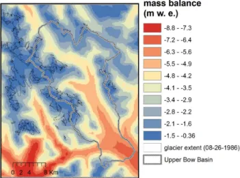
Fig. 4. Spatial distribution of average net mass balance (m yr−1) es-timated using 1 km downscaled NARR precipitation and tempera-ture data for the time period 1979–2008 based on temperatempera-ture index model with 3.9 mm d−1◦C−1degree day factor (DDF).
NARR daily precipitation data and 200 m downscaled NARR temperature data for the period 1979–2007. We used a DDF of 3.9 mm d−1◦C−1 based on Radi´c and Hock (2011) for Peyto glacier located in the study domain (Fig. 2). The an-nual snow accumulation was calculated from the sum of daily solid precipitation assuming that precipitation fell as snow if daily average air temperature was below 0◦C. Using the DDF of 3.9 mm d−1◦C−1, negative mass balance distribution of most glaciers was predicted which is generally consistent with the observed current glacier retreat in this region but may not be representative of the climate condition that al-lows for glacier growth (Fig. 4). We therefore tested a range of increases relative to the computed 1979–2008 average net annual mass balance until the best agreement between ob-served and predicted (1) glacier outlines and (2) fractional glacier cover of the domain was achieved.
Figure 5 shows examples of modeled glacier growth for the Bow River basin with no change in mass balance out-side the glacier boundary but with increases in mass balance for glacierized areas within the basin ranging from 1.3 m to 1.7 m (Fig. 5a–d). Comparing the simulated glacier extents at the end of model spin-up time period (1000 years) with ob-served glacier outlines shows that an increase of 1.6 m above the 1979–2007 average mass balance within the glacierized portion of the basin reproduces the overall extent and ter-minus positions for many glaciers with reasonable accuracy (Fig. 5c). At the end of the glacier model spin-up period, the simulated percent glacier covered area for the study domain is about 9 %, whereas the total percent glacier cover from the 1986 Landsat image is 12 %. The 3 % underestimation of glacier cover is due in part to the use of the 1979–2008 av-eraged net mass balance which reflects the condition of cur-rent negative mass balance. Our sensitivity analysis shows
Fig. 5. Steady-state ice thickness distributions corresponding to in-creases (m w.e. yr−1)applied to averaged 1979–2008 net mass bal-ance shown in Fig. 4. The numbers indicate the increases applied to averaged mass balance only within glacierized areas. Glacier cover extents were delineated from the Landsat image acquired 26 Au-gust 1986.
that an increase of 1.7 m in the mass balance of glacierized areas produces a good match for the glaciers with the most pronounced retreat, but leads to advances for other glaciers (Fig. 5d). Using the 1979–2007 mass balance distribution, augmented by 1.6 m within glacierized areas, as a constant forcing, requires about 650 years for the glacier to reach a steady state.
After the spin-up run was completed, the steady-state glacier geometry derived from the glacier flow model was used as the ice thickness distribution to initialize the inte-grated model. In the inteinte-grated model, glacier ice dynamics are computed at a monthly time interval where the glacier mass balance (net of accumulation and melt of ice) is cal-culated at sub-daily time steps. As described in Sect. 2.3, the ice thickness distribution and glacier extent at the end of each month are updated using Eqs. (6) and (7).
3.3 Integrated model calibration and validation
each of these hydroclimatic variables arguably decreases un-certainty in the glacier melt and streamflow prediction as we desire accurate simulation of multiple first order processes that influence runoff.
The model performance in predicting streamflow was also evaluated using the Nash–Sutcliffe efficiency (NS) (Nash and Sutcliffe, 1970) as
NS=1− P
[Qs(i)−Qo(i)]2
P
[Qo(i)−Qo]2
, (8)
whereQsis the simulated discharge at month or dayi,Qois
the observed discharge andQois the mean ofQo. The case of
NS = 1 represents perfect agreement between simulated and observed discharge, while a NS value less than 0 signifies that the mean is a better estimate than the model estimated discharge.
Because of the distributed nature of both the glacier and DHSVM models, the coupled glacio-hydrologic model is computationally intensive. Additionally, the physical nature of the model limits the number of parameters that can be used for calibration. Key calibration parameters were there-fore identified using one-at-a-time sensitivity analyses and were selected based on first principles. The sensitivity analy-ses were used to determine parameters and constrain param-eter ranges for a multi-objective paramparam-eter search optimiza-tion calibraoptimiza-tion technique (MOCOM-UA, Yapo et al., 1998). Parameters influencing accumulation and ablation of snow and ice: maximum snow albedo, glacier albedo, temperature and precipitation lapse rates, and the soil parameters lateral conductivity and exponential decrease in transmissivity were calibrated. We used this procedure to identify multiple Pareto optimal parameter sets through the optimization of NS, NS of the natural log of daily flows, and error in cumulative glacier mass balance. We used observations of mean annual specific mass balance for the Peyto glacier over the period of 1980– 2007 (Demuth et al., 2009; WGMS, 2009) to compare with our model-predicted glacier mass balance. Area average spe-cific mass balance in the model is computed as follows:
Pn i=1bi Pn
i=1Ni
, (9)
wherebi are mass balance values andNi are the number of grid cells(i=1. . .n) within the glacier extent of study do-main and for individual glaciers (Bow, Peyto). The mass bal-ance values were calculated using Eq. (5).
4 Results
4.1 Calibration and validation of integrated model
Model performance in simulating streamflow was assessed by comparing simulated with observed daily streamflow for both calibration (1981–1986) and validation (1987–2007) time periods. Time series of simulated and observed daily
Fig. 6. (a–f) Simulated (gray) and observed (dashed black) melt season discharge and model bias for WY 1981–1986. The range of uncertainty from parameter selection is indicated by thickness of the plotted simulated and bias lines. (g) Simulated (gray, solid) and observed (circles) monthly mean streamflow for the entire period of analysis (1980–2007).
mean streamflow and bias during the melt season are pre-sented for individual years for the calibration period (Fig. 6a– f), while simulated and observed monthly mean streamflow are presented for the entire period of analysis (WY 1981– 2007) (Fig. 6g). The range of predictions of the five opti-mal parameter sets with equal Pareto ranking are shown for the calibration period, demonstrating uncertainty introduced by model parameter selection. The ranges of parameters for these five optimal configurations are shown in Table 1. For the evaluation period and long-term simulations the parame-ter configuration of these five sets that best captured glacier mass balance was used. The daily and monthly NSE val-ues for calibration years ranged from 0.78–0.81 and 0.91– 0.93, respectively, while for the validation years, the daily and monthly NSE values were 0.77 and 0.87, respectively (Table 2). It should be noted that after 1987, observations are only available during the melt season (May–September), hence the model evaluation mostly reflects model perfor-mance during this time of year, which tends to be more vari-able than the months that were not observed. This tended to result in lower NSE values for the evaluation relative to the calibration period. The calibrated model generally repro-duced the observed hydrographs well, but overestimated the peak summer flow in most years (Fig. 6). On average, the model overestimated the July flow by 13 % and underesti-mated the August and September flow by 2 %.
Table 1. Calibrated DHSVM parameters.
Parameter Analyzed range Optimal range Final calibration
Lateral conductivity 1.0×10⁻⁶–0.01 6.7×10⁻⁴–1.9×10⁻³ 0.00198
Exp. decrease 0.5–3 0.61–1.56 1.37
Precipitation lapse rate (m m−1) 1.0×10⁻⁶–0.001 6.9×10⁻⁵–3.0×10⁻⁴ 0.0002 Temperature lapse rate (C m−1) −0.009–0.0 −0.0087–−0.0079 −0.0087
Maximum snow albedo 0.8–0.9 0.84–0.89 0.85
Glacier Albedo 0.3–0.45 0.30–0.35 0.35
Fig. 7. Mean monthly discharge simulated (gray), observed (black dotted), simulated discharge from glacier melt (black), and glacier contribution (red) during the calibration period (1981–1986). The ranges of the simulated data encompass the predictions of five equally ranked optimal parameter sets, indicating uncertainty from parameter selection.
Table 2. Monthly and daily Nash–Sutcliffe efficiency values for simulated streamflow.
Time period N.S.E Monthly N.S.E Daily
Calibration (1980–1987)∗ 0.91–0.93 0.78–0.81
Validation (1988–2007) 0.87 0.77
Entire period (1980–2007) 0.86 0.76
∗The NSE is calculated from using five optimal parameter sets with equal Pareto ranking.
(August), 3.5 (0.8) m3s−1, as shown in Fig. 7. The combined uncertainty in glacier melt and total streamflow translates to an uncertainty in relative percent glacier contribution of 4 % in August.
To further explore uncertainty in the streamflow predic-tions introduced by the accuracy of the model-predicted glacier cover, a simulation using prescribed glacier ex-tents from satellite estimates (updated at the date of each Landsat scene) was performed and compared with modeled streamflow using the integrated glacio-hydrological model. Running the model with prescribed glacier extents only marginally improved the simulation of streamflow when
Jan Feb Mar Apr May Jun Jul Aug Sep Oct Nov Dec 0
10 20 30 40 (a)
1981 1983 1985 1987 1989 1991 1993 1995 1997 1999 2001 2003 2005 20070 10
20 30 40
(b)
Discharge (m
3/ sec)
Dynamic Static Prescribed Observed
Fig. 8. Observed and predicted (a) mean annual daily (1997–2010), and (b) mean August discharge from model simulations using GDM, static ice and prescribed extent model configurations.
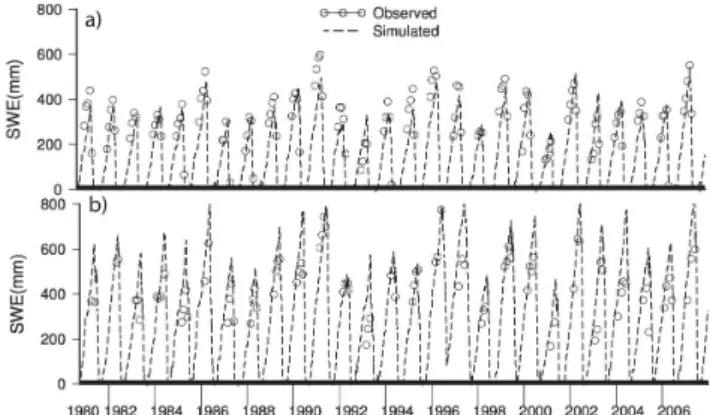
Fig. 9. Measured and model-predicted SWE for two locations in the upper Bow River basin; (a) Bow Summit (2080 m a.s.l.) and (b) Katherine Lake (2380 m a.s.l.).
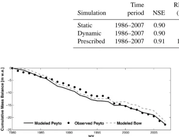
Table 3. Model performance statistics for prediction of monthly mean streamflow for different model configurations.
Time RMSE Jul. Aug. Sept.
Simulation period NSE (cms) bias (%) bias (%) bias (%)
Static 1986–2007 0.90 93.4 13 −5 −4
Dynamic 1986–2007 0.90 92.8 13 −2 −2
Prescribed 1986–2007 0.91 101.4 16 −2 0
Fig. 10. Comparison of predicted cumulative glacier mass balance with observed measurements on Peyto glacier for the period of 1981–2007. Modeled cumulative mass balance for Bow glacier is also shown for comparison.
To test the model performance in predicting the spa-tial variability of snow accumulation, snow course data within the Bow River basin were compared with the sim-ulated SWE, after calibration, for the period of 1980–2007 (Fig. 9). Snow course measurements are conducted several times during the year at two locations (Fig. 2): Bow Sum-mit (2080 m a.s.l.) and Katherine Lake (2380 m a.s.l.). The measurements are reported for the month in which they were conducted but the actual day of observation is unknown. The snow course data at the lower elevation Bow Summit site were accurately reproduced by the model (Fig. 9a), but the model overestimated the maximum SWE at the Kather-ine Lake site in some years (Fig. 9b). The ratio of sim-ulated mean May SWE to observed mean May SWE is 0.94 and 1.18 for the Bow Summit and Katherine Lake sites, respectively.
The modeled cumulative specific mass balance for Peyto and Bow glaciers are shown in Fig. 10, which compare well with the observed cumulative mass balance observed for Peyto glacier for the same period. The missing values of measured mass balance for 1990 and 1991 for Peyto glacier were filled in using the mean annual mass balance value over the entire period for the calculation of cumulative mass bal-ance. By running the model for 1981–2007, we obtained mean annual mass balance of−812 mm w.e. for the Peyto glacier which agreed well with the observed mass balance of −846 mm w.e. averaged over the same period.
Fig. 11. Comparison of monthly model-predicted ice cover extent with Landsat-derived ice cover for years when the cloud-free im-ages were available at the end of melting season for the study do-main. The dates of acquisition of Landsat images are given in Ta-ble A1.
4.2 Role of glacier dynamics on ice cover changes and streamflow response
Comparisons of the predicted ice cover at the end of the melt season each year with the Landsat-derived ice cover are shown in Fig. 11. As discussed in Sect. 3.2, underesti-mation of glacier extent by the GDM at the end of the spin-up time period is evident near the beginning of the simula-tion, but the modeled glacier area compares well with the ob-served glacier area in recent years. To assess the importance of including glacier dynamics in the integrated model, sim-ulations were conducted treating the ice cover as static, (no dynamic ice flow is considered and ice mass is finite). Fig-ure 11 demonstrates the role of glacier dynamics in the accu-rate simulation of glacier extent in time. Neglecting the flow of ice from higher elevations leads to a decline in glacier area that is greater than observed. The implications of this with respect to the simulation of streamflow, is evidenced in late summer flow (Fig. 10b) with relatively larger August model bias of−5 % for simulations with static ice when compared to model bias of−2 % when glacier dynamics are included (Table 3).
a)
b)
c)
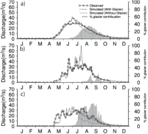
Fig. 12. Comparison of simulated mean annual daily discharge with and without glacier model configurations along with glacier melt contribution in the upper Bow River basin for (a) 1981–2007, (b) cold year (1999) and (c) warm year (1998). The daily observed streamflow data were only recorded from May–October since 1987.
with the highest contribution (30 %) occurring in late Au-gust (Fig. 12a). Figure 12 also compares simulated stream-flow with and without the presence of glaciers and the rela-tive contribution of glacier melt for the warmest (1998) and coldest (1999) years. The warmest and coldest years were se-lected based on the maximum and minimum number of pos-itive degree days, respectively, during the simulation period. In the coldest year (1999), the glacier melt started later in July and the highest contribution to annual flow occurred in late August (15 %) (Fig. 12b). For the warmest year (1998), the glacier melt started early in June with more than 40 % contribution throughout late summer (July–September), and in August glaciers provided up to 47 % of the discharge (Fig. 12c).
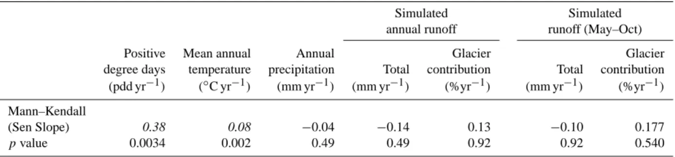
Trend analysis was performed using the Mann–Kendall test (Mann, 1945; Kendall and Gibbons, 1962) and Sen’s slope estimator (Sen, 1968). The Mann–Kendall test is a non-parametric test for monotonic trends that assumes indepen-dent, identically distributed data (Hirsch and Slack, 1984; Helsel and Hirsch, 1988). The Sen’s slope estimator cal-culates the slope using the median of all pairwise slopes in the data set. This analysis showed decreasing trends in both simulated summer (−0.10 mmy r−1) and total annual
(−0.14 mm yr−1)streamflow for the period 1981–2007
(Ta-ble 4); the trends however are not statistically significant. Similarly, statistically significant trends were not identified in annual and summer glacier melt, but both exhibit consis-tent upward trend direction over the simulation period. The downward trend direction in streamflow might be attributable to a decreasing trend in annual precipitation (not statistically significant,pvalue of 0.49) and/or a∼15 % decrease in sim-ulated glacier cover. On one hand, the increasing trend
direc-tion in glacier melt contribudirec-tion to total runoff might be asso-ciated with statistically significant upward trends in positive degree days of 0.38 pdd yr−1 and mean annual temperature
(0.08◦C yr−1). However, these trends may have little impact on annual and summer streamflow in a watershed of this size relative to changes in precipitation and evapotranspiration.
5 Discussion
Simulations from the coupled glacio-hydrological model demonstrate that the representation of the influences of dy-namic processes of glacier accumulation, ablation, and ice flow, in a distributed hydrology model, improves the pre-diction of streamflow response with increasing length of simulation. Running the model with prescribed glacier ex-tents reproduced a similar hydrograph as simulated with the glacier dynamic model, with both configurations predict-ing late summer discharge consistent with the observations (Fig. 8b). The model run with prescribed extents is useful for diagnosing and describing model behavior; however, a major motivation of this study is to progress away from this reliance on external sources of information that may not be available for future prediction (satellite) and may not be directly con-nected to accumulation and ablation processes (independent model predictions) simulated in the hydrologic model.
The calibrated model performed well when compared to the observed hydrographs for most years but it overestimates the peak summer flow in some years which resulted in over-estimation of mean annual daily discharge (Fig. 12b). This overestimation is likely linked to the selection of the pre-cipitation lapse rate, which does not vary in time or space. This lapse rate optimized the simulation of glacier mass bal-ance for Peyto glacier (located north of the drainage area), a primary objective, however, contributed to overestimation of SWE in some years at the higher elevation snow course observation location (Fig. 9b). Additionally, the simple con-figuration of the ice layer, neglecting the representation of englacial and subglacial storage and routing of melt water, may lead to accelerated transport of water on and through glacier masses resulting in enhanced discharge peaks (Jans-son et al., 2003). Future model development efforts should focus on an improved representation of englacial and sub-glacial routing of melt water to improve streamflow predic-tion at finer timescales in highly glacierized watersheds. Fur-ther attenuation of peak flows may also occur as streamflow is routed through several large lakes in the watershed (Fig. 2). DHSVM does not currently account for storage and routing of water in lakes which may also be contributing to the bias in the model predictions of seasonal peak runoff.
Table 4. Trend statistics and trend slopes computed with the Sen’s slope estimator for the time period 1980–2007. Slopes of statistically significant trends are in italic.
Simulated Simulated
annual runoff runoff (May–Oct)
Positive Mean annual Annual Glacier Glacier
degree days temperature precipitation Total contribution Total contribution (pdd yr−1) (◦C yr−1) (mm yr−1) (mm yr−1) (%yr−1) (mm yr−1) (%yr−1)
Mann–Kendall
(Sen Slope) 0.38 0.08 −0.04 −0.14 0.13 −0.10 0.177
pvalue 0.0034 0.002 0.49 0.49 0.92 0.92 0.540
scale of the model (200 m×200 m grid cell). Stream dis-charge observations are calculated using measured stage and a stage–discharge relationship which may be less accurate for individual peak flows. Estimates of glacier extent can be influenced by persistent snow cover from anomalously wet/cold winters or atmospheric moisture (only dry years and days of cloud-free conditions were used in the selection of Landsat scenes, reducing this uncertainty to some extent, Appendix A). Quantifying the uncertainties in the measure-ment of these variables was not included in the scope of this work; however, they could play a role in the performance of the calibrated model.
Additionally sources of errors for simulating streamflow in partially glacierized basins include errors in estimating ini-tial ice thickness distribution which are associated with un-certainty in the mass balance and bed topography (Clarke et al., 2012). A comparison of the distribution of ice after the spin-up period using the estimated bed topography and the surface digital elevation model (SRTM) as the bed topogra-phy reveals a difference of less than 0.05 % in extent and 11 % in ice volume. Based on this comparison, we argue that because the ice volume and ice areas are fairly comparable, the hydrologic response is not likely to differ substantially. This is based on the assumption that using surface topogra-phy (SRTM) as subglacial topogratopogra-phy is likely much worse than any inaccurate estimate of bed topography. Moreover, since there are insufficient data to validate the subglacial bed topography, we assumed that it is correct and only applied adjustments to the mass balance fields that forced the glacier model to grow glaciers in the glacierized parts of the study domain. The adjustment (Sect. 3.2) was made by increas-ing the mean annual mass balance in the glacierized areas to realistically reproduce the shapes and terminus position of the glaciers under the modern climate condition. This ap-proach results in transitions to larger negative mass balance outside of the historical glacier outlines, leading to potential error in estimated ice thickness at these boundaries. How-ever, evidence of this error is not immediately apparent in the simulations of glacier extent over the historical time pe-riod. In this regard, the glacier outlines derived from the 1986 Landsat image were the only indicator of how well the model
reproduced the current glacier shapes and ice thickness dis-tribution. The terminus positions of small glaciers, however, were not reproduced very well, causing a small underesti-mation in the simulated glacier cover at the end of glacier model spin-up run. We found it more important to initialize the ice masses with a mechanistically consistent state using the glacier dynamic spin-up method rather than to match the historical extent with exact precision. Despite the increases in the spatial distribution of mean annual mass, the underes-timation by the model of glacier cover might be attributed to the bias in the NARR data reported by other studies for the Canadian Rockies region (Jarosch et al., 2012). Another im-portant source of uncertainty in estimating the initial glacier mass balance information for the glacier model is the as-sumed value for the DDF, taken as 3.9 mm d−1◦C−1in our study. This estimate that is based on other studies for Peyto glacier (Radi´c and Hock, 2011) may not be representative of the glaciers in the Bow River headwaters.
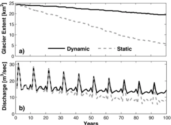
Fig. 13. Hypothetical long-term simulation demonstrating the dif-ferences of simulated (a) glacier extent within the drainage area (422 km2) and (b) August discharge using the dynamic (black, solid) and static (gray, dashed) model configurations. The models were forced with meteorological data from 1998–2007 that was re-peated and perturbed with a linear warming trend (0.03◦C yr−1), creating a 100 years time series.
period are not intended to be an accurate representation of the climate of the next 100 years but rather are for demonstration purposes only.
In Fig. 13, the model configuration that used a static rep-resentation (glacier ice in each glacierized grid cell has finite mass; extent is not fixed) and the configuration that includes the representation of dynamic ice flow (lateral cell to cell movement of ice in response to accumulation and ablation) had much larger deviations between model configurations than were apparent using forcings during the period of his-torical observations (Fig. 8). This is evidenced, for instance, in the simulation of August streamflow shown in Fig. 13 over the course of the 100 years simulation. Without the represen-tation of glacier dynamics, ice accumulating at higher ele-vations does not flow downslope, which in the real system partially replenishes ice melt losses in ablation areas, leading to more rapid glacier recession (Fig. 13a) and declining late summer streamflow (Fig. 13b). The difference between con-figurations in predicted August discharge in the last 10 years of the simulation was more pronounced in low flow years (47 %), where glacier melt has high relative contribution, as contrasted with high flow years (16 %). By the end of the 100 years period August discharge in low flow years using the dynamic and static model configurations was decreased by 19 and 60 %, respectively, as compared with the low flows predicted in the initial decade of the simulation. These results indicate the potential for large over-predictions of reductions in future low flows in model configurations that lack a rep-resentation of dynamic ice flow. Furthermore, the deviation between model configurations was most evident beyond the first 20 years of simulation. While this finding may seem in-tuitive, the results highlight the timescale for which repre-senting glacier dynamics is important. This timescale,
how-ever, is expected to vary with local environmental attributes and climatic forcing.
6 Conclusions
We have documented the integration of a spatially distributed GDM with the distributed hydrology soil–vegetation model (DHSVM) and used the integrated model to investigate the effect of glacier recession on streamflow over the last three decades in the partially glacierized upper Bow River basin, Alberta, Canada. Despite uncertainty in our initial ice thick-ness distribution and glacier extent estimate, the integrated model was better able to capture how climate variations cause changes in glacier cover and streamflow dynamics. Thus, the model more accurately predicts the glacier melt contribution to streamflow when compared with model sim-ulations without glaciers or simsim-ulations that consider ice to be static. Using the integrated model to simulate glacier ef-fects on streamflow variations over the last three decades, we have shown that
1. On average, from 1981–2007, the glacier melt contri-bution to Bow River streamflow is approximately 22 % in summer. This contribution, however, can increase up to 47 % in August for warm and dry years, whereas in cold years, the August glacier melt contribution can be as small as 15 %, and is delayed by about a month. 2. Despite the simulated 15 % decrease in glacier cover
over the period of 1981–2007, no statistically sig-nificant trends were observed in annual and summer runoff. The downward trend direction in summer and total streamflow, however, might be associated with a combined effect of decreases in glacier cover and pre-cipitation.
Table A1. Dates of acquisition of Landsat 5 scenes used in this study.
No Landsat 5 TM
1 28 August 1986 2 27 September 1991
3 2 August 1994
4 7 September 1998 5 15 September 2001 6 13 August 2004 7 16 September 2007 8 12 September 2009 9 26 August 2011
Appendix A
Glacier mapping methodology
The suitability of satellite imagery for estimation of glacier extent depends on cloud cover, the date of acquisition, and the effects of seasonal snow. For this study, we selected (nearly) cloud-free scenes that were acquired late in the dry season (August or September) when seasonal snow was as-sumed to be at a minimum. We used imagery from two sen-sors: Landsat 2 Multispectral Scanner (MSS) and Landsat 5 Thematic Mapper (TM). Although the Landsat satellites have relatively short repeat cycles (ex: 16 days for TM), the pres-ence of cloud cover in mountain environments and the sea-sonal limitation make it difficult to acquire multiple images for any one year.
We selected nine scenes for analysis from the follow-ing years: 1986, 1991, 1994, 1998, 2001, 2004, 2007, 2009 and 2011 (Table A1). All scenes were downloaded from the United States Geological Survey (USGS) Earth Resources Observation and Science (EROS) Center, and were already orthorectified and projected. For all Landsat scenes used in this study, the elevation source for orthorectification was the Global Land Survey (GLS) 2000 data set. All scenes were projected (by EROS) to the North American Datum (NAD) 1983 coordinate system, zone 11N.
We converted Landsat TM digital numbers (DN) to top-of-atmosphere (TOA) radiance using preprocessing tools in ENVI v.4.8. We then converted top-of-atmosphere radiance to surface reflectance using the atmospheric correction model Second Simulation of a Satellite Signal in the Solar Spectrum (6S; http://6s.ltdri.org/) (Vermote et al., 1997). For each cor-rection, we set the target altitude to 2.5 km above sea level, which is approximately the lowest glacier terminus elevation in the basin.
Similar to a previous study in this region (Bolch et al., 2010), we used the ratio of Landsat band 3 to band 5 to map glaciers:
b3/b5=ρVIS
ρNIR
, (A1)
whereρVIS is the reflectance in the visible part of the
elec-tromagnetic spectrum (specifically Band 3 for Landsat TM) andρNIRis the reflectance in the near-infrared portion of the
electromagnetic spectrum (specifically Band 5 for Landsat TM). Paul et al. (2007) found that this method worked well for mapping ice in shadows, although it tends to misclassify water bodies. We created an elevation mask to remove water bodies below 2000 m.
The ratio was computed in ENVI using bands that had been atmospherically corrected. We used GIS to reclassify the resulting calculation into glacier and non-glacier. Next, reclassified rasters were converted to polygons using GIS. Similar to other studies (e.g., Bolch et al., 2010; Racoviteanu et al., 2008), we deleted patches of snow and ice that were smaller than 0.1 km2. Finally, obvious mapping errors, such as lakes above the 2000 m elevation mask, were deleted.
Acknowledgements. This research was supported by NASA grant no. NNX10AP90G to the University of Washington. We thank the five reviewers for their valuable comments and suggestions. The authors are also grateful to Faron Anslow of the Pacific Climate Impacts Consortium (PCIC) for providing Downscaled NARR precipitation and temperature data.
Edited by: M. Weiler
References
Anderson, E. A.: Development and testing of snow pack energy bal-ance equations, Water Resour. Res., 4, 19–37, 1968.
Anderson, E. A.: A point energy and mass balance model of a snow cover, Tech. Rep. 19, NOAA, Silver Spring, Md, 1976. Andreadis, K. M., Storck, P., and Lettenmaier, D. P.: Modeling snow
accumulation and ablation processes in forested environments, Water Resour. Res., 45, W05429, doi:10.1029/2008WR007042, 2009.
Bergström, S.: Development and application of a conceptual runoff model for Scandinavian catchments, SMHI, Report No. RHO 7, Norrköping, 134 pp., 1976.
Bolch, T., Menounos, B., and Wheate, R.: Landsat-based inventory of glaciers in western Canada, 1985–2005, Remote Sens. Envi-ron., 114, 127–137, 2010.
Bowling, L. C. and Lettenmaier, D. P.: The effects of forest roads and harvest on catchment hydrology in a mountainous maritime environment, Water Sci. Appl., 2, 145–164, 2001.
Chennault, J.: Modeling the contributions of glacial meltwater to streamflow in Thunder Creek, North Cascades National Park, Washington, Master Thesis, Western Washington University, USA, 78 pp., 2004.
Clarke, G. K., Anslow, F. S., Jarosch, A. H., Radic, V., Menounos, B., Bolch, T., and Berthier, E.: Ice volume and subglacial topog-raphy for western Canadian glaciers from mass balance fields, thinning rates, and a bed stress model, J. Climate, 26, 4282–4303, doi:10.1175/JCLI-D-12-00513.1, 2012.
Cuffey, K. M. and Paterson, W. S. B.: The physics of glaciers, Aca-demic Press, Amsterdam, 2010.
Demuth, M., Pinard, V., Pietroniro, A., Luckman, B., Hopkinson, C., Dornes, P., and Comeau, L.: Recent and past-century varia-tions in the glacier resources of the Canadian Rocky Mountains: Nelson River system, Terra Glacialis, 11, 27–52, 2008.
Demuth, M., Sekerka, J., and Bertollo, S.: Glacier Mass Balance Observations for Peyto Glacier, Alberta, Canada (updated to 2007), Spatially Referenced Data Set Contribution to the Na-tional Glacier-Climate Observing System, State and Evolution of Canada’s Glaciers, available at: http://pathways.geosemantica. net/, Geological Survey of Canada, Ottawa, 2009.
Dickerson, S. E.: Modeling the effects of climate change fore-casts on streamflow in the Nooksack River basin, Masters thesis, Department of Geology, Western Washington University, USA, 2009.
Fountain, A. G.: Effect of snow and firn hydrology on the physical and chemical characteristics of glacial runoff, Hydrol. Process., 10.4, 509–521, 1996.
Fountain, A. G. and Tangborn, W. V.: The effect of glaciers on streamflow variations, Water Resour. Res., 1, 579–586, doi:10.1029/WR021i004p00579, 1985.
Gardner, A. S., Moholdt, G., Cogley, J. G., Wouters, B., Arendt, A. A., Wahr, J., Berthier, E., Hock, R., Pfeffer, W. T., Kaser, G., Ligtenberg, S. R. M., Bolch, T., Sharp, M. J., Hagen, J. O., van den Broeke, M. R., and Paul, F.: A reconciled estimate of glacier contributions to sea level rise: 2003 to 2009, Science, 340, 852– 857, doi:10.1126/science.1234532, 2013.
Glen, J. W.: The creep of polycrystalline ice, P. Roy. Soc. Lond. A, 228, 519–538, 1955.
Greve, R. and Blatter, H.: Dynamics of ice sheets and glaciers, Springer, Dordrecht, the Netherlands, 77–83, 2009.
Helsel, D. R. and Hirsch, R. M.: Applicability of the t-test for de-tecting trends in water quality variables, edited by: Montgomery, R. H. and Loftis, J. C., J. Am. Water Resour. Assoc., 24, 201– 204, 1988.
Hindmarsh, R. C. A.: Notes on basic glaciological computational methods and algorithms, in: Continuumechanics and Applica-tions in Geophysics and the Environment, edited by: Straughan, B., Greve, R., Ehrentraut, H., and Wang, Y., Springer-Verlag, Berlin, 222–249, 2001.
Hindmarsh, R. C. A. and Payne, A. J.: Time-step limits for stable so-lutions of the ice-sheet equation, Ann. Glaciol., 23, 74–85, 1996. Hirsch, R. M. and Slack, J. R.: A nonparametric trend test for sea-sonal data with serial dependence, Water Resour. Res., 20, 727– 732, 1984.
Hock, R.: Temperature index melt modelling in mountain areas, J. Hydrol., 282, 104–115, 2003.
Huybrechts, P.: The Antarctic ice sheet and environmental change: a three-dimensional modeling study, Ph.D thesis, Vrije Univer-siteit of Brussel, Germany, 1992.
Huss, M., Farinotti, D., Bauder, A., and Funk, M.: Modelling runoff from highly glacierized alpine drainage basins in a changing cli-mate, Hydrol. Process., 22.19, 3888–3902, 2008.
Huss, M., Jouvet, G., Farinotti, D., and Bauder, A.: Future high-mountain hydrology: a new parameterization of glacier retreat, Hydrol. Earth Syst. Sci., 14, 815–829, doi:10.5194/hess-14-815-2010, 2010.
Immerzeel, W., Droogers, P., De Jong, S., and Bierkens, M.: Large-scale monitoring of snow cover and runoff simulation in Hi-malayan river basins using remote sensing, Remote Sens. Env-iron., 113, 40–49, 2009.
Immerzeel, W. W., Van Beek, L. P. H., Konz, M., Shrestha, A. B., and Bierkens, M.: Hydrological response to climate change in a glacierized catchment in the Himalayas, Clim. Chang., 110.3-4, 721–736, 2012.
Jain, S.: Snowmelt Runoff Modeling and Sedimentation Studies in Satluj Basin using Remote Sensing and GIS, Ph.D. thesis, Uni-versity of Roorkee, India, 2001.
Jansson, P., Hock, R., and Schneider, T.: The concept of glacier stor-age: a review, J. Hydrol., 282, 116–129, 2003.
Jarosch, A. H., Anslow, F. S. and Clarke, G. K. C.: High-resolution precipitation and temperature downscaling for glacier models, Clim. Dynam., 38, 391–409, doi:10.1007/s00382-010-0949-1, 2012.
Jarosch, A. H., Schoof, C. G., and Anslow, F. S.: Restoring mass conservation to shallow ice flow models over complex terrain, The Cryosphere, 7, 229–240, doi:10.5194/tc-7-229-2013, 2013. Jost, G., Moore, R. D., Menounos, B., and Wheate, R.:
Quantify-ing the contribution of glacier runoff to streamflow in the up-per Columbia River Basin, Canada, Hydrol. Earth Syst. Sci., 16, 849–860, doi:10.5194/hess-16-849-2012, 2012.
Kendall, M. and Gibbons, J. D.: Rank Correlation Methods, Edward Arnold, A division of Hodder & Stoughton, A Charles Griffin title, London, 29–50, 1990.
Kessler, M. A., Anderson, R. S., and Stock, G. M.: Modeling to-pographic and climatic control of east-west asymmetry in Sierra Nevada glacier length during the Last Glacial Maximum, J. Geo-phys. Res., 111, F02002, doi:10.1029/2005JF000365, 2006. Laramie, R. L. and Schaake, J. D.: Simulation of the continuous
snowmelt process. Ralph M. Parsons Laboratory for Water Re-sources and Hydrodynamics, Massachusetts Institute of Technol-ogy, 1972.
Le Meur, E. and Vincent, C.: A two-dimensional shallow ice-flow model of Glacier de Saint-Sorlin, France, J. Glaciol., 49, 527– 538, 2003.
Lindström, G., Johansson, B., Persson, M., Gardelin, M., and Bergström, S.: Development and test of the distributed HBV-96 hydrological model, J. Hydrol., 201, 272–288, 1997.
MacGregor, K. R., Anderson, R., Anderson, S., and Waddington, E.: Numerical simulations of glacial-valley longitudinal profile evolution, Geology, 28, 1031–1034, 2000.
Mann, H. B.: Nonparametric tests against trend, Econometrica, J. Econom. Soc., 13, 245–259, 1945.
Marshall, S. J., Tarasov, L., Clarke, G. K., and Peltier, W. R.: Glacio-logical reconstruction of the Laurentide Ice Sheet: physical pro-cesses and modelling challenges, Can. J. Earth Sci., 37.5, 769– 793, 2000.
Martinec, J.: New methods in snowmelt-runoff studies in represen-tative basins, in: IAHS Symposium on Hydrological Character-istics of River Basins, IAHS Publ. No. 117, 99–107, 1975. Moore, R., Fleming, S., Menounos, B., Wheate, R., Fountain, A.,
Nash, J. and Sutcliffe, J.: River flow forecasting through conceptual models part I – A discussion of principles, J. Hydrol., 10, 282– 290, 1970.
Nijssen, B., Schnur, R., and Lettenmaier, D. P.: Global retrospective estimation of soil moisture using the variable infiltration capacity land surface model, 1980–93, J. Climate, 14, 1790–1808, 2001. Paul, A., Kääb, A., and Haeberli, W.: Recent glacier changes in the
Alps observed by satellite: Consequences for future monitoring strategies, Global Planet. Change., 56, 111–122, 2007.
Plummer, M. A. and Phillips, F. M.: A 2-D numerical model of snow/ice energy balance and ice flow for paleoclimatic interpre-tation of glacial geomorphic features, Quaternary Sci. Rev., 22, 1389–1406, 2003.
Press, W. H., Teukolsky, S. A., Vetterling, W. T., and Flannery, B. P.: Numerical Recipes, 3rd Edn., The Art of Scientific Computing, Cambridge University Press, 2007.
Racoviteanu, A. E., Williams, M. W., and Barry, R. G.: Optical re-mote sensing of glacier characteristics: a review with focus on the Himalaya, Sensors, 8, 3355–3383, 2008.
Radi´c, V. and Hock, R.: Regionally differentiated contribution of mountain glaciers and ice caps to future sea-level rise, Nat. Geosci., 4, 91–94, 2011.
Rees, H. G. and Collins, D. N.: Regional differences in response of flow in glacier-fed Himalayan rivers to climatic warming, Hy-drol. Process., 20, 2157–2169, 2006.
Schindler, D. and Donahue, W. F.: An impending water crisis in Canada’s western prairie provinces, P. Natl. Acad. Sci. USA, 103, 7210–7216, 2006.
Sen, P. K.: Estimates of the regression coefficient based on Kendall’s tau, J. Am. Stat. Assoc., 63, 1379–1389, 1968. Sicart, J. E., Hock, R., and Six, D.: Glacier melt, air
tem-perature, and energy balance in different climates: The Bo-livian Tropics, the French Alps, and northern Sweden, J. Geophys. Res.: Atmospheres (1984–2012), 113, D24113, doi:10.1029/2008JD010406, 2008.
Singh, P. and Bengtsson, L.: Hydrological sensitivity of a large Hi-malayan basin to climate change, Hydrol. Process., 18, 2363– 2385, 2004.
Stahl, K. and Moore, R.: Influence of watershed glacier coverage on summer streamflow in British Columbia, Canada, Water Resour. Res., 42, 1–5, 2006.
Stahl, K., Moore, R., Shea, J., Hutchinson, D., and Cannon, A.: Coupled modelling of glacier and streamflow response to future climate scenarios, Water Resour. Res., 44, W02422, doi:10.1029/2007WR005956, 2008.
Storck, P.: Trees, Snow and Flooding: an Investigation of Forest Canopy Eff ects on Snow Accumulation and Melt at the Plot and Watershed Scales in the Pacific Northwest, Ph.D. thesis, Univer-sity of Washington, 2000.
Storck, P., Bowling, L., Wetherbee, P., and Lettenmaier, D.: Appli-cation of a GIS – based distributed hydrology model for predic-tion of forest harvest eff ects on peak stream flow in the Pacific Northwest, Hydrol. Process., 12, 889–904, 1998.
Thyer, M., Beckers, J., Spittlehouse, D., Alila, Y., and Win-kler, R.: Diagnosing a distributed hydrologic model for two high-elevation forested catchments based on detailed stand-and basin-scale data, Water Resour. Res., 40, W01103, doi:10.1029/2003WR002414, 2004.
Uhlmann, B, Jordan, F., and Beniston, M.: Modelling runoff in a Swiss glacierized catchment—part I: methodology and applica-tion in the Findelen basin under a long-lasting stable climate, Int. J. Climatol., 33, 1293–1300, doi:10.1002/joc.3501 2012. Vermote, E. F., Tanré, D., Deuze, J. L., Herman, M., and Morcette, J.
J.: Second simulation of the satellite signal in the solar spectrum, 6S: An overview, IEEE Trans. Geosci. Remote Sens., 35, 675– 686, 1997.
Weertman, J.: On the sliding of glaciers, J. Glaciol., 3, 33–38, 1957. Whitaker, A., Alila, Y., Beckers, J., and Toews, D.: Application of the distributed hydrology soil vegetation model to Redfish Creek, British Columbia: model evaluation using internal catch-ment data, Hydrol. Process., 17, 199–224, 2003.
Wigmosta, M. S., Vail, L. W., and Lettenmaier, D. P.: A distributed hydrology-vegetation model for complex terrain, Water Resour. Res., 30, 1665–1680, 1994.
WGMS: Glacier Mass Balance Bulletin No. 10 (2006–2007), edited by: Haeberli, W., Gartner-Roer, I., Hoelzle, M., Paul, F., and Zemp, M., ICSU(WDS)/IUGG(IACS)/UNEP/UNESCO/WMO, World Glacier Monitoring Service, Zurich, 2009.