Using irregularly spaced returns to estimate multi-factor models : application to Brazilian equity data

Using Irregularly Spaced Returns to Estimate Multi-Factor Models:

Application to Brazilian Equity Data

Álvaro Veiga

Departamento de Engenharia Elétrica - PUC Rio Leonardo R. Souza

Graduate School ofEconomics (EPGE) - Fundação Getúlio Vargas

Abstract - Multi-factor models constitute a use fui tool to explain cross-sectional covariance in equities retums. We propose in this paper the use of irregularly spaced returns in the multi-factor model estimation and provide an empirical example with the 389 most liquid equities in the Brazilian Market. The market index shows itself significant to explain equity returns while the US$/Brazilian Real exchange rate and the Brazilian standard interest rate does not. This example shows the usefulness of the estimation method in further using the model to fill in missing values and to provide intervaI forecasts.

Keywords: Multi-Factor ModeI, Missing Data JEL Classification: C32, C53 e G 13

1 -Introduction

Emergent markets frequently suffer from Iow Iiquidity and tend to concentrate most of transactions on a few Iiquid assets. Subramanian (2001, p.77), for example, shares this view for bond markets. As to equity markets, the Brazilian one comprises about 1190 different stocks but almost 40% have not been negotiated in the Iast year and 32% of the remaining has been negotiated Iess than once a month. As a consequence, for many stocks there will be no price for a large proportion of days. There will be still more days for which one cannot compute daily returns, since they require the existence of transactions in two subsequent days.

analysis of risk and return 1• A market model can provi de the expected vaIues of missing

prices and returns. Sharpe (1964) proposed the Capital Asset Pricing Model (CAPM) to explain asset returns. However, a number of papers provided empirical evidence against the CAPM. For example, Bhandari (1988) and Chan, Hamao and Lakonishok (1991). Furthermore Fama and French (1992) and Jegadeesh (1992) show that the market beta has little power in explaining cross-sectional asset returns, meaning that some common "factor" could further explain the retums. Ross (1976) proposed the Arbitrage Pricing Theory (APT), which allowed more than one factor to explain the assets returns and consequently diversify risk premia. However, these factors are non-observable. Reinganum (1981) and Mei (1993) use autoregressive approach to explain the hidden factors. Chen, Roll and Ross (1986) introduced macroeconomic variables to explain stock returns in a multi-factor linear regression. It is common practice in financiaI institutions to use this model to explain assets returns, where the factors are called risk factors.

Then a circular problem may arise: these market models must be estimated before computing the expected value of missing prices and returns, but if the proportion of missing data is high many numerical problems may surge and bias the estimation. A biased estimation will lead to poor price filling. Note that models are usually for returns since they are statistically more attractive than prices, so that it is the number of missing daily returns that matters. In this paper, we propose an estimation method to the multi-factor model which makes use of irregularly spaced returns, enabling the use of every historical price available and thus increasing efficiency. In other words, it permits calculations with percentage of existing daily (c1osing) prices as low as 5% in a year of data, whereas traditional estimation do noto

The multi-factor model can then be used to estimate missing prices and also to estimate the h-step ahead interval forecast for returns, h = 1, 2, 3. The motivation to use up to three steps ahead comes from the fact that the Brazilian Market liquidity system determines that parties involved in a transaction have three days to liquidate it.

To evaluate the estimation method, we ran a back test with 389 stock prices over the period ranging from August 25, 1998 to February 28, 2001. Two main important

aspects of the estimated model, with practical implications to the users of the data were

examined. First, we examine its ability to produce good estimation of missing prices. This was done comparing each observed price to the estimated value that would be

produced by the model if this particular price was missing. Second, the h steps ahead

interval forecasts were evaluated by comparing the nominal and observed frequencies of values in the 5% tails, which is an important measure in risk analysis.

For a comparative evaluation, the same experiment was run to some other

imputation methodologies frequently used by practitioners such as repeating the last price or mimicking the market index return, as well as the same multi-factor model estimated

only with the available daily returns. All these are nested under the same multi-factor class of models. We conclude that the multi-factor model estimated using irregular retums globally outperforms alI the others, including the traditional regular returns

estimation. Furthermore, the Brazilian Equity Market Index show to significantly explain equity retums but the US$ - Brazilian Real exchange rate and the Brazilian inter-bank ovemight interest rate do not.

The next Section presents the notation used further in this paper and the

methodology proposed here, while Section 3 shows an empirical example with Brazilian equity data. Section 4 offers some concluding remarks.

2 - Notation and Methodology

In this Section we describe the notation and the methodology used in this paper.

The price of equity j at time t is denoted by

P/

and the (log-)retum of the same equity at

time t by:

Ri ₁

=

ln[ _pi

ｾｩ＠

)

=

ln(pi) ₁ -ln(pi ) _{l-I ,}

l-I

(1)

where j

=

I, ... , ] (J

=

389 in the experíment) and t

=

1, ... , T. The advantage of using

log-retums instead of simple returns is that the log-retum yielded in 't days ('t integer and

greater than one) is the sum ofthe daily log-retums over the 't-days período

A Multi-Factor model describes a linear relation between the return of equity j

and some market indicators, taking the form

Rl _(fJl)TX j '

1 - 1 1 +c_{1 ,} (2)

where fJ/ is the vector of coefficients of equity j at time t,

Xr

is the vector of market

indicators (possibly log-returns) at time t and c/ errors supposedly iid, c/ - N(O,a2

). l.1

We allow the coefficients to vary slowly and smoothly in time to let the relationship between returns and indicators be dynamic. However, the study of this variation is not in the scope of the paper. To deal with this variation in a simple fashion, we estimate all models within the exponential smoothing (EWMA) framework (l.P. Morgan, 1995), which is briefly explained in Section 2.3. This procedure is common standard in practice within financiaI institutions.

For instance, if the return of a market index and the overnight inter-bank interest rate2 are used as risk factors (or simply factors), as well as a constant, the model becomes thus:

(2A)

where Xl.1 is the market index return and X 2.1 the interest rate at time t. In the notation

of Equation (2), Xl

=

[;1.1

1

Xv

and

Given there is no missing value in the estimation window, the estimation is obtained via weighted least squares, with the weights exponentially decreasing with the age of the data. The missing value of equity j occurs when there is no trade of the equity j

at time (day) t. Its imputation at time t based on this model uses the returns expected values given the current (daily) market indicators at time t. The VaR (Value at Risk, which "measures the worst expected loss over a given time interval under normal market conditions at a given confidence leveI", lorion, 1997, p. xiii) estimation h days ahead, however, requires that the market indexes be forecast.

2.2 - Irregularly Spaced Returns

Emergent markets contain a number of illiquid equities which are not negotiated every day, unlike the market indicators. For these equities, the estimation window is scattered with missing values. Considering the existence of these windows, one must pay

attention to returns which interval is not one day, but say 't days. However, data are available every day. Figure 1 illustrates these non-full estimation windows and the irregular returns.

Figure 1: Estimation window with missing data and irregular returns Equity data

ｌ］ｧｗｾｭｵ］＠

day traded missing value

ｾ＠ '&

\

/

f i I

I

O • • • O O • O • O • • • O • O O

Market indicators data

ｾ＠

f i I

I

•

• • •

•

• • • •

•

• • • • • • •

•

• •

• • • • • • •

•

• • • •

• •

days of trade

Thus, one needs to define the 't-days return at time t for equity j. Let it be:

(3)

Moreover, equalling the right-hand sides of equations (1) and (2) and rearranging yields:

i_ i i T i

lnp' -lnp,_1 +

(P,

)

X, + c, . (4)

Applying Equation (4) to t

=

t, t-l, t-2, ... , t-'t+ 1 and summing up gives:

r-I r-I

In

p,i

=

In ｐＬｾｲ＠ +

L

(P/_i)T X'_I +

L

C/_I·

(5)

Iffor practical purposes

P/

and ｃｔｾＬＱ＠ are considered (almost) constant on the interval [t-., t]3, and since c/ is iid, then, using (3), (5) rewrites as:

r-I

ｒＡＮｾ＠

=

(P!

l

L

X'_i +

W!.r ,

(6)

where

r-I

W/.

r

=

í>L;

W/.

r - ｎＨｏＬｲｃｔｾＮＬＩＮ＠

i=O

2.3 - Exponentially Weighted Moving Average (EWMA)

The EWMA framework is also known as RiskMetrics (J.P. Morgan, 1995) and its motivation is that the dynamics of what is under study (e.g., equity data) changes with time but no assumption is to be made upon these changes besides the change is smooth. So, the older are the data the less weight it must have attached to. These weights decrease

exponentially with time, driven by the smoothing parameter À, O < À < 1. The day t*

return is thus given À times the weight given to the return of t*+ 1. The parameter K, in turn, determines the number of effective days to be used in the estimation window. The mean of equity j returns at time t is then estimated by:

K-I

fi:

=

LÀi

(1-À)R/_i • (7)

The covariances between returns of equities and j at time t, as well as the variance of equity i are estimated by:

(8)

Depending on K, the right-hand sides of Equations (7) and (8) must be multiplied

by a constant C so that the sum ofweights CÀm(l-À) is the unity (C ｾ＠ 1 as K ｾ＠ 00). For the sake of simplicity, the constant C was omitted from Equations (7) and (8). We do not take into account the loss of a degree of freedom in ca1culating the mean. Little effect though there will be in our results since we use K = 252 (corresponding to one year of

data) o It is usual to consider the mean of retums as being zero, simplifying more these equationso However, this assumption is not made hereo An overview on EWMA is given in Alexander (1996)0

2.4 - Methodology

2.4.1 - Estimation with Irregular Returns

Some equities have trading prices for all days in the estimation windowo In these cases, Equation (2) is considered and a weighted least squares procedure, with EWMA

weights, yields the estimates of

P:

for each equity j at the current time to This is done

through the equation:

fi:

=

(XTWX)-I XTWRj , ₍₉₎

where

Rj

=

Rirl

=

[R/_K +1 R/_K +2 000 R/_I R/

r

is the vector of equity j returns;

x

=

X Kx(p+l)

=

=

Xl.t -K+1

X1,t-K+2

for all equities); and W

=

W KxK

=

o

O

case, p market indicators are consideredo

000 Xpot-K+I

000 X p,t-K+2

is the design matrix (the same

Xp.1

O

O O

is the weights matrix4

0 In this

O

The lines of Rj, X and W correspond to one day period (daily returns)o However,

whether there is a missing value in the estimation window, (6) instead of (2) must be

considered, so that all lines corresponding to a same t-days retum Will collapse into one single line in the redefined matrices

W,

X and Wo The redefined matrices are as follows:

4 In fact, if ali the weights in W are multiplied by the same constant, the estimates do not change, as the

change in the inversion ofXTWX compensates the change in XTWRio That is why the weights do not match

Ài

!

o

O

TI

O

À>

W=W_{K K )x )} = _{T 2}

O

O O

lA)

T K)

r,-I

IXU-i,-m m=O

r,-I

ｾｘｉＬｲＭｩＬＭｭ＠

m=O

T1-l

... ""

ｾ＠

x

p.1-il-m m=O

r,-I

... ""

L...,

x

p.l-i2-m m=O

(lO)

where there are Kj+ 1 prices (Kj possibly irregularly spaced returns) available in the

estimation window for equity j; 'tk, k

=

1,2, ... , Kj, is the interval ofthe k-th return in the estimation window; and ik is the time past between the k-th return of equity j and the current time t (in other words, the age of the return, measured in days in the present implementation). So, in addition to account for exponentially decaying weights, W

assigns weights inversely proportional to the variances ofthe errors W:r 5.

2.4.2 - Missing Values Imputation

In the more general case, the imputation of missing values can occur at any point of the estimation window, although the results with real data shown here are only from imputing data at the end of it (current day). For the sake of simplicity, consider

Pr

=

In ｾｪ＠ • Following (5), the expected value of pr, conditional on

/3/,

the vector of

market indicators

X

and the next existing price (forward or backward respectively for equations Il.A and Il.B) is given by:

,,-I

E(Pr / Pr-r,

,/3/

,X)

=

Pr-r, +

(/3/)

TI

X r_i (II.A)

;=0

r,-I

E(p, / P/H,

,/3/

,X) = P/H, -

(/3//

2:

X/H,-i (11.B)

i=O

Using (l1.A) and (11.B), replacing

/3/

by its estimate

P/,

we reach the estimates of a missing price conditional on the next (forward or backward) existing price and the risk factors. The estimates are as follows:

(12.A)

r,-I

P

X+r,

=

Pt+r, -

(P/

/

ｾ＠

X/+r,_i . (12.B)

Thus, if the missing value to be imputed is at the end of the estimation window, (l2.A) is used. If it is in the beginning, (12.B) is used. Otherwise, (12.A) and (12.B) are combined so as to yield minimum variance, using the fact that the errors with j fixed (same equity) are iid as follows:

(13)

For details on the minimum variance estimator see Neter et aI (1996, p.400).

2.4.3 - Estimation of Interval Forecasts

We consider here the interval forecast (lF) estimation as an ad hoc procedure, ignoring uncertainties of many sorts and making some further simplifying assumptions. The exact parametric predictive density given the specified model would require the account of the variance of estimated coefficients, even if the assumptions hold. If one is to consider the problem through the view of the c1earinghouse, which guarantees the transactions, two-sided IF's must be supplied. This is because both parties may default, which means that the c1earinghouse may have to buy or sell the equity in the market three

days after the transaction is agreed. The IF is computed as the following. Let E(Rt+t:.'t) be

the expected value of equity j 't-days retum at time t+t given

/3/

and

X

:

The first simplifying assumption is that the coefficients

13

are independent in

relation to the factors XI. Note that this assumption may not hold since the l3's may be influenced by the factors magnitude. But considering this assumption true, it is straightforward to estimate the expected value of the .-days ahead return given the information until time t by:

Ê(R/H,r

I

t)

=

(jJ/)TÍX/+/

(15)

1=1

To use (15), the risk factors must be forecast. However, the method used to forecast the risk factors is beyond the scope of the paper. Now we must estimate the variance .-days ahead, and to facilitate computations one more assumption is made. The second simplifying assumption is that the risk factors are homoskedastic, or at least that

their variances vary slowly in the t-days ahead period. AItematively to making this assumption, this variance may be viewed as conditional on the current circumstances conceming volatility and risk. As it was assumed before that the coefficients

13

are

(almost) constant and the errors are serially independent, the variance of equity j .-days

return at time t+t may be approximated by:

ｏＢｾＩ＠

,/+r.r ==

ｲｬｏＢｾＮＱ＠

+,8/

'COV(XJ,8/],

(16)

Ignoring the uncertainty caused by the estimation of the coefficients

13,

this

variance can be estimated at time t as:

(17)

L

=

explln(p,) + Ê(R/H .r ) +

rI

(a /2, Kj - p -I)rr RJ.I+r.r

J

and

U

=

explln(p,) + Ê(R/+r.r) +

rI

(1-a / 2, Kj - p -l)rr RJ"I+r.r

J,

(18)

where (l(.,V) is the inverse cumulative distribution function of a Student's t random variable with v degrees of freedom, and Kj is the number of observations available for equity j at the estimation window. The lower bound, if desired, can be calibrated using the semi-variance (see Gastineau e Kristzman, 1996, p. 250, for example) to estimate

VAR(Xi .r ). The semi-variance is the mean of the squared negative deviations from the

mean. The VaR of l-a/2 confidence leveI is given by the lower bound ofthe l-a IF.

3 - Empirical Example with Brazilian Equity Data

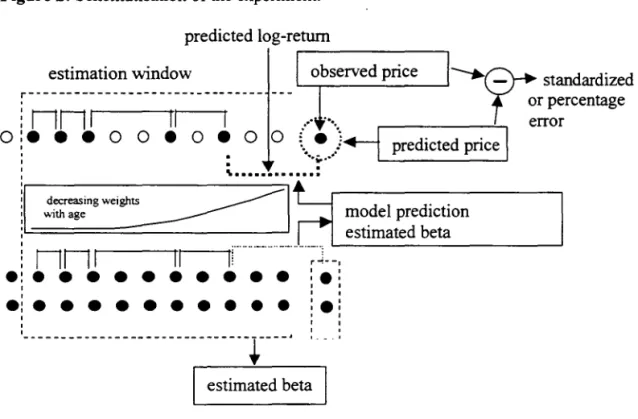
The database consists of389 stock prices (the most liquid in the Brazilian Market) over the period ranging from August 25, 1998 to February 28, 2001. The results are divided in two sections, the first dedicated to the imputation of missing values and the second to the IF estimation. To access the accuracy of the missing values imputation, each single observation in the database within specified pattems is deleted at a time and filled in as is schematised in Figure 2. This enables the computation of error statistics, where the error is the difference between the filled in and the observed data. In tum, the IF is estimated for every observation in the database within the same specified pattems, one two and three steps ahead, and its coverage verified. The specified pattems are: two subsequent prices available; a price available at t and t+2; and a price available at t and t+ 3. These pattems are motivated by the fact that the parties involved have three days to liquidate the transaction, and thus a c1earinghouse must estimate a IF for the equity price up to three days ahead in order to access its risk in the case of default.

3.1 - Missing Values

Exchange Market Index), where the equity is supposed to follow the market return in the

absence of the real price. Note that both methods are nested in the multi-factor (naif.

l3i,t

i

= O, i = O, 1, ... , p ; proxy:

I3k)

= 1, where

I3k,t

i is the coefficient referring to the market index retum, and

l3i)

= O, i

"*

k). A further comparison inc1udes the multi-factor estimated conventionally, that is, on1y with regular (daily) retums. In a companion paper, Souza and Veiga (2001) implemented an E-M algorithm (Dempster, Laird and Rubin, 1977) with principal component analysis to compete against the multi-factor with irregular retums on the same database. Their conc1usion is that the multi-factor outperforms the E-M for the equities with less than 95% of data available.

Figure 2: Schematisation ofthe experimento predicted log-retum

estimation window

r---innl

II

o:. e • o o • o

ＭＭＮｾ＠

standardized

or percentage

I

.. ' ....

....-____ --'...,

error

e o o : ....•...

_{• "io'"} Ｚｾ＠ _{ｾ＠ t predicted price}

I

decreasing weights with age

,

...

:

model prediction estimated beta

...•. _ ...

__

... _ ... '---'

nn r-I ----tlr-I ---tI!

• •

.,

. . .

•

• •

•

•

•

• • •

, ,

' ... ---- -_ .. -_ .. --

--

-_ .. ----

-

--

--.

ＭｾＭＭ

-

_.

r -1--.

:

.:

, , , ,

:.:

, ,

, , , ,

1- . I

estimated beta

To find the best multi-factor configuration, we test three values of the EWMA smoothing constant, A

=

0.98, 0.99 and 1. These high values of A are justified by the size of the estimation window (252 business days, approximately one year of data), which in tum is justified by the inc1usion of many low liquidity equities in the comparison6.

The factors used to explain the equities returns were the Brazilian Market Index

(lBV), based on the most liquid equities negotiated in the São Paulo Stock Market; the Brazilian standard ovemight interest rate (eDI); and the US DollarlBrazilian Real exchange rate (US$). Different combinations of these three factors were compared

against each other. The comparison is done by means ofthe following statistics:

RMSSE: root mean square of standardized errors

(19)

where N is the total number of cases of interest over time and equities and 't is the time

horizon, 't = L 2. 3 .. In order to keep the comparison fair, â RJ ,I.r is estimated by EWMA

and is the same for alI methods. The standardization by a volatility estimate is because

some equities are more volatile than others, and so their prediction errors can be compared without some equities dominating the statistic in spite of others.

DC: direction of change statistic

1 " , · .

DC(r)

=

N L sgn(R,'c)

*

sgn(R,'r)'

1./ {

I, if a >0 where sgn(a)

=

O, if a

=

O

-1, if a < O

(20)

This statistic is related to the proportion of times the predicted retum has the same sign than the actual retum (predict the equity price wilI rise and it indeed rises or predict it wilI falI and it falIs). It measures the difference between the number of times the

method predicts the direction of change correctly and the number oftimes the direction of change is predicted incorrectly, relatively to the total number of cases.

MAPE: mean absolute percentage error

1 (

p;

pJ)

MAPE(r) = -

I

I.r - I . N I.; P/

(21)

While the RMSSE measures the error In the retum prediction, the MAPE

measures the percentage error in imputed prices. The fonner has a more statistical

approach while the latter a more financiaI approach.

Tables 1 and 2 (one day ahead) and Figures 3-5 (three days ahead) show the results for the naif, the proxy and the multi-factor with irregular retums using the

IIIBUOfECA MARIO HENRIQUE SIMONSH

foIlowing factors: no factor - only the constant (Of), the market index retum (IBV), IBV and the one day standard interest rate (lBV & CDI), and the IBV and the retum of the

US$fBrazilian Real exchange rate (IBV & US$). Ali the multi-factor results refer to À

=

0.99. The results referring to the remaining values ofÀ, 0.98 and 1, are not ｳｨｯｾ＠ as they

are in general worse than those with À

=

0.99. The results are grouped by the adjusted R2

(ofIBV) as it was the feature that most explained the difference between methods.

Table 1: RMSSE one day ahead by adjusted R2.

adj. R2 na"if ｾｲｯｸｹ＠ Df IBV IBV & COI IBV & US$ # cases

-20% - O 1,03 1,12 1,04 1,03 1,05 1,05 6339

0-5% 0,96 1,01 0,97 0,95 0,96 0,96 23839

5 -15% 0,94 0,96 0,94 0,90 0,91 0,91 31151

15 - 30% 0,93 0,88 0,93 0,84 0,84 0,85 24975

30 -45% 0,87 0,77 0,88 0,73 0,74 0,74 13053

45 - 55% 0,89 0,71 0,90 0,67 0,68 0,71 5339

55 -65% 0,81 0,63 0,82 0,61 0,62 0,63 3332

65 -75% 0,79 0,55 0,80 0,54 0,55 0,55 1679

75 - 85% 0,77 0,47 0,79 0,46 0,47 0,48 1070

85 - 90% 0,83 0,42 0,86 0,39 0,39 0,39 440

90 - 95% 0,77 0,30 0,77 0,29 0,29 0,29 343

95 - 100% 0,73 0,19 0,77 0,20 0,21 0,20 141

ali 0,88 0,85 0,90 0,81 0,83 0,84 111701

Table 2: MAPE one day ahead by adjusted R2•

adj. R2 na"if ｾｲｯｸｹ＠ Of IBV IBV & COIIBV & US$ -20% - O 0,048 0,054 0,050 0,051 0,054 0,052

Figure 3: RMSSE three days ahead by adjusted R2.

1.20

-ｾＺｅﾷ＠

•.•

_{ｾﾷＮｾｾｾｾ＠}

0.20 0.00

Figure 4: MAPE three days ahead by adjusted R2•

0.140

-+-naif -proxy

Of

---r-.--IBV --.-IBV & COI -+-IBV & US$

O 0.120 100

ｾ＠

-+- naif

ｧＺｧｾｧ＠

_::

ｾ＠

__

ＭＭＭＭＭ［ｾＭＭＭＺＺ［ｾｾｾ＠

-proxy

0.040

ｾＮＮＬＮ＠

. - - ' - . - . =t

--o

Df

0.020 ---

ｾＮＮＮ＠

_'_, IBV

0.000

-Figure 5: De three days ahead by adjusted R2•

1.00

0.80

-0.60 ---,.,....-::. 0.40

0.20

0.00 _____!IIIF"----"

.

ＧＮｾｾ＠

. .

.

.

ｾｉｂｖＦｃｏｉ＠

-IBV & US$

-+-naif -proxy

Df

-r--IBV

ｾｉｂｖＦｃｏｉ＠

The RMSSE and the MAPE show that overall the multi-factor with irregular returns using only the market index returns performs best. This means that in general the market index is signiticant to explain equity returns, whereas the US$/Brazilian Real exchange rate and the Brazilian inter-bank overnight interest rate are not so. However, the reader must keep in mind that 50 of these equities form the index, so that the experiment is biased in favour of this index (each of the two assets with most weight make up around 10% ofthe index, while the following tive make up between 4% and 6% each\ On the other hand, the majority of these equities have a negligible weight in the indexo

The nalf outperforms the multi-factor by slight margin where the adjusted R2 _is

low, and so does the proxy where the R2 _{is high. However, as the R}2 _{begins to rise the}

nalf tends to be outperformed by all others, and furtherrnore the proxy is the worst method for low R2 (which is within the expected since the R2 is related to the explication coefficient for the IBV only, and the proxy uses the IBV with j3 = 1). The Direction of Change statistic points to the proxy (the market index return) as the best indicator for the rise or fall of each equity price three days ahead. The results for one, two (not shown) and three days ahead are qualitatively similar.

3.1.1 - Irregular Versus Regular Returns

In this Section, the irregular returns multi-factor model is compared with the conventional factor with daily returns. The simple fact that the conventional multi-factor needs two subsequent days of trade to provide a daily retum compares favourably to the multi-factor with irregular returns. It is because the regular returns multi-factor discards the information of single prices (with no negotiation ofthe equity in the previous or in the next day) and part ofthe information brought by a price in the end of a block of prices, whilst the irregular returns version uses all prices. For this reason, there can be equities whose coefficients j3 can be estimated by the irregular retums version but not conventionally. There are cases where no daily return can be computed in one year, but a

number ofirregular ones are available8. As long as there are degrees offreedom enough

to reasonably estimate the coefficients

13,

the irregular returns multi-factor can be used, and in the present paper we considered 10 retums (less than 4% of data available, considering a 252 days estimation window) as a lower bound to estimate the regression. Table 3 compares the number of cases in the database for which there were enough data so that each version could estimate the coefficients

13.

Note that the regular retums enable

the estimation onIy one third of the times the irregular retums do when there are at most 5% of data (prices) available, and approximately half ofthe times when there are between 5% and 15% of data available. From 65% of data available on both enable the same number of estimations in the database. The comparison reported below takes into account onIy the cases where both versions were able to estimate the coefficients. Since we stipulated 10 returns as a minimum to estimate the regression, the case where between 0% and 5% of the prices are available is restricted to 1 I or 12 prices existing in the 252 days estimation window. In view of this, 33 cases out of 100 where I 1 or 12 prices were available and 10 daily returns could be computed seem toa many, as one would expected existing prices scattered randomly over the estimation window. However, there are many cases in the database where a liquid equity started being negotiated during the period under study, having less than 13 prices in one year past because it was less than 13 days old then.

Table 3: frequency of estimation windows with more than 10 retums available (with an existing price in the end), for regular and irregular retums multi-factor. The cases are grouped by percentage of existing prices within the window.

0- 5% 5 - 15%15 - 30%30 - 45%45 - 55%55 - 65%65 - 75% 75 - 85%85 - 90%90 - 95%95 - 100% 100%

regular 33 824 3628 6073 5027 5976 7049 10260 7262 9131 24248 30822 irregular 100 1446 4006 6278 5097 6003 7049 10260 7262 9131 24248 30822

Figures 6 - 9 show the RMSSE and the MAPE for filled in data 1 and 3 days ahead. Note that the results are now grouped by percentage of existing prices in the estimation window, unlike the comparison with the nalf and the proxy. The irregular

retums version yields almost always better results. The greatest difference appears when there are between 5% and 55% of prices available for imputation I day ahead9 _and

between 0% and 75% of prices available for imputation 3 days ahead. When the horizon increases to 3 days ahead, the advantage of the irregular returns version over the conventional one becomes more apparent. When alI the prices are available, both versions are equal by definition and consequently their results are so. This also means that their results approximate more the more data exist in the estimation window.

Figure 6: RMSSE of filled in data from regular and irregular retums multi-factor, 1 day ahead, grouped by percentage of existing prices in the estimation window.

1.25 1.20 ＭＭＭＭＺＰＭＮｾＭＭ 1.15-1.10 - -ＭＭＭＮｦＭＭＭＭＭｾ｣｟｟ＺＺｾＮＭＭＭＭＭＭＭＭＭＭＭＭＭ

1.05 1 " " " ' = ,

-1.00

--0.95 - ＭＫＭＭｾＭＭＭＭＭＭＭＭＮＭＭ ____

-0.90 - ＭＫＭＭＭＭＭＭＭＭＭＭＭＭ］Ｍ］ｾｉＡＺＺ］ｾＭＭ 0.85 --0.80 ＭＭｾＭＭＭＭＭＭＭＭＭＭＭＭＭ

ｾｲ･ｧｵｬ｡ｲ＠

_irregular

It is clear by these results that the multi-factor with irregular retums outperforms the conventional multi-factor, in addition to enable the estimation in cases where the conventional cannot be applied. As pointed out before, as the proportion of existing data approaches the unity, both estimation methods (with only regular and with irregular retums) are more similar and hence have more similar results.

Figure 7: MAPE of filled in data from regular and irregular retums multi-factor, 1 day ahead, grouped by percentage of existing prices in the estimation window.

0.060 -

---0.050 ＭｾＭＭＭ -

-0040 --- --- - . , =

-0:030 __ __ _______

ｈ｟ｾＭＭＭ］］ｴｉ｟ｾＭｾＭ

___

0.020

0.010 0.000

--+-regular _irregular

Figure 8: RMSSE of filled in data from regular and irregular returns multi-factor, 3 days ahead, grouped by percentage of existing prices in the estimation window.

1.15 -

----1.05 ＭＭＭＭＭＭ］ＴｾＭｾ＠ ...

-1.00 0.95

0.90

0_85 -0.80

---+-regular --- irregular

0.110 ｾＭＭＭＭＭＭＭＭＭ ｾＭＭＭＭＭＭＭＭＭ

0.100 ＭＭＭＫｾＭＭＭＭＭＭＭＭＭＭＭＭＭＭＭＭ

0.090 - ' \ 0

-0.080 ｾＭｉＭＭＭＭｐｾ＠ ＭＧ＾ＮＬＮＭＭＭＭＭｾＭ

-0.070

0.060 - - _______ ＢＧＬＮＮＮＭＢＧｾ］］ＭｉｾＭＭＭＭＭ

0.050

-0.040

3.2 - IF estimation

-regular -irregular

-Clearly the irregular multi-factor outperforms the nayf in filling in missing values, especially for higher values of the adjusted R2• The proxy is slightly outperformed,

especially for lower values of that statistic. From the previous results, we chose the best configuration to be the one that uses only the IBV as a factor. The 90% two-sided IF estimates (obtained via equation (18» from this configuration are tested in this Section, together with a benchmark. The benchmark is the use of plain EWMA

O ..

= 0.99) to estimate the IF of the equity price, under the normal assumption. The IF estimates from equation (18), however, need estimates for the risk factors volatilities. A volatility proxy using the highest and the lowest prices (assuming the log-price is a Brownian Motion) is tried (denoted by "irreg MF u-d" in the Tables 4 and 5), as well as the squared returns

(denoted by "irreg MF"). Both were computed using EWMA weights and À = 0.90 (other values were tried and yielded no better results). The volatility proxy using the highest and lowest prices is taken from Parkinson (1976) and is given by:

ｾ＠ 2 (u - d)2

a

=-.::...-....:...-41n2 ' (22)

closing prices are found in Gannan and Klass (1980). All volatility proxies in the experiment use only data up to t-l to estimate the volatility at time t. We also tried the semi-variance but the results were no better and are not sho\\11.

The percentage of cases the price fell below (above) the 90% central IF is sho\\11 in Tables 4 and 5, grouped by adjusted R2

• The starred numbers are significantly (u

=

0.05) different from the nominal percentage of 5%. The significance was obtained using approximate 95% confidence intervals based on the DeMoivre-Laplace Central Limit Theorem. More powerful tools to check coverage of IF's are given in Christoffersen (1998), but we felt them unnecessary for the present analysis.

Table 4: Percentage of cases below or above the 90% one day ahead central IF grouped by adjusted R2

•

Below 90% IF Above 90% IF

Adj. R2 irreg MF irreg MF u-d EWMA irreg MF irreg MF u-d EWMA # cases -20% - 0% 0,042* 0,042* 0,044* 0,065* 0,065* 0,063* 5540

0-5% 0,037* 0,036* 0,039* 0,058* 0,057* 0,056* 24339 5 -15% 0,033* 0,032* 0,037* 0,056* 0,056* 0,052 31820 15 - 30% 0,034* 0,036* 0,033* 0,055* 0,058* 0,053* 26063 30 -45% 0,033* 0,038* 0,030* 0,047 0,053 0,044* 12705 45 - 55% 0,037* 0,044* 0,034* 0,051 0,059* 0,047 5058

55 -65% 0,030* 0,041 0,023* 0,044 0,053 0,041* 2922

65 -75% 0,034* 0,044 0,026* 0,040 0,053 0,037* 1611

75 - 85% 0,038 0,056 0,025* 0,037 0,053 0,033* 885

85 - 90% 0,051* 0,071* 0,033* 0,054 0,063 0,036 336

90 - 95% 0,027 0,043 0,013* 0,040 0,064 0,030 299

95 -100% 0,035 0,052 0,026 0,044 0,096* 0,043 115

Table 5: Percentage of cases below or above the 90% three days ahead central IF grouped by adjusted R2

•

Below90% IF Above 90% IF

Adj. R2 irreg MF irreg MF u-d EWMA irreg MF irreg MF u-d EWMA # cases -20% - 0% 0,016* 0,016* 0,017* 0,045 0,045 0,045 5312

0-5% 0,017* 0,017* 0,018* 0,046* 0,046* 0,045* 23492 5 -15% 0,021* 0,021* 0,023* 0,053* 0,053* 0,051 31150 15 - 30% 0,034* 0,037* 0,029* 0,059* 0,063* . 0,056* 25799 30 - 45% 0,035* 0,040* 0,029* 0,057* 0,065* 0,052 12609 45 - 55% 0,049 0,062* 0,036* 0,069* 0,081* 0,062* 5041 55 - 65% 0,045 0,055 0,025* 0,052 0,062* 0,047 2900 65 - 75% 0,051 0,069* 0,025* 0,062* 0,079* 0,049 1602 75 - 85% 0,066 0,090* 0,030* 0,052 0,069* 0,041 878 85 - 90% 0,087* 0,110* 0,054 0,084* 0,107* 0,066 335

90 - 95% 0,050 0,070 0,027 0,060 0,084* 0,030 299

Tables 4 and 5 show that the multi-factor model estimated with irregular returns brings an improvement to the plain EWMA in the central IF estimation, the exception being the upper bound three days ahead. The EWMA is a benchmark used in many financiaI institutions and showed to be conservative on the present data. In general, the methods tend to be more conservative in the IF lower bound than in the upper bound, which means that an asymmetric predictive distribution could do better. However, using the semi-variance approach did not yield any better resulto

As to the market index volatility proxy for the multi-factor, using the squared retums (irreg MF) performs better than using highs and lows (irreg MF u-d) for three days ahead, while the inverse occurs for one day ahead. As the irreg MF u-d seems to be too liberal for three days ahead, yielding an excessive number of cases above and below the IF when the adjusted R2 is above 45%, we recommend using the squared returns (weighted by EWMA) to estimate the factor volatility in the irregular returns multi-factor.

4 - Conclusion

In this paper we proposed the use of retums which are not regularly spaced in time to estimate the multi-factor model for equity returns. The multi-factor model is a simple but efficient tool to explain cross-sectional covariance in equities retums. The model showed itself useful to estimate missing data as well as to provi de interval forecasts for future retums. Furthermore, the use of irregular retums enables the estimation in cases where using only regular (daily) returns would not.

Acknowledgements

This work was carried out in 2001 when both authors were working as consultants to

AIgorithmics Brazil and through AIgorithmics Brazil to the Sao Paulo Exchange Market (BOVESPA) and its c1earinghouse (CBLC). The second author (Souza) greatly

acknowledges the financiaI support received afterwards by F APERJ, which enabled to wrÍte the academic version ofthe paper.

References

Alexander, C.

o.

(1996), "Evaluating RiskMetrics as a risk measurement tool for your operation: what are its advantages and limitations?", Derivatives: Use, Trading and Regulalion, 2, 3,277-284.

Alexander, C. O. and Leigh, C.T. (1997), "On the covariance matrices used in

Value-at-Risk models", Journal of Derivatives, 4, 3, 50-62.

Bhandari, L. C. (1988), "DebtlEquity ratio and expected common stock retums: empirical evidence", Journal of Finance, 43, 507-528.

Chan, L., Hamao, Y. and Lakonishok, J. (1991), "FundamentaIs and stock retums in

Japan", Journal of Finance, 46, 1739-1764.

Chen, N-F, Roll, R. and Ross, S.A (1986), "Economic forces and the stock market",

Journal of Business, 59, 3, 383-403

Christoffersen, P.F. (1998), "Evaluating Interval Forecasts", International Economic Review, 39, 4,841-862.

Dempster, AP., Laird, N. M. e D.B.Rubin (1977). "Maximum likelihood from

incomplete data via the EM algorithm", Journal oflhe Royal Statistical Society B, 39,

pp.I-38.

Fama, E. and French, K. (1992), "The cross-section of expected stock retums", Journal ofFinance, 47, 427-466.

Garman, M.B. and Klass, M.J. (1980), "On the estimation of security price volatilities

from historical data", Journal of Business, 53, 1,67-78.

Jegadeesh, N. (1992), "Evidence of predictable behavior of security returns", Journal of Finance, 45,881-898.

Jorion, P. (1997), Value at Risk: a new benchmark for controlling market risk, Irwin Professional Publishing, Chicago.

J P Morgan (1995), RiskMetrics - Technical Document, 3rd edition, Morgan Guaranty Trust Company, New York.

Mei, J. (1993), "Explaining the cross-section retums via a multi-factor APT model", The

Journal of Financiai and Quantitative Analysis, 28, 3,331-345.

Neter, J., Kutner, M.H., Nachtsheim, C. and Wasserman, W. (1996), Applied Linear Regression Models, Irwin.

Parkinson, M. (1980), "The extreme value method for estimating the variance of the rate ofretum", Journal of Business, 53, 61-65.

Reinganun, M. R. (1981), "Empirical tests of multi-factor pricing model. The Arbitrage Pricing Theory: some empirical results", Journal of Finance, 36,2,313-321.

Ross, S. (1976). "The arbitrage theory of capital asset pricing", Journal of Economic Theory, 13, 341-360.

Sharpe, W.F. (1964), "Capital Asset Prices: a theory of the market equilibrium under conditions of risk", Journal of Finance, 19, 425-442.

Souza, L. and Veiga. A. (2001), "A comparison between the EM and the irregular returns multi-factor for missing data in emergent stock markets", AIgorithmics Brazil internaI report.

ＧｬＹｾ＠

v ,

j\(

ｾＢｾａｃￂｏ＠

GETULIO

ｖａｒｇｾ＠

-f.-BIBLIOTECA

MARIO

H!NiHOUE

It ....

SJIiI

I

ｕｾ＠

-312023'

UJü2 -

ISP!/'2Q)

2-［ｾｦｬｶｺｨｫＭ

000312023

FUNDAÇÃO GETULIO VARGAS

BIBLIOTECA

ESTE VOLUME DEVE SER DEVOLVIDO A BIBLIOTECA NA ULTIMA DATA MARCADA

N.Cham. PIEPGE SA S729u Autor: Souza, Leonardo

Título: Using irregularly spaced retums to estimate multi-f

ＱＱＱｉＱＱＱＱｾＱｬ＠

Ｂｾｉ＠

11"1 011111111

［ＺＲｾｾＲＳ＠